A bounded-degree network formation game
Abstract
Motivated by applications in peer-to-peer and overlay networks we define and study the Bounded Degree Network Formation (BDNF) game. In an -BDNF game, we are given nodes, a bound on the out-degree of each node, and a weight for each ordered pair representing the traffic rate from node to node . Each node uses up to directed links to connect to other nodes with an objective to minimize its average distance, using weights , to all other destinations. We study the existence of pure Nash equilibria for -BDNF games. We show that if the weights are arbitrary, then a pure Nash wiring may not exist. Furthermore, it is NP-hard to determine whether a pure Nash wiring exists for a given -BDNF instance. A major focus of this paper is on uniform -BDNF games, in which all weights are 1. We describe how to construct a pure Nash equilibrium wiring given any and , and establish that in all pure Nash wirings the cost of individual nodes cannot differ by more than a factor of nearly 2, whereas the diameter cannot exceed . We also analyze best-response walks on the configuration space defined by the uniform game, and show that starting from any initial configuration, strong connectivity is reached within rounds. Convergence to a pure Nash equilibrium, however, is not guaranteed. We present simulation results that suggest that loop-free best-response walks always exist, but may not be polynomially bounded. We also study a special family of regular wirings, the class of Abelian Cayley graphs, in which all nodes imitate the same wiring pattern, and show that if is sufficiently large no such regular wiring can be a pure Nash equilibrium.
1 Introduction
In this paper, we define and study a graph-theoretic game, called the Bounded Degree Network Formation (BDNF) game. An -BDNF game models the distributed formation of a directed network with nodes in which each node selfishly selects out-going links, with the goal of minimizing a cost that is a function of its distances to other nodes in the network. We focus on the following cost function: For each ordered pair of nodes, we have a weight that captures the traffic rate from to , and we define the cost of a node as the total weighted distance to all the other nodes. In this setting, we call a network or a wiring stable if no node can improve its cost by an unilateral rewiring. In other words, a stable wiring represents a pure Nash equilibrium of the BDNF game.
Bounded-degree network formation games arise in the context of popular applications like unstructured peer-to-peer (P2P) file-sharing [14, 6] and overlay routing [3] when the participating nodes behave strategically and select first-hop neighbors in order to selfishly optimize their own utility. In both applications, bounded degrees are in place — albeit for different reasons. In unstructured P2P file-sharing, nodes employ scoped-flooding or multiple parallel random walks to reach other nodes and thus have to adhere to small out-degrees in order to protect the network from getting clogged with queries. Overlay routing systems have been proposed for allowing nodes to route their traffic through alternative overlay paths that offer better resilience or quality of service than the standard ones offered by the native IP routing mechanism. Such systems run full fledged link-state routing protocols at the overlay layer and thus have to monitor and disseminate link-state information for all the overlay links. Initial systems, like RON [3], assumed a full-mesh overlay topology and as a consequence did not scale well (could go up to around 50 nodes). Subsequent proposals [19, 13] have achieved better scalability by putting constraints on the out-degree of nodes so as to reduce the number of overlay links that need to be monitored.
The second defining characteristic of our network formation game – the directionality of links – is also well-reflected in several applications from both families. In P2P file-sharing, link directionality is usually explicitly specified in the protocols used for implementing the system, whereas in routing, it arises as a consequence of the employed business strategies [5]. Considering the aspect of routing (for queries or traffic), we note that our choice of the cost function for the BDNF game implicitly assumes that shortest-path routing is in place. This is indeed the case in overlay routing systems, where the nodes have global awareness of the overlay topology by participating in the link-state overlay routing protocol, and thus can execute a shortest-path algorithm and determine such routes. In P2P file-sharing systems that employ scoped flooding or random walks, routing can deviate from being shortest-path. We notice, however, that it can be made approximately close to being shortest-path by increasing the scope of flooding or the density of parallel random walks (at an extreme case, full flooding guarantees that a destination will be reached through a shortest-path).
1.1 Our Results
In this paper, we study the structural and complexity-theoretic properties of stable wirings. We first consider general non-uniform games, in which the weights are arbitrary.
- •
For any , and any sufficiently large, there exists a collection of weights for which the -BDNF game has no pure Nash equilibrium. Furthermore, it is NP-hard to determine whether a pure Nash wiring exists for a given -BDNF instance with arbitrary weights. These results are in Section 3.
The main focus of this paper is on uniform games, where all the weights are 1.
- •
One of our main results is a proof that every uniform -BDNF game has a pure Nash equilibrium wiring. Our proof is constructive and our stable wiring enjoys the property that the radius of each node is at most , implying that the total distance is at most twice as much as the best possible network that could be constructed by a central network designer. This result appears in Section 4.2
- •
Although the complete characterization of stable wirings for uniform -BDNF games remains an open research problem, we establish some general properties of all stable wirings. We show that every stable wiring for a uniform -uniform game is almost fair: the cost of any node is within times the cost of any other node. We also explore the possibility of completely fair stable wirings by studying regular wiring patterns formed by Abelian Cayley graphs, a special class of vertex-transitive graphs. We show that for any , no Abelian Cayley graph with degree and nodes is a pure Nash equilibrium for for some constant . These results appear in Section 4.3.
Our final set of results, which appear in Section 5, concern best-response walks on the configuration space defined by uniform games.
- •
We show that starting from any initial configuration, strong connectivity is reached within steps. Convergence to a pure Nash equilibrium, however, is not guaranteed. We present simulation results that suggest that loop-free best-response walks always exist, but may not be polynomially bounded.
Our experiments have suggested several interesting open questions and conjectures, which we present in Section 6.
1.2 Related Work
Our model for network formation is inspired in large part by [9] where they defined and studied a similar network creation game. Rather than assuming a fixed budget of outgoing links as in our network formation game the authors in [9] consider undirected links, and the nodes optimize a cost which is the sum of the number of edges, scaled by a parameter , and the sum of distances to the rest of the nodes. They present several results on the price of anarchy, which is the ratio of the cost of the worst-case Nash equilibrium to the social optimum cost [11]. Further results on this network formation are obtained in [1]. In [16] a variant of this game is studied, in which the nodes are embedded in a metric space and the distance component of the cost is replaced by the stretch with respect to the metric. They obtain tight bounds on the price of anarchy and show that the problem of deciding the existence of pure Nash equilibria is NP-hard. Network formation under the requirement for bilateral consent for building links is studied in [8]. [12] presents an experimental study of network formation games involving non-unit link lengths.
Network formation games have also been studied in the context of Internet inter-domain routing. A coalitional game-theoretic problem modeling of BGP is introduced in [18] and studied further in [15]. Also related is the work on designing strategy-proof mechanisms for BGP [10] as well as the recent work on strategic network formation through AS-level contracts [5].
2 Preliminaries and Problem Definitions
Consider a set of nodes . Each node is equipped with: (1) a link-budget , specifying the maximum number of nodes to which can establish outgoing directed links (or wires), and (2) weights , indicating ’s preference for communicating messages to (for convenience ). Node establishes a wiring by connecting each one of its links to a different node. A global wiring is taken from the superposition of the individual wirings of all the nodes, defining essentially an edge-set of a graph with vertex set . The cost for node under a global wiring is taken by a weighted (by preference) summation of its distances to all destinations, i.e., , where denotes the length of a shortest directed path from to over the global wiring ( if such a directed path does not exist).
Definition 1.
(BDNF game) The Bounded Degree Network Formation game is defined by the tuple , where:
- •
is a set of players, which in this case amount to the nodes of a graph.
- •
is the set of strategies available to the individual players. is the set of strategies available to . Strategies correspond to wirings. A game in which each player can select any one of the possible wirings is called symmetric. An asymmetric game is one in which node is allowed to select nodes from a subset , and therefore may have fewer than strategies.
- •
is the set of cost functions for the individual players. The cost of player under an outcome , which in this case is a global wiring, is .
We say that a wiring is stable if it is a pure Nash equilibrium for the BDNF game. In the rest of the paper we focus on BDNF games with the following two characteristics. (1) All direct links have unit weight11 1 Such a distance model implies that the end-to-end delay owes to relaying at the intermediate nodes and not due to the crossing of the actual links. Such is the case when the relay nodes are rather slow whereas the links themselves are fast, which is a plausible model for P2P file-sharing and overlay routing applications that run on software over non-specialized hardware. In [12], the authors have studied experimentally the case of non-uniform link weights using synthetic and actual measurement data. and therefore the distance becomes equal to the number of hops on a shortest path from to over . In [12] it is shown that in this case, the best-response of node can be obtained from the solution of a -median problem on an asymmetric distance function obtained from flipping the distance function of the residual wiring . (2) All nodes have the same link budget . We call such games -uniform when all the weights are the same (e.g., all equal to 1) and -non-uniform, otherwise.
3 Nonuniform Games
In this section we ask whether pure Nash equilibria exist for all instances of the non-uniform game. We start with asymmetric non-uniform games, in which a node is allowed to select neighbors from a subset of , with this subset being different for different nodes in the general case. We show that pure Nash equilibria may not exist in this case. Then we argue that given an asymmetric non-uniform game with no pure Nash equilibria, we can construct an equivalent symmetric non-uniform game, thereby establishing that symmetric non-uniform games may not have pure Nash equilibria as well.
Lemma 1.
There exist instances of the asymmetric -non-uniform game, for all and such that they have no pure Nash equilibria.
Proof.
It is sufficient to prove the desired claim for -non-uniform games since for or , the result follows from the -non-uniform case by just forcing all of remaining wirings to link to specific nodes, using appropriate weights.
The basic idea is to construct an instance of an asymmetric -non-uniform BDNF game that encodes the pay-off structure of a “matching pennies” game [17]. To construct such an instance we define an object that we call the “Gadget” (see Fig. 1 for an illustration). Our Gadget is made out of two sub-gadgets, sub-gadget0 and sub-gadget1. Sub-gadget0 consists of five nodes: a central one (0C), two bottom ones (left, 0LB and right, 0RB), and two top ones (left, 0LT and right, 0RT). Similarly for subgadget1.

The solid lines in Fig. 1 are used for originating nodes that can connect only to a single other node. Such is the case for the two top nodes of each sub-gadget that can connect only to a specific bottom node of the other sub-gadget. Node 0LT can connect only to node 1RB, node 0RT only to node 1LB, and similarly for the other sub-gadget.
The dashed links in the same figure represent choices the originating node can make. The central node of a sub-gadget can connect to only one of the top nodes of the same sub-gadget. So for example 0C can connect its single outgoing link to either 0LT or to 0RT. Each one of the two bottom nodes of a sub-gadget can connect to either the central node of the same sub-gadget or to another node not depicted in the figure.
Having defined the players and the asymmetric strategy sets we move on to define the weights . The central node in each sub-gadget is only interested in reaching the central node of the other sub-gadget, i.e., 0C wishes to reach 1C and vice versa, neither one, however, is allowed to establish a direct link to the other, and therefore they have to go first through a top node of the same sub-gadget and then through a bottom node of the other sub-gadget. The bottom nodes are primarily interested in reaching the cross-over top node in the same sub-gadget, i.e., 0LB is interested in reaching 0RT. Now, if a bottom node cannot reach its corresponding cross over top node, then it prefers to connect to the node that is not shown in the figure. The top nodes only care to reach the unique node they are allowed to connect in the other sub-gadget.
We claim that this gadget has no pure Nash equilibria. Let 0C be connected to say 0LT and let 1C be connected to 1RT. Then it is clear how the bottom nodes will connect: 0RB will connect to 0C, 0LB will connect to the not depicted node, 1LB will connect to 1C, and 1RB will connect to the not depicted node. But now 1C can reach 0C while 0C cannot reach 1C. Hence 0C is unstable and has to switch from 0LT to 0RT, which gives it a path for reaching 1C. This has the following immediate effects on the bottom nodes of sub-gadget0: 0LB switches to connecting to 0C and 0RB switches to connecting to the not depicted node. This, however, breaks 1C’s path to 0C, causing it to switch to 1LT. Now, the bottom nodes of sub-gadget1 switch accordingly, thereby breaking 0C’s path to 1C and causing it to switch back to its initial connection to 0LT. The bottom nodes of sub-gadget0 return to their initial positions, thereby breaking 1C’s path to 0C, and causing it to switch back to its original connection to 1RT. This causes the bottom nodes of sub-gadget1 to return to their initial positions. At this point the gadget has return to its initial configuration. Thus it is easy to see that like puppies chasing their tails the two sub-gadgets will be continually switching. Hence there is no pure Nash equilibrium. ∎
Lemma 2.
There exist instances of the symmetric -non-uniform game with and such that they have no pure Nash equilibria.
Proof.
As in the case of Lemma 1, it is sufficient to prove the desired claim for -non-uniform games. We will construct an instance of a symmetric -non-uniform game in which, although the nodes are allowed to select neighbors from the entire node set , in a pure Nash equilibrium they would have to connect to neighbors belonging to the same subsets as with the asymmetric -non-uniform game of Lemma 1. We will implement this property using the weights . In this spirit, the solid line that connects a node from the top of a sub-gadget to a fixed node at the bottom of the other sub-gadget (as shown in Fig. 1) can easily be implemented by setting and zeroing out the weights to all other nodes. Similarly, the “switch” from the central node of a sub-gadget to the two top nodes of the same sub-gadget can be implemented by setting: (1) , (2) , with , where indicates the central node of the other gadget, and (3) zeroing out the weights to all other nodes.
Implementing the switch from a bottom node to either the central node of the same sub-gadget, or to another node (not depicted in Fig. 1) is a little more involved. Let’s set , , and , where denotes ’s cross-over node at the top of the same sub-gadget. If denotes the disconnection cost we need to enforce that:
The first inequality guarantees that a bottom node will never establish a direct link to its cross-over node at the top of the same sub-gadget. The second one guarantees that if the link from the central node to the cross-over does not exist, then the bottom node will connect to the not depicted node. The last inequality guarantees that if the link from the central node to the cross-over node exists, the bottom node will connect to the central node. The three inequalities can be jointly satisfied by picking positives : , and setting: and . We have now showed that there exists an instance of symmetric non-uniform game that if it had a pure Nash equilibrium, the asymmetric non-uniform instance of Lemma 1 would also have one. Since the last lemma establishes that such a pure Nash does not exist, it follows that there exist symmetric non-uniform games with no pure Nash equilibria. ∎
Theorem 1.
Given a non-uniform instance of the game (symmetric or asymmetric) it is NP-complete to determine whether the instance has a pure Nash equilibrium.
Proof.
Proof sketch: The proof is by reduction from 3SAT with variables and clauses. The basic idea is to model each variable as a sub-gadget (represented as a circle in Figure 2) with the state where C is pointed to LT representing the variable is set to 1 and C is pointed to RT representing that the variable is set to 0. Variables are indifferent between their two states. Each clause is represented by a vertex that can pick one of its 3 literals to connect to. A literal in a clause is represented by a connection, through an intermediate vertex, that is made to the corresponding variable’s sub-gadget if and only if the sub-gadget is oriented in the right way, i.e., to guarantee that the variable is satisfied. There is a base node that connects to all the clauses. Finally we have a gadget whose central nodes are interested in connecting to the base node if and only if all the clauses connect to their intermediate nodes, i.e., the can all be satisfied.

The weights are set up so that if the formula is satisfiable then each of the variable gadgets have an appropriate orientation and there would be a pure Nash equilibrium. If the formula is not satisfiable then the gadget would continually toggle. ∎
4 Uniform Games
We counterbalance the result in Section 3 by showing that stable graphs do exist for uniform games. In particular, we show that for every integer and any , the uniform -BDNF game has a stable graph. In fact, there may be multiple stable graphs. We first present our constructed graph and then prove its stability. We next present in Section 4.3 some structural properties of stable graphs and argue that certain natural regular wirings, in which all nodes imitate the same wiring pattern, are not stable.
4.1 Description of our constructed stable graph
Granted and , let denote the maximum depth of a full -nary tree with nodes. Let denote the number of remaining nodes, the number of complete -tuples that can be formed based on , and the resulting untupled nodes. We construct the following graph:
The tree: We use nodes to construct , a full -nary tree with levels. Nodes are labelled according to the in-order traversal of , with node 1 being the root.
The additional roots: We consider the remaining nodes as additional roots (conceptually) placed next to node 1 and connected to the same set of children (nodes , which we call the hubs).
The bridge: We call the rightmost leaf of the bridge. We connect of the bridge’s links to corresponding untupled roots and the remaining ones to corresponding heaviest hubs. The weight of a hub amounts to the number of roots connected to leafs of the subtree rooted at the hub (minus 1 if the bridge is one of these leafs).
The remaining leafs: We use the links of all the remaining leafs of (with the exempt of the bridge) to connect to either an unconnected -tuple of additional roots, or the hubs. The rule for selecting which leafs get roots and which get hubs is as follows. We start “packing” the -tuples evenly at the leafs belonging to the subtrees rooted at the first two children of hub node 2. If is odd we pack the remaining -tuple to a subtree rooted at a third child of node 2. If is large enough to fill all the leafs of the first two subtrees of node 2, we continue connecting -tuples using the free links of the next available leafs of . If gets filled we continue likewise with and so on (minding to first balance two subtrees of and then spill to the rest of the subtree). In the next section we prove that this construction is a pure Nash equilibrium for the BDNF game.
4.2 Existence of stable graphs
The main result of this section is the following.
Theorem 2.
For any and any positive , there is a uniform stable -wiring.
Proof.
The theorem is clearly true for because the directed Hamiltonian cycle is stable. We first prove the theorem for . As it turns out, this is the hardest case. By Lemma 5, there are regular -stable wirings for . In fact, one can easily show that there are regular - and -stable wirings as well. So, we assume .
Let be the largest integer such that . Let . We will consider the following cases: (0) , (1) , (2) and (3) . Although is implied by , we handle it separately for clearity. With the assumption that , we have .
Let us first consider the case when . Let be a complete binary tree of height . Note that has node. So we label the nodes of from according to the in-order traversal of the tree. Let be the root. See Figure 3. Note that the root achieves the “utopian” cost, which is as good as it can be obtained even it controls all wiring of the links.

We choose the leftmost leaf, the node with lable , and use one of its out-link to connect to the root . We connect its other outlink to the right children, node 3, of the root. We connect all other leaves directly with 2 and 3, the two children of the root. We now argue that this wiring is stable. Clearly, the root is stable, simply because it has a utopian cost. All internal nodes are stable for the reason that any rewire will disconnect it from the nodes in the subtree it no longer connects to.
Consider node . We will call it the bridge node. Rewiring its link to the root will disconnect it from the root. It suffices to show that it can not rewire its other outlink. We first observe that a rewiring to 2 is worse because it will increase the cost of the bridge node by 1: its distance to every node in , the subtree rooted at 3 increases by 1 and its distance to every node in other than itself decreases by 1. Consider a rewiring of this link to a children of 3, say, its left children 6 (recall we assume ). Its distances to the root, and to every node in remains the same. Its distances to 3 and to every node in its right subtree increase by 1, and its distances to every node in the left subtree of 3 decrease by 1. So the net loss is 1. Recursively, with the same argument, we can easily show that a rewiring to any node in the subtree of 3 induces a loss. Similarly, we can show that a rewiring to any nodes in is worse than the rewiring to 2 itself. So, 3 is the best choice of . For other leaves, their total distance is equal to the utopian + 1. Since no rewiring will make them utopian, they are stable as well.
To prove the other three cases, the key is to view the wiring correctly. We now discuss our “correct” view. Recall . We will view nodes and 1 all as roots. Note that . Both and are complete binary tree of height h-2. We connect all these roots to 2 and 3. All roots are in the state of the utopian. See Figure 4. In other words, whereas in the previous Case 0, we had one root, now we have . Let , , , and , respectively denote the subtree of height , rooted at the children of 2 and 3.

The rule for our wiring is very simple! Case 1, when , is the easiest case. We pair up these roots and suppose we have pairs. We can choose any leaves and uses their out-links to connect to these pairs of roots. The rest of the leaves are connected to 2 and 3. Clearly, all roots are stable. All leaves that are not connected to roots have cost utopian +1, so they are stable. All other nodes are “internal” and they are stable because any local rewiring will disconnect them from some nodes.
In Case 2, we have . Suppose . We form pairs of roots with root unpaired. If , the number of leaves in , we choose leaves from and leaves from uses their out-links to connect to these pairs. If , then we choose all leaves in and also choose leaves from and . We use their out-links to connect to these pairs of roots. Finally, we select a not-yet-chosen leaf from . Without loss of generality, assume . We refer to it as the bridge node. We use one of its out-link to connect to and the other link to connect to . The rest of the leaves are connected to 2 and 3. Again, all roots and all “internal” nodes including those leaves that are connected to two roots are stable. All non-bridge leaves have cost utopian+1, so they are stable. As for the bridge node , its link to can not be rewired. If , we have Case 0. So is stable. Otherwise, , and the subtree of connects to at least more roots than the subtree of . So for , connecting to is strictly better than connecting to . Because and connects to the same number of roots, it is inferior to rewire the link to other nodes in . So, is stable as well.
In Case 3, we have . Suppose . We form pairs of roots with , , and unpaired. When , we use the same approach of Case 2 to connect to these roots. Then, we select a leaf from and a leaf from . Without loss of generality, assume . We refer to it as the bridge node. We connect to and and to . We also connect to . With the same argument as in Case 2, we can show that all nodes are stable.
The most tricky case is when , i.e., when we have three roots. So far, we have only found one family of stable solutions to this case. See Figure 5. Other than the three bridge nodes, all other leaves connects to 2 and 3.

With the same argument, we can prove that all non-bridge nodes are stable. As bridge nodes and are symmetric, we will only prove is stable. Clearly, it can not rewire its link to 1. Because connects to one more root than , and belong to , the wiring and induces the same cost for . If is connected to , our earlier argument will show moving the link down the tree can only increase the cost. If is connected to , because the number of roots connected by is one less than the numbers of roots connected by , connecting to the root of also increases the distance to 3 by 1. So rewiring to the root of is worse than connecting to . With a similar calculation, connecting to the root of induces the same cost as connecting to . Inductively, we can show is as good as any other connection. So, is stable. Similarly, we can show is stable.
This completes the proof for . For , the proof is similar. The basic idea is start with the largest complete -nary tree that has no more than nodes. Suppose the height of this tree is . So this tree has nodes. Let . We also call other nodes roots and connect them to the children of 1, i.e., . Let . We group roots into -tuples.
We split these -tuples evenly to the subtrees rooted at the first two children of 2. These two subtrees played the role of and in our proof for . If the number of the tuples is odd, we connect to the root in one of the tuple from a leaf not in these two subtrees. If these two trees are full, we uses the leaves from left to right to connect to roots.
We use the rightmost leaf of the subtree rooted at as our bridge node. The bridge node connects to roots. Other links of the bridge nodes connects to nodes in in the order of the number of leaves that their subtrees connect to. All other leaves connects to
Similar to the case when , we can prove all nodes are stable. In fact, the argument is easier, because moving a link down the tree loses more than when . ∎
4.3 Properties of stable graphs
We first show that all stable graphs are almost fair.
Lemma 3.
In any stable graph for the -uniform game, the cost of any node is at most more than, and at most times, the cost of any other node.
Proof.
Let be a stable graph for the -uniform game and let be a node in that has the smallest cost . Consider the shortest path tree rooted at . Let be any other node. Within hops from , there exists a node that has at least one edge not in . Since is stable, node has cost at most , since it can achieve this cost by attaching one of its edges not in to . Therefore, the cost of is at most , since the distance from to any node is at most more than that of to . Noting that is at least completes the proof of the lemma. ∎
We next present an upper bound on the diameter of any stable graph for an -uniform game. For , it is trivial to see that when then the simple directed cycle is the unique stable graph (up to isomorphism), yielding a diameter of .
Lemma 4.
For any , the diameter of any stable graph for an -node -uniform graph is . Furthermore, in any stable graph, the distance from a node with minimum cost to any node is .
Proof.
Let be a stable graph for the -uniform game, and let denote the diameter of , given by a path from a node to a node . Consider a shortest path tree from ; so the depth of this tree is and is a leaf of . Let denote the set of nodes on the path from to in , not counting ; so . Let be the sum of distances from to the nodes not in . The sum of distances from to the nodes in is exactly . So the cost of is .
The cost of is at most since can use one of its at least two edges to connect to and the other to connect to a node halfway along the path from to . Simplifying, we obtain that the cost of is at most . By Lemma 3, the cost of is at least . We thus obtain the inequality:
yielding that .
The second part of the lemma can be proved using the same argument as above with the modification that instead of invoking Lemma 3, we have a lower bound of for the cost of . ∎
A natural degree- wiring to consider is to map the nodes to and have the edges for all nodes be defined by offsets , : the th edge from node goes to . We refer to such wirings as regular wirings. For a suitable choice of the offsets, these graphs have diameter . In this section, we study a more general class of wirings that includes regular wirings — namely Abelian Cayley graphs — and show that these graphs are not stable for . Cayley graphs have been widely studied by mathematicians and computer scientists, and arise in several applications including expanders and interconnection networks (e.g., see [2, 4, 7]).
A Cayley graph is defined by a group and a subset of elements of . The elements of form the nodes in , and we have an edge in if and only if there exists an element in such that , where is the group operation. A Cayley graph is referred to as an Abelian Cayley graph if is Abelian (that is, the operation is commutative). The regular wiring described in the preceding graph is exactly the Cayley graph with the group being the Abelian additive group and .
Our proof of the non-existence of pure Nash equilibria in Abelian Cayley graphs is based on a particular embedding of these graphs into -dimensional grids. Let be a given Abelian Cayley graph and let the elements of be , . We assume without loss of generality that does not contain the identity of since these edges only form self-loops, which clearly cannot belong to any stable graph. Each edge of the graph can be labeled by the index of the element of that creates it; that is, if , then we call the edge an -edge. The edge labels naturally induce labels on paths as follows. If a path contains -edges, then we label the path by the vector . Note that the length of a path with label is simply . Furthermore, the commutativity of the underlying group operator implies that for all nodes and all path labels , every path that starts from and has label ends at the same node.
We say that node has label if there exists a shortest path from to that has label . For any node , while two shortest paths from to share the same sum of label-coordinates, the actual path labels may be different; therefore, a node may have multiple labels. However, a particular label is assigned to at most one node.
We are now ready to prove that for no Abelian Cayley graph is stable. For , it is trivial to see that the simple directed cycle is an Abelian Cayley graph and is stable.
Theorem 3.
For any , no Abelian Cayley graph with degree and nodes is stable, for , for a suitably large constant .
Proof.
We now consider the impact of replacing the -edge from root to by the edge from to . The node equals , while the node equals with a in the th coordinate. (We note that and are distinct since is not identity.) For every node that has a label such that , the distance decreases by . Let be the set of such nodes. On the other hand, the only node whose distance from increases is the node ; this is because any path in the original graph starting from , having exactly one -edge and having length at least two, can be substituted by another path of the same length with an -edge as its second edge.
We bound the increase in the distance from to in terms of the diameter of the graph. Let denote a node that has an edge to in . Since the shortest path to any vertex other than has not increased, we obtain that the distance from to is at most , given by a shortest path from to , followed by an -edge and then by a -edge.
We thus obtain that when the edge is replaced by the edge , the total utility for node decreases by at least . By the definition of , we obtain that is precisely the set
Thus there exists , , such that . Therefore, the graph is not stable if exceeds .
By Lemma 4, for to be stable . We now use this upper bound on to obtain that if , for an appropriately large constant , then exceeds , implying that is not stable. ∎
Corollary 1.
For any , the -node hypercube is not stable for the -uniform game.
If the degree is more than nearly half the size of the graph, then one can show that any degree- -node Abelian Cayley graph is stable.
Lemma 5.
For all any degree- -node Abelian Cayley graph is stable.
5 Analysis of best response walks
Given the existence of pure Nash equilibria for -uniform games, a natural question that follows is whether an equilbrium can be obtained by a sequence of local rewiring operations. In particular, we consider best response walks, in each step of which a node tests for its stability and, if not stable, rewires its links to the set of nodes that optimize its cost. We assume for convenience that in any step of the best response walk only one node attempts to rewire its links.
We first show in Section 5.1 that starting from any initial wiring, best response walks quickly converge to a strongly connected network. We next study convergence to stability in Section 5.2, and show that there exists an initial state from which a particular best response walk does not converge to a stable wiring. We also present results of some experiments that study convergence to stability of best response walks from regular and random wirings.
5.1 Strong connectivity
In this section, we show that starting from any initial state, the best response walk converges to a strongly connected graph in steps, as long as every node is allowed to execute a best response step once every steps. Furthermore, there exists an initial state such that a best response walk takes steps to converge to strong connectivity.
For a given node , we define the reach of to be the number of nodes to which it has paths. Since the cost of disconnection is assumed to be , when we execute best-response for a node , the reach of cannot decrease.
Lemma 6.
Suppose the graph is not strongly connected, and a node changes its edges according to a best response step. Then, after the step, the reach of any node other than either remains the same or is at least the new reach of .
Proof.
If a node has a path to , then the reach of is at least the reach of after the best response step. Otherwise, the reach of does not change. ∎
The above lemma indicates that whenever a best response step causes a change, the vector that consists of all the reach values in increasing order becomes lexicographically larger. In order to show convergence, we need to argue progress. We will do so by showing that whenever the graph is not strongly connected, then there exists a node that can improve its reach. We, in fact, argue a stronger property that allows us to bound the convergence time.
We consider best response walks that operate in a round-robin manner. Each round consists of steps; in each round, each node executes a best response step in an arbitrary order. (The order may vary from round to round.)
Lemma 7.
If is not strongly connected at the start of a round , then the minimum reach increases by at least one at the end of the round.
Proof.
Consider the strongly connected components of the given graph . Consider the “component graph” in which we have a vertex for each strongly connected component and edge between two components whenever there is an edge from a vertex in one component to the other. This graph is a dag. Let denote the minimum reach in . By Lemma 6, nodes with reach greater than will always have reach greater than . So we only need to consider nodes with reach . All of these nodes lie in sink components.
Consider any sink component . We first argue that there exists a node in that can improve its reach by executing a best response step. Consider a vertex in that has an edge from a vertex in another component. Let be a vertex in the sink component that has an edge to . All of , , and exist by definition of strongly connected components (and our assumption that the out-degree of every vertex is at least 1). If removes the edge and replaces it by , it can reach all vertices in the sink component as well as the component containing . The latter set is clear; for the former set, note that all we have done is replace the direct edge by the two-hop path .
For any sink component , let be the first node in in the round order that improves its reach through a best response step. Note that exists, by the argument of the preceding paragraph. Furthermore, in the step prior to ’s best response, the reach of every node in is . After ’s best response, the reach of increases to at least , and so does that of every node in since they each have a path to . By Lemma 6, after every subsequent step, the reach of any node in is at least . Therefore, it follows that at the end of the round, the reach of every node in a sink component of increases; hence, the minimum reach increases, completing the proof of the lemma. ∎
Theorem 4.
The best response walk converges to a strongly connected graph in steps.
Proof.
By Lemma 7, the minimum reach increases by at least one. Since the initial reach is and the maximum reach is , the number of steps for the best response walk to converge to a strongly connected graph is at most . ∎
We next show that the above theorem is essentially tight by presenting a scenario in which a best response walk may take steps to converge to a strongly connected graph. Consider a graph of nodes that is a directed ring over nodes together with a directed path of nodes that ends at one of the nodes in the ring. Suppose a round begins at the tail of the directed path, which can reach all nodes, proceeds along the path and then along the ring in the direction of the ring. The nodes on the path cannot improve their reach. Furthermore, the first nodes on the ring (in round-robin order) also cannot improve their reach in a best response step. The st node can improve its reach by connecting to , yielding a new graph that is a directed ring over nodes and a directed path of nodes. If we repeat this process, the number of steps to converge is .
5.2 Stability
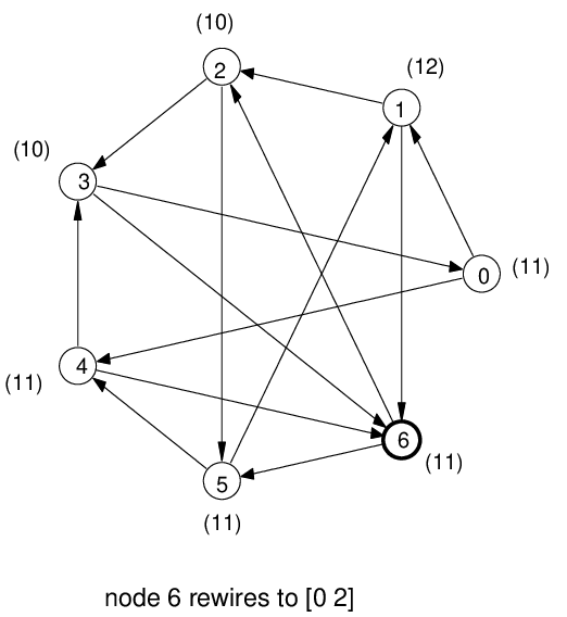


Unlike strong connectivity, convergence to a pure Nash equilibrium is not guaranteed. Next we show a simple example in which a round-robin best-reponse walk loops. Our simple example is on a (7,2)-uniform game that starts from the top-left configuration of Fig. 6. The nodes take turns in round-robin order, starting with node 6 then nodes 0,1,2, and so on. Tracing the example, one can verify that after 6 deviations (nodes re-wiring in this order, implying that missing nodes are stable), the graph returns to the initial configuration thus completing a loop.
The above example of a loop in the best response walk, does not rule out the possibility that either (a) a well-chosen best response walk converges from any initial state, or (b) certain best response walks do converge to stability if started from simple initial wirings such as the empty graph.
In order to address the preceding questions, we have conducted experiments on best response walks in large networks. We have discovered initial wirings for which the best response walk in which a node with the maximum cost always executes the best response step does not converge to a stable wiring. On the other hand, in all of our experiments, this best response walk always converges to a stable wiring, if started from an empty wiring.
Another closely related question is: From an empty wiring (or any initial wiring), is there a best-response walk of length polynomial in that leads to a pure Nash equilibrium? Our experiments suggest that from some initial wirings there might be an exponentially long best-response path to a pure Nash equilibrium.
In the first plot of Figure 7, we start round-robin best-response walk from a regular -wiring with offsets . All our experiments converge to a stable wiring. We plot the lengths of walks for all -pairs. In the second plot of Figure 7, we repeat the same experiment starting from a wiring constructed as follows: Starting from a simple directed Hamiltonian cycle, we add to every vertex random out-going links. Both experiments demonstrate lengthy and possible exponential convergence. Moreover, the “random” wiring experiment shows large variance in the length of convergence, especially for sparse wirings.
6 Open Problems
In this paper, we have proved that for any , the uniform Bounded Degree Network Formation (BDNF) Game always has a pure Nash equilibrium. In fact, the total social cost of our equilibrium is within a factor of 2 of the best possible network that could be constructed by a central network designer. In contrast, for non-uniform -BDNF games, a pure Nash equilibrium may not always exist. In fact, we show that deciding the existence of a pure Nash equilibrium is an NP-hard problem.
Several interesting and fundamental questions about the Bounded Degree Network Formation game remain open. Resolving them will be part of our future research. Here, we would like to discuss some of these questions and also state some conjectures inspired by our experiments.
Best-Response Paths to Pure Nash Equilibria
The first set of questions concerns the convergence of best-response walks. We would like to know whether the following statement is true.
- Q1
From every initial wiring of an -BDNF network, does there exist a best-response walk that leads to stable wiring?
In Section 5, we have given an example of an initial wiring from which some best-response walks induce a loop. But our example does not rule out a positive answer to Q1. There are several weaker statements about convergences that are worthy of further study.
- Q2
From every initial wiring of an -BDNF network, does there exist a strictly improving response-path that leads to a stable wiring?
- Q3
From an empty wiring, is there a round-robin best-response path that always leads to a stable wiring?
If the answer to Q1 is yes, an interesting follow-up question is the following.
- Q4
From every initial wiring of an -BDNF network, does there exist a best-response walk that leads to the stable graph constructed in Section 4.2?
Our experiments seem to suggest that there exists a best response walk that takes the empty wiring to the stable graph of Section 4.2 for . Note that if the answers to both Q1 and Q4 are yes, then the problem of finding a pure Nash equilibrium that is reachable by a best-response walk is not PLS-hard. Also, if best response walks indeed converge to stability, then resolving their convergence time is an important open problem.
Fairness vs Stability
The second set of the questions concerns the graph structure of stable uniform -wirings. Recall that a -wiring is completely fair if the costs of all vertices are the same. The following questions remains open:
- Q5
Is there a completely fair and stable -wiring for all and ?
We have shown that for , there exists an depending only on such that for all , there is no stable regular -wiring. This result inspires us to conjecture
Conjecture 1.
For every , there exists an depending on , such that for all , there is no completely fair and -stable graph.
A natural class of completely fair wirings is the class of vertex-transitive graphs. We have shown in Section 4.3 that a subclass of vertex transitive graphs, the Abelian Cayley graphs, are not stable for . Proving the following conjecture might be the first step to establish 1.
Conjecture 2.
For every , there exists depending on , such that for all , there is no vertex transitive directed graph over with out-degree .
Our experiments seems to suggest the following conjecture, which, provides a potential approach to settle Conjectures 1 and 2.
Conjecture 3.
For every , there exists depending on , such that for all , in every pure Nash equilibrium -wiring, all but vertices have in-degree .
References
- [1] Susanne Albers, Stefan Eilts, Eyal Even-Dar, Yishay Mansour, and Liam Roditty. On Nash equilibria for a network creation game. In Proc. of SODA ’06, pages 89–98, New York, NY, USA, 2006. ACM Press.
- [2] N. Alon and Y. Roichman. Random Cayley graphs and expanders. RSA: Random Structures & Algorithms, 5, 1994.
- [3] David Andersen, Hari Balakrishnan, Frans Kaashoek, and Robert Morris. Resilient overlay networks. In Proc. of ACM SOSP’01, Banff, Canada, Oct 2001.
- [4] F. Annexstein, M. Baumslag, and A. L. Rosenberg. Group action graphs and parallel architectures. SIAM Journal on Computing, 19:544–569, 1990.
- [5] Elliot Anshelevich, Bruce Shepherd, and Gordon Wilfong. Strategic network formation through peering and service agreements. In Proc. of IEEE FOCS ’06, pages 77–86, Washington, DC, USA, 2006.
- [6] Yatin Chawathe, Sylvia Ratnasamy, Lee Breslau, Nick Lanham, and Scott Shenker. Making Gnutella-like P2P systems scalable. In Proc. of ACM SIGCOMM ’03, pages 407–418, Karlsruhe, Germany, 2003.
- [7] G. Cooperman, L. Finkelstein, and N. Sarawagi. Applications of cayley graphs. In AAECC: Applied Algebra, Algebraic Algorithms and Error-Correcting Codes. LNCS, Springer-Verlag, 1990.
- [8] Jacomo Corbo and David C. Parkes. The price of selfish behavior in bilateral network formation. In Proc. of PODC’05, pages 99–107, 2005.
- [9] Alex Fabrikant, Ankur Luthra, Elitza Maneva, Christos H. Papadimitriou, and Scott Shenker. On a network creation game. In PODC ’03, pages 347–351, New York, NY, USA, 2003. ACM Press.
- [10] J. Feigenbaum, C. Papadimitriou, R. Sami, and S. Shenker. A bgp-based mechanism for lowest-cost routing. In PODC, 2002.
- [11] Elias Koutsoupias and Christos Papadimitriou. Worst-case equilibria. In STACS ’99, pages 404–413, March 1999.
- [12] Nikolaos Laoutaris, Georgios Smaragdakis, Azer Bestavros, and John Byers. Implications of selfish neighbor selection in overlay networks. In Proc. of IEEE INFOCOM ’07, Anchorage, AK, May 2007.
- [13] Yong Liu, Honggang Zhang, Weibo Gong, and Donald F. Towsley. On the interaction between overlay routing and underlay routing. In Proc. of IEEE INFOCOM ’05, pages 2543–2553, Miami, FL, 2005.
- [14] Qin Lv, Pei Cao, Edith Cohen, Kai Li, and Scott Shenker. Search and replication in unstructured peer-to-peer networks. In Proc. of ACM ICS ’02, pages 84–95, New York, NY, USA, 2002.
- [15] Evangelos Markakis and Amin Saberi. On the core of the multicommodity flow game. In Proc. of the 4th ACM conference on Electronic commerce, pages 93–97, New York, NY, USA, 2003. ACM Press.
- [16] Thomas Moscibroda, Stefan Schmid, and Roger Wattenhofer. On the topologies formed by selfish peers. In PODC ’06, 2006.
- [17] M.J. Osborne and A. Rubinstein. A Course in Game Theory. MIT Press, 1994.
- [18] Christos Papadimitriou. Algorithms, games, and the Internet. In STOC ’01, pages 749–753, New York, NY, USA, 2001. ACM Press.
- [19] Anthony Young, Jiang Chen, Zheng Ma, Arvind Krishnamurthy, Larry L. Peterson, and Randy Wang. Overlay mesh construction using interleaved spanning trees. In Proc of IEEE INFOCOM’04, Hong Kong, 2004.