In this work we deal with a mechanism for process simulation called a NonDeterministic Stochastic Activity Network (NDSAN). An NDSAN consists basically of a set of activities along with precedence relations involving these activities, which determine their order of execution. This order is captured by a digraph with some special properties: the possibility of defining nondeterministic branches of execution, by associating choice probabilities with some activities, and loops of execution, which specify the iterated execution of a group of activities according to predetermined loop probabilities. These properties allow for a rich variety of activity networks, capable of modeling many real situations in process engineering, project design, and troubleshooting.

There are two main types of activity networks. A deterministic activity network is represented by a precedence digraph whose topology remains fixed as the activities are executed. Examples of deterministic activity networks include CPM and PERT networks, see e.g. [10]. On the other hand, a nondeterministic activity network allows for the possibility of a dynamic topology. Examples of such networks are inhomogeneous Markov chains, GANs (Generalized Activity Networks) [4], and GERT (Graphical Evaluation and Review Technique) networks [11].

The duration of each network activity is given by a random variable. Thus, a fundamental problem is determining the distribution of the completion time of the entire network. For deterministic activity networks, this general problem is known as the Stochastic Project Scheduling Problem [3].

Our definition of NDSANs combines stochastic activity durations with nondeterminism. In an NDSAN, activities are represented by nodes, and an arc oriented from activity $a_{i}$ to activity $a_{j}$ means that the execution of $a_{j}$ may only start after the execution of $a_{i}$ has ended. Nondeterminism is achieved, as indicated above, by means of two possibilities: (i) some branches of execution are not necessarily taken, and (ii) the number of times a group of activities is to be executed is not determined a priori. These additional possibilities are supported by the introduction of two new categories of nodes, namely decision nodes and loop nodes. A decision node associates probabilities with its out-neighbors and selects one of them to be executed accordingly; this selection is interpreted as one possible deterministic scenario among many. A loop node allows the repeated execution of a group of activities, the number of iterations depending on probabilities associated with the loop node. Loop nodes are particularly interesting to model refinement processes, such as quality control and error testing/correction. We also define junction nodes for adequately combining the two new constructions into the network. In Section 2 we define NDSANs formally, in terms of recursive construction steps that combine smaller NDSANs into larger ones via certain types of structured templates.

In Section 3, we give an analytical description of the random variable $T[D]$ associated with the completion time of NDSAN $D$. We assume that the duration of each activity $a_{i}$ in $D$ is given by a continuous, nonnegative random variable $T_{i}$. The random variable $T[D]$ is thus given in terms of the $T_{i}$’s and the probabilities associated with the decision/loop nodes.

Although $T[D]$ can be described precisely, we lack a closed-form expression for it and even numerical methods to find its distribution from such a description may be computationally too hard, especially when the number of activities is large. In Section 4, we describe a recursive simulation algorithm whose execution returns a single plausible value (“observation”) in the sample space of $T[D]$. Running the simulation algorithm a suitable number $N$ of times produces a close approximation to the probability distribution of $T[D]$. The value of $N$ can be obtained by using the same statistic as the Kolmogorov-Smirnov test, see e.g. [7] (Section 13.5), as we also discuss in Section 4.

Section 5 presents two computational experiments. For each experiment, the result of the simulations is shown as a frequency histogram together with a fitting curve that approximates the expected shape of the density of $T[D]$, an approximate probability distribution of $T[D]$, and an approximate probability density of $T[D]$ obtained from the approximate distribution. Section 6 discusses ongoing work.

In a recent related work, Leemis et al. [9] develop algorithms to calculate the probability distribution of the completion time of a stochastic activity network with continuous activity durations. In their work, activities are modeled by arcs and the networks are acyclic and deterministic (i.e., allow no variation in topology). The authors describe a recursive Monte Carlo simulation algorithm, which is network-specific and must therefore be rewritten specifically for each new network. Also, they provide two exact algorithms, one for series-parallel networks and another for more general networks whose nodes have at most two incoming arcs each.

We remark that all the discussion on random variables in this work can be adapted to the case of discrete random variables. (In [13], pp. 122–123, for example, an activity network with discrete activity durations is given.)

In this work, $D$ denotes a digraph with $n$ nodes and $m$ arcs. If $(v,w)$ is an arc of $D$, then node $v$ is an in-neighbor of node $w$, whereas $w$ is an out-neighbor of $v$. By disregarding arc orientation, we may also simply say that $v$ and $w$ are neighbors. A node having no in-neighbors (resp. out-neighbors) is called a source node (resp. sink node). If $D$ is a digraph containing a single source (resp. sink) node $v$ , then $v$ is denoted by $source(D)$ (resp. $sink(D)$).

An NDSAN is a special digraph whose node set is partitioned into four subsets of nodes: a subset $S_{a}=\{a_{i}\mid 1\leq i\leq n_{a}\}$ of activity nodes; a subset $S_{b}=$ $\{b_{i}\mid 1\leq i\leq n_{b}\}$ of junction nodes; a subset $S_{d}=\{d_{i}\mid 1\leq i\leq n_{d}\}$ of decision nodes; and a subset $S_{\ell}=\{\ell_{i}\mid 1\leq i\leq n_{\ell}\}$ of loop nodes.

An activity node $a_{i}$ represents a single activity (or task) to be executed in the network. The execution of $a_{i}$ starts only after the execution of all of its in-neighbors has ended. When the execution of $a_{i}$ ends, all of its out-neighbors start executing simultaneously. Each activity node $a_{i}$ has a duration (execution time) $T_{i}$, which is a continuous, nonnegative random variable. We assume that the execution time of an activity node does not depend on the execution time of any other activity node. That is, the $T_{i}$’s are independent random variables. An activity node is represented by a circle. See Figure 1(a).

A junction node $b_{i}$ is used for a syntactic purpose. It may have several in-neighbors, but it has a single out-neighbor $v$. When the execution of any in-neighbor of $b_{i}$ ends, the execution of $v$ is started immediately. In other words, $b_{i}$ acts simply as a “connecting point” of incoming arcs. A junction node is represented by a square. See Figure 1(b).

A decision node $d_{i}$ is used to select one particular branch of the execution flow, as described in what follows. By construction, all of $d_{i}$’s neighbors are activity nodes. It has a single in-neighbor $a_{h}$ and $\alpha_{i}\geq 2$ out-neighbors $a_{j_{1}},\ldots,a_{j_{\alpha_{i}}}$. The execution of $d_{i}$ is assumed to be instantaneous, and consists of selecting exactly one of its out-neighbors, say $a_{j_{k}}$, as the next node to execute. The activity node $a_{j_{k}}$ is selected by $d_{i}$ with probability $p^{i}_{k}$, $k=1,\ldots,\alpha_{i}$, such that $\sum_{k=1}^{\alpha_{i}}p^{i}_{k}=1$. A decision node is represented by a lozenge. See Figure 1(c).

A loop node $\ell_{i}$ represents the usual iteration mechanism. By construction, $\ell_{i}$ has a single in-neighbor (a junction node $b_{h}$) and two out-neighbors (activity nodes $a_{r}$ and $a_{j}$). After the execution of $b_{h}$, a Boolean condition $E_{i}$ associated with $\ell_{i}$ is instantaneously tested: if $E_{i}$ is false then $a_{r}$ is executed next, otherwise $a_{j}$ is. An array of real values associated with ${\ell}_{i}$ gives the sequence $q^{i}_{1},\ldots,q^{i}_{\beta_{i}}$ of probabilities corresponding to $\beta_{i}$ consecutive passages through $\ell_{i}$, in such a way that the probability that $E_{i}$ is false at the $k$th passage through ${\ell}_{i}$ is $q^{i}_{k}$. That is, the probability of exiting the loop at this point is $1-q^{i}_{k}$. We assume that $q^{i}_{\beta_{i}}=0$ in order to guarantee the termination of the loop in at most $\beta_{i}$ consecutive passages through ${\ell}_{i}$. A loop node is represented by a filled lozenge. See Figure 1(d).

We are now ready to give the formal definition of NDSANs in terms of recursive construction steps. The base NDSAN is a digraph consisting of a single activity node. In a general step, NDSANs containing a single source node and a single sink node are combined to yield a larger NDSAN.

The recursive construction steps are based on the following Substitution Rule:

Substitution Rule: Let $D_{0}$ be a digraph and $\{v_{1},v_{2},\ldots,v_{\eta}\}$ a subset of its node set. Let $D_{1},D_{2},\ldots D_{\eta}$ be NDSANs, each containing a single source node and a single sink node. Construct an NDSAN $D$ by replacing $v_{i}$ by $D_{i}$, $1\leq i\leq\eta$, in such a way that every input (output) arc of $v_{i}$ in $D_{0}$ is an input (output) arc of $source(D_{i})$ ($sink(D_{i})$) in $D$. Let $Sub(D_{0},D_{1},\ldots,D_{\eta})=D$.

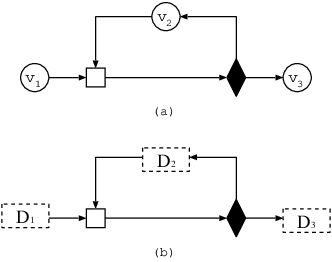
It is easy to see that the network $Sub(D_{0},D_{1},\ldots,D_{\eta})$ resulting from 2.1, 2.2, or 2.3 in the above definition contains a single source node and a single sink node, both activity nodes.

Scope of the definition of NDSANs. Although other definitions of NDSANs may be possible, we believe that Definition 1 not only determines a wide class of activity networks, but also allows the realization of any structured project, since it provides basic constructions that are generally thought to suffice for the specification of how concurrent tasks are to interrelate. In other words:

• –

  an acyclic NDSAN embodies the notion of multiple concurrent execution threads, which may be started as a single thread branches out into several independent ones, and terminated as they coalesce into a single thread for further execution.

• –

  a decision NDSAN allows for nondeterministic switches, or decision points, to be incorporated into the course of a thread’s execution.

• –

  a loop NDSAN allows any of the above to be iterated, possibly for a probabilistically selected number of times.

In this section we use the following terminology and notation. (See, for instance, [6, 7].) If $X$ is a random variable, then $F_{X}$ denotes the probability distribution function (PDF ) of $X$, and $f_{X}$ the probability density function (pdf ) of $X$. Recall that, for any $t$ in the domain of $X$, $F_{X}(t)=\mbox{Pr}(X\leq t)$. If $X$ is a continuous variable, we have

Hereafter, the random variable standing for the execution time of NDSAN $D$ will be denoted by $T[D]$. This random variable can be determined as follows.

Case 1: $D$ is a trivial NDSAN

Assuming that $D$ consists of the activity node $a_{i}$, we have $T[D]=T_{i}$.

Case 2: $D$ is not a trivial NDSAN

By 2.1, 2.2, and 2.3 in Definition 1, $T[D]$ can be recursively determined in terms of $T[D_{1}],T[D_{2}],\ldots,$ $T[D_{\eta}]$.

Case 2.1: $D$ is an acyclic NDSAN

Consider item 2.1 in Definition 1. Let ${\cal P}$ be the collection of all directed paths from $source(D_{0})$ to $sink(D_{0})$. Let $P\in{\cal P}$, and write $P=v_{i_{1}}v_{i_{2}}\ldots v_{i_{|P|}}$, where $|P|$ denotes the number of nodes of $P$. Let $D_{i_{1}},D_{i_{2}},\ldots,D_{i_{|P|}}$ be the NDSANs that substitute for $v_{i_{1}},v_{i_{2}},\ldots,v_{i_{|P|}}$. If $S_{P}$ is the time required for the serial execution of $D_{i_{1}},D_{i_{2}},\ldots,D_{i_{|P|}}$, then

(Recall that $T[D_{i_{k}}]$ is the random variable standing for the execution time of $D_{i_{k}}$, $1\leq k\leq|P|$.)

Since the $T[D_{i_{k}}]$’s are independent random variables, the pdf $f_{S_{P}}$ of $S_{P}$ is given by the convolution of the pdfs $f_{T[D_{i_{1}}]},f_{T[D_{i_{2}}]},\ldots,f_{T[D_{i_{|P|}}]}$, that is,

Define $f_{1}=f_{T[D_{i_{1}}]}$ and $f_{k}=f_{k-1}*f_{T[D_{i_{k}}]}$, $2\leq k\leq|P|$. Then we have, for any $t$,

Following Equation (1), the PDF of $S_{P}$ is then given by

Having described the variables $S_{P}$ for $P\in{\cal P}$, the random variable $T[D]$ is given by their maximum:

We remark that the variables $S_{P}$ are not independent, because two distinct paths in ${\cal P}$ may have nodes in common. Hence the PDF of $T[D]$ is given by

but no further simplification is in general possible. To determine the pdf of $T[D]$, simply apply Equation (1):

Case 2.2: $D$ is a decision NDSAN

In Figure 3(b), assume that the decision node is $d_{i}$. Then $\alpha_{i}=\eta-2$ and each node $source(D_{k})$ is selected by $d_{i}$ with probability $p^{i}_{k}$, $k=2,3,\ldots,\eta-1$. Let $X_{i}$ be a random variable associated with $d_{i}$ in such a way that

Then, clearly,

In order to proceed, note that the events $X_{i}=T[D_{k}]$, $2\leq k\leq\eta-1$, are mutually disjoint, since they correspond to disjoint subdigraphs of $D$. We then have

and

Thus,

and, by Equation (1),

Case 2.3: $D$ is a loop NDSAN

In Figure 4(b), assume that the loop node is $\ell_{i}$. For simplicity, assume also that $\beta_{i}=\beta$. Recall that, at the $k$th passage through ${\ell}_{i}$, the execution flow returns to $source(D_{2})$ with probability $q^{i}_{k},k=1,\ldots,\beta$, where $q^{i}_{{}_{\beta}}=0$ and $\beta$ is the maximum number of consecutive passages allowed through $\ell_{i}$.

Let $Z_{k}$ be the random variable standing for the total execution time of $k$ serial independent executions of $D_{2}$. Clearly, $Z_{k}$ is the sum of $k$ independent random variables, each one having distribution identical to that of $T[D_{2}]$. Therefore, $f_{Z_{k}}$ and $F_{Z_{k}}$ can once again be determined respectively by convolution and subsequent integration.

Consider now a random variable $Y_{i}$ associated with $d_{i}$ and such that

where the events $Y_{i}=0,\ Y_{i}=Z_{1},\ \ldots,\ Y_{i}=Z_{\beta-1}$ are all mutually disjoint. Then

and the functions $f_{T[D]}$ and $F_{T[D]}$ can be obtained as in Case 2.2, since the definition of $Y_{i}$ in Equation (15) has the same structure as that of $X_{i}$ in Equation (9).

Given an NDSAN $D$, obtaining the distribution and density functions of the target random variable $T[D]$ numerically may be an extremely costly computational task, even in simple cases. We refer the reader once again to the work by Leemis et al. [9], where even small networks are seen to need an elaborate mathematical analysis.

Our efforts are then directed toward seeking an approximate distribution of $T[D]$ within some required confidence level. We base our approach on collecting a random sample formed by a suitable number $N$ of independent observations of $T[D]$. Let us denote such an approximate distribution by $F^{{}^{N}}_{T[D]}$. Once $F^{{}^{N}}_{T[D]}$ is obtained, a frequency histogram and an approximate density $f^{{}^{N}}_{T[D]}$ can be easily determined, as we discuss later.

First, we present a simulation algorithm that, on input $D$, outputs a single observation $t$ of the sample space of $T[D]$. Next, we deal with the question of how many times the simulation algorithm must be repeated in order to obtain $F^{{}^{N}}_{T[D]}$ as required.

References

- [1] J. Blazewicz, J. K. Lenstra, and A. H. G. Rinnooy Kan. Scheduling subject to resource constraints: classification and complexity. Discrete Applied Mathematics 5 (1983) 11–24.
- [2] E. Demeulemeester, W. Herroelen, and B. De Reyck. A classification scheme for project scheduling. In J. Weglarz (ed.), Project Scheduling: Recent Models, Algorithms and Applications, Kluwer, Dordrecht, 1999, pp. 1–26.
- [3] E. Demeulemeester, W. Herroelen, and M. Vanhoucke. Discrete time/cost trade-offs in project scheduling with time-switch constraints. Journal of the Operational Research Society 53,7 (2002) 741–751.
- [4] S. E. Elmaghraby. Activity Networks, Wiley, New York, 1977.
- [5] M. Evans, N. Hastings, and B. Peacock. Statistical Distributions, 3rd ed., Wiley, New York, 2000, pp. 187–188.
- [6] W. Feller. An Introduction to Probability Theory and Its Applications, Vol. I, 2nd ed., Wiley, New York, 1991.
- [7] P. G. Hoel. Introduction to Mathematical Statistics, 3rd ed., Wiley, New York, 1965.
- [8] D. E. Knuth. The Art of Computer Programming, Vol. II, 3rd ed., Addison-Wesley, Reading, Massachusetts, 1997.
- [9] L. M. Leemis, M. J. Duggan, J. H. Drew, J. A. Mallozzi, and K. W. Connel. Algorithms to calculate the distribution of the longest path length of a stochastic activity network with continuous activity durations. Networks 48 (2006) 143–165.
- [10] J. J. Moder, C. R. Phillips, and E. W. Davis. Project Management with CPM, PERT and Precedence Diagramming. Van Nostrand Reinhold Company, New York, 3rd ed., 1983.
- [11] L. J. Moore and E. R. Clayton. GERT Modeling and Simulation: Fundamentals and Applications. Petrocelli/Charter, New York, 1976.
- [12] R. A. V. Olaguibel and J. M. T. Goerlich. Heuristic algorithms for resource-constrained project scheduling. In R. Slowinski and J. Werglarz (eds.), Advances in Project Scheduling, Elsevier, Amsterdam, 1989, pp. 113–134.
- [13] D. R. Shier. Network Reliability and Algebraic Structures. Oxford University Press, New York, 1991.
- [14] B. W. Silverman. Density Estimation for Statistics and Data Analysis. Chapman & Hall, London, 1986.
- [15]
E. W. Weisstein.
Log normal distribution.
Wolfram MathWorld,
http://mathworld.wolfram.com/LogNormalDistribution.html.