Efficient Threshold Aggregation of Moving Objects

Scot Anderson Email: sanderson@southern.edu Affiliation: Southern Adventist University, Tennessee Peter Revesz Email: revesz@cse.unl.edu Affiliation: University of Nebraska-Lincoln

Abstract

Calculating aggregation operators of moving point objects, using time as a continuous variable, presents unique problems when querying for congestion in a moving and changing (or dynamic) query space. We present a set of congestion query operators, based on a threshold value, that estimate the following $5$ aggregation operations in $d$ -dimensions. 1) We call the count of point objects that intersect the dynamic query space during the query time interval, the CountRange. 2) We call the Maximum (or Minimum) congestion in the dynamic query space at any time during the query time interval, the MaxCount (or MinCount). 3) We call the sum of time that the dynamic query space is congested, the ThresholdSum. 4) We call the number of times that the dynamic query space is congested, the ThresholdCount. And 5) we call the average length of time of all the time intervals when the dynamic query space is congested, the ThresholdAverage. These operators rely on a novel approach to transforming the problem of selection based on position to a problem of selection based on a threshold. These operators can be used to predict concentrations of migrating birds that may carry disease such as Bird Flu and hence the information may be used to predict high risk areas. On a smaller scale, those operators are also applicable to maintaining safety in airplane operations. We present the theory of our estimation operators and provide algorithms for exact operators. The implementations of those operators, and experiments, which include data from more than 7500 queries, indicate that our estimation operators produce fast, efficient results with error under 5%.

1 Introduction

Safety can often be reduced to to a problem of congestion. The safety of flight depends on separation of airplanes or more generally the maximum number of airplanes that a particular airspace can safely contain, and the maximum number of airplanes that air traffic controllers (ATC) responsible for directing airplanes can safely track. When considering epidemics, the presence of a single animal with Bird Flue does not does not indicate the start of an epidemic. Instead the presence of a certain number of instances of the disease indicates a high risk of starting an epidemic, or actual epidemic conditions. Consequently, we see that congestion often links to safety and can predict high risk or even dangerous conditions.

Congestion is defined differently depending on the application. Hence it is necessary to provide aggregation operators that take a threshold value as a parameter to define congestion.

In relational databases, Max, Min, Count, Sum and Average form the set of natural aggregation-operators. Spatiotemporal databases containing moving objects, based on continuous time, can not apply these operators in the same way. However, these operators may still function in interesting ways for moving objects. For example, one can ask how many moving point objects exist within a moving and changing (or dynamic) rectangular area at a certain time, or what is the maximum distance between two moving points at certain times. Obviously, when we are interested in discrete time instances, then the moving point object database can be reduced to a relational database and the above queries can be expressed as simple Count or Max queries.

Moving object databases naturally suggest new aggregate operators that have no equivalents in relational databases. For example, one may ask what is the maximum number of moving-point objects that exist simultaneously within a dynamic rectangular area at any time during a time interval $T$ ? We call this the MaxCount query (symmetrically we can also find the Min-Count). One may also ask during what time intervals in $T$ does there exist more than $M$ moving objects within a rectangular area? We call this the ThresholdRange. We show that a strong relationship exists between MaxCount and ThresholdRange, and we show that ThresholdRange forms the bases for a family of threshold operators that include: ThresholdCount, ThresholdSum, and ThresholdAverage. A related, though less complex, operator answers the question: what is the number of moving objects that exist within or intersect a dynamic rectangular area at any time instance during interval $T$ . We call this type of query the CountRange query.

We give the following definitions for aggregation operators:

Definition 1 (Dynamic Query Space)

Dynamic query space is defined by a continuous time interval $T$ , and a $d$ -dimensional space that may move and change size or shape over the query time interval.

Throughout this paper we consider the shape of the query space to be a box or cube.

Definition 2 (MaxCount (MinCount))

Let $S$ be a set of moving points. Given a dynamic query space $R$ defined by two moving points $Q_{1}$ and $Q_{2}$ as the lower-left and upper-right corners of $R$ , and a time interval $T$ , the MaxCount (Min-Count) operator finds the time $t_{\max(\min)}$ and maximum (or minimum) number of points $M_{\max(\min)}$ in $S$ that $R$ can contain at any time instance within $T$ .

Throughout this paper we develop the MaxCount operator because where ever we find a maximum, a minimum can be found similarly.

Definition 3 (ThresholdRange)

Let $S$ be a set of moving points. Given a dynamic query space $R$ defined by two moving points $Q_{1}$ and $Q_{2}$ as the lower-left and upper-right corners of $R$ , a time interval $T$ , and a threshold value $M$ , the ThresholdRange operator finds the set of time intervals $T_{M}$ where the count of objects in $R$ is larger than $M$ .

ThresholdRange is directly related to MaxCount in that when $M$ is raised to $M_{\max}$ , then ThresholdRange returns a time interval containing $t_{\max}$ and during this time interval, the count will be $M_{\max}$ .

Definition 4 (ThresholdCount)

Given a ThresholdRange, ThresholdCount returns the number of time intervals.

Definition 5 (ThresholdSum)

Given a ThresholdRange, ThresholdSum returns the total time $T_{s}$ during which the count is above $M$ . That is, for each $T_{i}\in T_{M}$ , ThresholdSum return:

T_{s}=\displaystyle{\sum\limits_{i}}|T_{i}|

(1)

where $|T_{i}|$ means the length of the interval.

Definition 6 (ThresholdRange)

Given a ThresholdRange, ThresholdAverage returns the average length of the intervals in $T_{M}$ .

In addition to the threshold aggregation operators, we also use our bucketing method to implement the CountRange defined as follows.

Definition 7 (CountRange)

Let $S$ be a set of moving points. Given a dynamic query space $R$ defined by two moving points $Q_{1}$ and $Q_{2}$ as the lower-left and upper-right corners of $R$ and a time interval $T$ , the CountRange query returns the total number of points that intersect $R$ in $T$ .

Together MaxCount (MinCount) and the threshold operators form a complete set of threshold aggregation operators comparable to the aggregation operators given in relational databases.

The following examples use the simple concepts of flying to demonstrate the use of a few of these threshold aggregation operators.

Example 8

Airplanes are commonly modeled as linearly moving objects with preestablished flight plans. Suppose, at any time, at most a constant number $M$ of airplanes is allowed to be in the O’Hare airspace to avoid congestion. Suppose also a new airplane requests approval of its flight plan for entering the O’Hare airspace between times $t_{a}$ and $t_{b}$ . The air traffic controllers can avoid congestion as follows. If after adding a new flight plan, the MaxCount between $t_{a}$ and $t_{b}$ is still less than $M$ , then they can approve the flight. Otherwise, they need to find some alternative path, and check it again against the database.

Air traffic controllers try to direct airplanes as linearly moving objects for fuel efficiency, among other reasons. If they recognize a developing congestion too late, then they often must direct the airplane to fly in circles until the congestion has cleared. That solution wastes fuel. On the other hand, if they recognize the developing congestion early, then they can often simply tell the airplane to change its speed, which saves fuel. Therefore, it is important to identify congestions as early as possible. We may identify congestions by using a MaxCount query where a moving box around the airplane and a time interval $[t_{a},t_{b}]$ define the query. If the MaxCount predicts congestion, then the airplane’s speed can be adjusted early in the flight.

Example 9

Suppose we want to alert pilots if their current flight path takes them through at least one congested region.

Traffic Alert/Collision Avoidance Systems (TCAS) is a system that provides similar functionality. TCASs only provide alerts for current congestion, not predictive congestion. Although TCASs were implemented in 1986, we continue to have mid-air collisions and near misses indicating that the system still needs improvement. ThresholdRange is a modification of MaxCount that returns all predicted time intervals on the flight path where the Count exceeds a given threshold. Hence using ThresholdRange we can alert a pilot of predicted congestions where more than $M$ other airplanes will be within the space $B$ around the airplane. Predicting and avoiding these areas can significantly reduce the chances of mid-air collisions.

Example 10

Suppose we are especially concerned about a rush-hour period $[t_{a},t_{b}]$ that is particularly stressful to air traffic controllers. Suppose controllers can direct at most $M$ airplanes safely. We can determine the number of controllers needed during the rush-hour time by executing the CountRange query over the controlled airspace during the rush-hour and dividing by $M$ . By ensuring that a sufficient number of controllers are present, safety is achieved and controllers are not over stressed.

Each of the operators can also be applied to examine different aspects of congestion with regard to bird migration and hence disease control. These questions and examples, motivated by research on MaxCount, led us to explore complex threshold aggregations and data structures to support them.

The rest of this paper is organized as follows. Section 2 gives some background on the concepts of point domination, sweeping techniques and then introduces the data structures used to build buckets. These buckets can then be used in various indexing algorithms to fit the type of application used. Section 3 develops the MaxCount estimation algorithm using a running example. Section 4 develops the ThresholdRange algorithm based on MaxCount and demonstrates the relationship that ties MaxCount to the remaining threshold operators. This section also develops algorithms for each of those operators including CountRange. Section 5 gives the experimental results of the implementation. Section 6 reviews the related work and Section 7 gives conclusions and future work.

2 Hyper-Bucket Data Structures

This section presents an updatable skew-aware bucket for indices that models the skewed point distributions in each bucket. The skew-aware technique allows the index structure to perform inserts, deletes, and updates in fast constant time using a HashTable to store the buckets. Many spatiotemporal applications, such as tracking clients on a wireless network, particularly need these fast updates and no other MaxCount presented prior to this can meet that requirement. Because the buckets are spatially defined, the bucketing technique also easily adapts to other spatial and spatiotemporal indices such as the R-tree Guttman 1984. Hence the technique performs well for applications where search operations or update operations occur more frequently by using an appropriate index.

Our algorithm uses a sweeping method to evaluate the threshold aggregation operators similar to previous approaches from Chen & Revesz 2004; Revesz & Chen 2003 and Anderson 2006. The algorithm differs in that the sweeping algorithm integrates a skew-aware density function over the spatial dimensions of the bucket to obtain the time dependent count function. The density function in the bucket increases accuracy over methods given in (Chen & Revesz 2004; Anderson 2006) while maintaining the same number of buckets. This idea is a crucial improvement because we model the point distribution skew in a bucket, whereas previous methods adapted to skew by increasing the number of buckets or changing their shape and contents. We also present a precise algorithm for evaluating the threshold aggregation operators that requires no index and runs in $O(N)+O(n\log n)$ time and $O(n)$ space where $N$ is the number of points in the database and $n$ is the value of a CountRange query using the same query space and time. Both the threshold aggregation algorithms and the skew-aware bucket data structure presented are implemented and analyzed in 3-dimensional space. We show that the approximation achieves good results while significantly reducing the running times.

Section 2.1 describes the problems related to creating hyper-buckets (also referred to as just buckets) and a specific solution for creating $6$ -dimensional buckets for $3$ -dimensional linearly moving points. In all cases, we can extend our method to $d$ -dimensions. Section 2.2 describes the method for inserting and deleting a point from a bucket and shows that updates take constant time. Section 2.3 applies two different data structures to contain the buckets suited for applications where either inserts and deletes or threshold aggregation queries dominate.

2.1 Hyper-Bucket Data Structure

Definition 11 (Hex Representation)

Define each 3-dimensional linearly moving point $p$ by parametric linear equations in $t$ as follows:

p=\left\{\begin{array}[]{c}p_{x}~=~v_{x}t~+~x_{0}\\ p_{y}~=~v_{y}t~+~y_{0}\\ p_{z}~=~v_{z}t~+~z_{0}\\ \end{array}\right.

(2)

where the corresponding hex representation of $p$ is the tuple $(v_{x},x_{0},v_{y},y_{0},v_{z},z_{0})$ containing the duals of $p_{x}$ , $p_{y}$ , and $p_{z}$ . For simplicity we often denote the six-tuple as $(x_{1},...,x_{6})$ .

Consider a relation $D(x_{1},..,x_{6})$ that contains the hex representation of linearly moving points in $3$ dimensions. Then $D$ represents a $6$ -dimensional static space. Divide the space into axis-aligned hyper-rectangles where the $k^{th}$ axis has $d_{k}$ divisions. Each hyper-rectangle becomes a bucket containing moving points whose hex falls inside the hyper-rectangle.

Definition 12 (Hyper-bucket dimensions)

Define the dimensions of each bucket $B_{i}$ by inequalities of the form:

\begin{array}[]{lcl}v_{x,L}\leq v_{x}<v_{x,U}&\bigwedge&x_{0,L}\leq x_{0}<x_{0,U}~\bigwedge\\ v_{y,L}\leq v_{y}<v_{y,U}&\bigwedge&y_{0,L}\leq y_{0}<y_{0,U}~\bigwedge\\ v_{z,L}\leq v_{z}<v_{z,U}&\bigwedge&z_{0,L}\leq z_{0}<z_{0,U}\\ \end{array}

(3)

where we denote the lower bound as:

(v_{x,L},x_{0,L},v_{y,L},y_{0,L},v_{z,L},z_{0,L})

(4)

and the upper bound as

(v_{x,U},x_{0,U},v_{y,U},y_{0,U},v_{z,U},z_{0,U}).

(5)

Each hyper-rectangle defines the spatial dimensions of a possible bucket, where only buckets that contain points need be included in the index. The maximum number of possible buckets is given by $m=\prod\limits_{k}d_{k}$ .

Definition 13 (Histograms)

Given a $6$ -dimensional rectangle $B_{i}$ , given by Definition 12, containing $b_{i}$ points, build the histograms $h_{i,1}$ ,…, $h_{i,6}$ for each axis using $s$ subdivisions as follows. To create histogram $h_{i,j}$ , divide bucket $B_{i}$ into $s$ parallel subdivisions along the $j$ th axis, and record separately the number of points within $B_{i}$ that fall within each subdivision.

Example 14 (Building Histograms)

Refer to caption — Figure 1: Points projected onto $v_{x},x_{0}$ plane.

Consider a set of 6-dimensional points projected onto the $v_{x},x_{0}$ plane as shown in Figure 1. Assume that the number of subdivisions is $s=10$ along both $v_{x}$ and $x_{0}$ . Figure 2 shows $h_{i,1}$ and $h_{i,2}$ . For example, the subdivision $0\leq v_{x}<1$ contains six points and hence the first bar of histogram $h_{i,1}$ rises to level $6$ . The other values can be determined similarly.

Histograms tell much about the distribution of the points in a bucket but they introduce some ambiguity. For example, the histograms in Figure 2 match both of the $2d$ -distributions in Figure 3.

Definition 15 (Axis Trend Function)

The axis trend function $f_{i,j}(x_{j})$ is some polynomial function for bucket $B_{i}$ and axis $j$ such that the following hold:

1.

$f_{i,j}\geq 0$ over $B_{i}$ .
2.

$f^{\prime}_{i,j}$ , the derivative $f_{i,j}$ , does not change sign over the valid range.

The bucket trend function $f_{i}$ for bucket $B_{i}$ is the following:

f_{i}=\prod_{j}f_{i,j}

(6)

Condition 1 ensures that the bucket trend function, built from the axis trend functions, does not contain a negative probability region. Condition 2 requires that the bucket density increase, decrease, or remain constant when considering any single axis. This condition avoids the ambiguity demonstrated in Figures 2 and 3 by giving a polynomial that approximates the density change correctly. We show this in the following Lemma.

Lemma 16

Given a bucket $B_{i}$ with bucket trend functions $f_{i,j}$ , let $r_{1}$ and $r_{2}$ be identically sized regions in bucket $B_{i}$ . If the density in $B_{i}$ along each axis monotonically increases from $r_{1}$ to $r_{2}$ the following holds:

\int_{r_{2}}f_{i}~d\phi\geq\int_{r_{1}}f_{i}~d\phi

(7)

Proof. Increasing densities from $r_{1}$ to $r_{2}$ translates into histograms that also increase from $r_{1}$ in the direction of $r_{2}$ along each axis. The translation from histograms to the axis trend functions gives the following conditions:

f_{i,j}(x_{2,j})\geq f_{i,j}(x_{1,j})

(8)

where $x_{1,j}$ and $x_{2,j}$ are the $j^{th}$ coordinates of the points in $r_{1}$ and $r_{2}$ respectively, and are located the same distance from the $j^{th}$ coordinates of the lower bounds of $r_{1}$ and $r_{2}$ respectively. Since this constraint holds for each $j$ and $f_{i,j}\geq 0$ we have:

f_{i}(x_{2})\geq f_{i}(x_{1})

(9)

Hence by the properties of integration we conclude

\int_{r_{2}}f_{i}~d\phi\geq\int_{r_{1}}f_{i}~d\phi

(10)

Definition 15 allows a whole class of polynomial functions, and Lemma 16 applies to each member of that class. However, in the following, we use a particular polynomial function derived from the product of linear functions, which are obtained by using the least squares method for each histogram.

Definition 17 (Normalized Trend Functions)

Let $n$ be the number of points in the database, $b_{i}$ the number of points in bucket $B_{i}$ , and $f_{i}$ be given by Equation (6). The normalized trend function $F_{i}$ for bucket $B_{i}$ is:

F_{i}=\frac{b_{i}f_{i}}{n\mathop{\displaystyle\int}\limits_{B_{i}}^{~}f_{i}~d\phi}

(11)

and the percentage of points in bucket $B_{i}$ is:

p=\mathop{\displaystyle\int}\limits_{B_{i}}F_{i}~d\phi.

(12)

With this definition we can calculate the number of points in $O(1)$ time using the following simple lemma.

Lemma 18

Let $B_{i}$ be a bucket, $n$ the number of points in the databases, and $p$ be given by Definition 17. Then $np$ is the number of points in bucket $B_{i}$ and $np$ is calculated in $O(1)$ time.

Proof. By Equation (11) and (12) we have:

\begin{array}[]{ccl}np&=&n\mathop{\displaystyle\int}\limits_{B_{i}}F_{i}~d\phi\\ &=&n\mathop{\displaystyle\int}\limits_{B_{i}}\displaystyle{\frac{b_{i}}{n}}\frac{f_{i}}{\mathop{\displaystyle\int}_{B_{i}}f_{i}~d\phi}~d\phi\\ &=&n\displaystyle{\frac{b_{i}}{n}}\cdot\frac{\mathop{\displaystyle\int}_{B_{i}}f_{i}~d\phi}{\mathop{\displaystyle\int}_{B_{i}}f_{i}~d\phi}\\ &=&b_{i}.\\ \end{array}

(13)

Clearly the above calculations take only $O(1)$ time.

Using the above definitions we can now define the bucket data structure used throughout the rest of this paper.

Definition 19 (Skew Aware Buckets)

A bucket is a hyper-rectangle with dimensions given by Definition 12 and that maintains histograms given by Definition 13, additional data for the least squares method, and the normalized trend function given by Definition 17. Throughout the rest of this paper we refer to these as buckets.

2.2 Inserts and Deletes

We can maintain the bucket (and hence the index) while deleting or inserting a point for any bucket $B_{i}$ by recalculating the trend function $F_{i}$ for the bucket.

Lemma 20

Insertion and deletion of a moving point can be done in $O(1)$ time.

Proof. When we insert or delete a point, we need to update the histograms and the normalized trend function. Let the point to insert/delete be $P_{a}$ represented using the hex representation as $(a_{0},a_{1},a_{2},a_{3},a_{4},a_{5})$ , let $d_{j}$ , for $0\leq j\leq 5$ be the bucket width in the $j^{th}$ , and let $s$ be the number of subdivisions in each histogram. The concatenation of $id_{0},\ldots,id_{5}$ gives the $ID_{i}$ of bucket $i$ to insert (or delete) $P_{a}$ into where each $id_{l}$ and $0\leq l\leq 5$ is defined by:

id_{l}=\left\lfloor\frac{a_{l}}{d_{l}}\right\rfloor.

(14)

The calculation of $ID_{i}$ and retrieving bucket $B_{i}$ takes $O(1)$ time using a HashTable.

Let $hw_{i,j}$ be the histogram-division width for the $j^{th}$ calculated as $hw_{i,j}=\left\lceil\frac{d_{j}}{s}\right\rceil$ . Then $p$ is projected onto each dimension to determine which division of the histogram to update. For the $j^{th}$ dimension the $k^{th}$ division of histogram $h_{i,j}$ is given as follows:

k(j)=\left\lfloor\frac{a_{j}-id_{j}*d_{j}}{hw_{k}}\right\rfloor

(15)

Let $h_{i,j,k}$ be the histogram division to update for each histogram. Update $h_{i,j,k}$ and the sums $\displaystyle{\sum}y_{i}$ , and $\displaystyle{\sum}x_{i}y_{i}$ from the normal equations in the least squares method. $N$ , $\displaystyle{\sum}x_{i}$ and $\displaystyle{\sum}x_{i}^{2}$ from the normal equations do not need updating since the number of histogram divisions $s$ is fixed within the database.

We can now recalculate each $f_{i,j}$ in constant time by solving the $2\times 3$ matrix corresponding to the normal equations of the least squares method for each histogram. For each $f_{i,j}$ calculate the endpoints to determine the required shift amount (Definition 15, property 1) and calculate $f_{i}$ from Equation (6). Now we calculate $F_{i}$ using Equation (17). Each of these steps depends only on the dimension of the database. Hence for any fixed dimension we can rebuild the normalized trend function $F_{i}$ in $O(1)$ time.

2.3 Index Data Structures

There is no need to create a bucket unless it contains at least one point. We consider two classes of data structures for organizing the buckets: HashTables and Trees.

For databases where inserts and deletes are the most common operation, the HashTable approach allows these operations to run in constant time. However, the MaxCount operation will require an enumeration of all the buckets and thus at least a running time of $O(B)$ . As long as the number of buckets is reasonable, this approach works well.

For databases where MaxCount is the most common operation, we may use an R-tree structure (Guttman 1984; Beckmann et al. 1990) where the elements to be inserted are the buckets. This approach speeds up the MaxCount query to $O(\log|B|+R)$ where $R$ is the number of buckets needed to calculate the query. The insert and delete costs for these R-trees are $O(\log|B|)$ , because buckets do not overlap.

Since buckets do not change shape, the database is decomposable and allows each type of aggregation to be calculated from simultaneous executions on subspaces of the index space. We discuss the method and ramifications of this capability at the end of Section 3.4.

3 Dynamic MaxCount

Section 3.1 reviews point domination in higher dimensions. Section 3.2 examines finding the percentage of points in a bucket that are in the query space as a function of time. Section 3.3 puts the two previous sections together to create the dynamic MaxCount algorithm for $d$ -dimensions.

3.1 Point Domination in 6-Dimensional Space

Let $B$ be the set of 6-dimensional hyper-buckets in the input where each hyper-bucket $B_{i}$ has an associated normalized trend function $F_{i}$ as in Definition 17. Let the vertices of $B_{i}$ be denoted $v_{i,j}$ where $1\leq j\leq 64$ , because there are $2^{6}$ corner vertices to a 6-dimensional hyper-cube.

Definition 21 (Point Domination)

Given two linearly moving points in three dimensions

P(t)=\left\{\begin{array}[]{l}p_{x}=x_{1}t+x_{2}\\ p_{y}=x_{3}t+x_{4}\\ p_{z}=x_{5}t+x_{6}\end{array}\right.\quad{\rm and}\quad Q(t)=\left\{\begin{array}[]{l}q_{x}=v_{x}t+x_{0}\\ q_{y}=v_{y}t+y_{0}\\ q_{z}=v_{z}t+z_{0}\end{array}\right.

(16)

$Q(t)$ dominates $P(t)$ if and only if the following holds:

(p_{x}<q_{x})\quad\wedge\quad(p_{y}<q_{y})\quad\wedge\quad(p_{z}<q_{z}).

(17)

The previous definition takes 6-dimensional points defined in Definition 11 and places them into three inequalities of the form $x_{2}<-t(x_{1}-v_{x})+x_{0}$ . Each inequality defines a region below a line with slope $-t$ .

Definition 22 ( $x$ -view, $y$ -view and $z$ -view projections)

Projecting the inequalities from Definition 21 onto their respective dual planes allows a visualization in three 2-dimensional planes. Define these three projections as the $x-$ view, $y-$ view and $z-$ view respectively. Because the time $-t$ defines the slopes of each line, all views contain lines with identical slopes. (See Figure 4)

Definition 23 (Query Space)

Given two moving query points $Q_{1}(t)$ and $Q_{2}(t)$ and lines $l_{x1}$ , $l_{x2}$ , $l_{y1}$ , $l_{y2}$ , $l_{z1}$ , $l_{z2}$ crossing them in their respective hexes with slopes $-t$ , the intersection of the bands formed by the area between $l_{x1}$ and $l_{x2}$ , $l_{y1}$ and $l_{y2}$ , and $l_{z1}$ and $l_{z2}$ in the 6-dimensional space forms a hyper-tunnel that defines the query space as shown in Figure 4.

We can now visualize the query in space and time as the query space sweeping through a bucket as the slopes of the lines change with time. Using the above, it is now easy to prove the following lemma.

Lemma 24

At any time $t$ , the moving points whose hex-representation lies below (or above) $l_{x1},l_{y1}$ and $l_{z1}$ in their respective views are exactly those points that lie below (or above) $Q_{1}$ in the original 3-dimensional plane.

Proof. Let $Q_{x}(t)=v_{x}t+x_{0}$ where $v_{x}$ and $x_{0}$ are constants and consider any $x$ component of a point $P_{x}(t)=x_{1}t+x_{2}$ that lies below $Q$ on the $x$ -axis. Then

	$\displaystyle x_{1}t+x_{2}$	$\displaystyle<$	$\displaystyle v_{x}t+x_{0}$		(18)
	$\displaystyle x_{2}$	$\displaystyle<$	$\displaystyle-t(x_{1}-v_{x})+x_{0}$		(19)

Obviously, at any time $t$ these are the points below the line $x_{2}=-t(x_{1}-v_{x})+x_{0}$ , which has a slope of $-t$ and goes through $(v_{x},x_{0})$ . This representation is the dual of point $Q_{x}$ . By Definition 23, this is exactly the line $l_{x1}$ . We can prove similarly that the points with duals above $l_{x1}$ are above $Q_{1}$ at any time $t$ . The proof that points whose hex-representations are above or below $l_{y1},$ and $l_{z1}$ are exactly those points that lie above or below $Q_{1}$ is similar to the proof for points above or below $l_{x1}$ . By Definition 21, we conclude that the points dominated by $Q_{1}$ in the dual space are those points that are below $l_{x1},l_{y1}$ , and $l_{z1}$ in the $x$ -view, $y-$ view, and $z$ -view, respectively. Similarly, we conclude that the points that dominate $Q_{1}$ in the dual space are those points that are above $l_{x1},~l_{y1}$ , and $l_{z1}$ in the $x$ -view, $y-$ view, and $z$ -view, respectively.

Throughout the examples in this chapter, we use the points shown in Figures 5 and 6 to demonstrate the evaluation of a MaxCount query. We begin by creating the index.

Example 25 (Creating the Index)

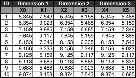
Consider a relation that contains the $6$ -dimensional space 10 units $(0\ldots 10)$ in each dimension. If we break this up into buckets that are $5$ units long in each dimension, we have $2^{6}$ buckets. Although these divisions make a space with $64$ buckets, all the points are contained in a single bucket whose index is $(2,2,2,2,2,2)$ . All the points listed in Figure 5 have the same velocities for each dual plane. Notice the columns for $x_{1}$ , $x_{3}$ , and $x_{5}$ all have the same values in different orders. The projection of the points onto the $3$ dual planes shown in Figure 6 does not immediately show this organization. Projecting the points for any view in Figure 7 onto each axis and creating histograms with $5$ divisions gives the histograms for the Velocity and Position axes shown in Figure 7.

Hence, each velocity dimension has the same histogram. Similarly each position dimension has the same histogram. To create these histograms each point is projected onto the axis. For example point $1$ projected onto the $x_{1}$ axis is given as:

~5.345,7.543,5.345,8.158,5.345,5.488\rightarrow 5.345.

(20)

Calculate the widths of the histograms as:

Histogram\_Width=(10-5)/5=1

(21)

We determine the histogram for each point by looping through the points and calculating the following:

division=\left\lfloor((point-lowerbound)/Histogram\_Width)\right\rfloor

(22)

For example the lowest and highest points in velocity would be added to the division calculated as $\left\lfloor\left(5.84-5\right)/1\right\rfloor=0$ and $\left\lfloor(9.468-5)/1\right\rfloor=4$ .

The histograms translate into a set of points for each view given as:

	$\displaystyle Velocity=\{(0,1),(1,1),(2,2),(3,2),(4,4)\}$		(23)
	$\displaystyle Position=\{(0,2),(1,2),(2,2),(3,2),(4,2)\}$		(24)

Before applying the least squares method each division number must be translated back into the bucket. Translation is done using the following code fragment:

for $i\leftarrow 0$ to number_of_divisions $-1$
	$point[i][0]\ \leftarrow i*histogram\_width+lowerbound$
	$point[i][1]\ \leftarrow histogram\_value[i]$
end for

Translation of the points from (23) and (24) gives: The histograms for velocity and position in each view are given as:

	$\displaystyle Velocity=\{(5,1),(6,1),(7,2),(8,2),(9,4)\}$		(25)
	$\displaystyle Position=\{(5,2),(6,2),(7,2),(8,2),(9,2)\}.$		(26)

Using the least squares method to fit each of these to a line yields the following for each velocity and position dimension:

	$\displaystyle Velocity:~~$	$\displaystyle y=0.7x-2.9$		(27)
	$\displaystyle Position:~~$	$\displaystyle y=0x+2.$		(28)

Evaluating Equations (27) and (28) at the end points to find the shift value for the axis trend function to add to each equation gives:

	$\displaystyle Velocity:~~$	$\displaystyle y(5)=1,~~y(10)=4.3$		(29)
	$\displaystyle Position:~~$	$\displaystyle y(5)=y(10)=2.$		(30)

In this case no constant needs to be added to our equation and the trend function becomes:

f_{i}=(0.7x_{0}-2.9)(0x_{1}+2)(0.7x_{2}-2.9)(0x_{3}+2)(0.7x_{4}-2.9)(0x_{5}+2)

(31)

Calculating $F_{i}$ from Equation (11) requires integrating $f_{i}$ over the bucket where $\int_{B_{i}}\equiv\int_{5}^{10}...\int_{5}^{10}$ and where $d\phi\equiv dx_{0}dx_{1}dx_{2}dx_{3}dx_{4}dx_{5}$ gives

	$\displaystyle\int_{B_{i}}f_{i}d\phi$	$\displaystyle=8\int_{B_{i}}(0.7x_{0}-2.9)(0.7x_{2}-2.9)(0.7x_{4}-2.9)d\phi$
		$\displaystyle=1622234.375.$		(32)

Since all the points reside in a single bucket, $b_{i}=n$ , the constant $c$ is given by $c=1/1622234.375\approx 6.164\times 10^{-7}$ . Then $F_{i}$ is given by

	$\displaystyle F_{i}$	$\displaystyle\approx c~(0.7x_{0}-2.9)(0x_{1}+2)(0.7x_{2}-2.9)(0x_{3}+2)(0.7x_{4}-2.9)(0x_{5}+2)$
		$\displaystyle=8c(0.7x_{0}-2.9)(.7x_{2}-2.9)(.7x_{4}-2.9)$		(33)

So far we have calculated the normalized trend function $F_{i}$ for just one bucket. This calculation finishes the bucket creation process, and the index contains this single bucket defined by the points $lowerbound=(5,5,5,5,5,5)$ and $upperbound=(10,10,10,10,10,10)$ .

3.2 Approximating the Number of Points in a Bucket

As a line through a query point sweeps across a bucket, the points in the bucket that dominate the query point are approximated by the integral over the region above the line. In each of the three views the query space intersects the plane giving the cases shown in Figure 8.

Definition 26 (Percentage Function)

Integrating over the region above the line gives an approximation of the percentage of points in the query space. We define the percentage function given as:

p=\int\limits_{r_{1}}F_{i}~d\phi

(34)

where $r_{1}$ is the region of the bucket in the query space. If two lines go through the same bucket we have the smaller region $r_{2}$ subtracted from the larger region $r_{1}$ as follows.

\triangle p=\int\limits_{r_{1}}F_{i}~d\phi-\int\limits_{r_{2}}F_{i}~d\phi.

(35)

Here, regions $r_{1}$ and $r_{2}$ correspond to regions above $Q_{1}$ and $Q_{2}$ in Figure 4, respectively. Lemma 18 showed that finding the number of points in the bucket requires multiplying Equation (34) or (35) by $n$ .

For each case shown in Figure 8, we describe the function that results from integration in one view. To extend the result to any number of views, we take the result from the last view and integrate it in the next view. If the region below the line were desired, $p_{lower}=\frac{b_{i}}{n}-p$ gives the percentage of points below the line.

For cases (a) – (h) below, let $Q=(x_{1,q},x_{2,q},...,x_{6,q})$ . For the $x$ -view, let the lower left corner vertex be $(x_{1,l},x_{2,l})$ and the upper right corner vertex be $(x_{1,u},x_{2,u})$ . In addition each line denoted $l$ is given by $x_{2}=-t(x_{1}-x_{i,q})+x_{i+1,q}$ and corresponds to a line shown in the corresponding case in Figure 8.

Case (a): For this case $l$ crosses the bucket at $x_{1,l}$ and $x_{2,u}$ . The integral over the shaded region is given by the following:

p_{a}=\int\limits_{x_{1,l}}^{\frac{x_{2,u}-x_{2,q}}{-t}+x_{1,q}}\int\limits_{-t(x_{1}-x_{1,q})+x_{2,q}}^{x_{2,u}}F_{i}~dx_{2}dx_{1}

(36)

Notice that the lower bound of the integral over $dx_{2}$ contains $x_{1}$ . This dependence within each view does not affect the integration in the remaining four dimensions. The solution to Equation (36) has the form:

at^{2}+bt+c+\frac{d}{t}+\frac{e}{t^{2}}.

(37)

Case (b): For this case $l$ crosses the bucket at $x_{1,u}$ and $x_{2,u}$ . The integral over the shaded region is given by:

p_{b}=\int\limits_{-\frac{(x_{2,u}-x_{2,q})}{t}+x_{1,q}}^{x_{1,u}}\int\limits_{-t(x_{1}-x_{1,q})+x_{2,q}}^{x_{2,u}}F_{i}~dx_{2}dx_{1}.

(38)

The solution has the form of Equation (37).

Case (c): For this case $l$ crosses the bucket at $x_{1,l}$ and $x_{2,l}$ . The integral over the shaded region above the line is given by:

p_{e}=\int\limits_{x_{1,l}}^{\frac{x_{2,l}-x_{2,q}}{-t}+x_{1,q}}\int\limits_{-t(x_{1}-x_{1,q})+x_{2,q}}^{x_{2,u}}F_{i}~dx_{2}dx_{1}~+~\int\limits_{\frac{x_{2,l}-x_{2,q}}{-t}+x_{1,q}}^{x_{1,l}}\int\limits_{x_{2,l}}^{x_{2,u}}F_{i}~dx_{2}dx_{1}.

(39)

The solution has the form of Equation (37).

Case (d): For this case $l$ crosses the bucket at $x_{1,u}$ and $x_{2,l}$ . The integral over the shaded region is given by:

p_{f}=\int\limits_{\frac{x_{2,l}-x_{2,q}}{-t}+x_{1,q}}^{x_{1,u}}\int\limits_{-t(x_{1}-x_{1,q})+x_{2,q}}^{x_{2,u}}F_{i}~dx_{2}dx_{1}~+~\int\limits_{x_{1,l}}^{\frac{x_{2,l}-x_{2,q}}{-t}+x_{1,q}}\int\limits_{x_{2,l}}^{x_{2,u}}F_{i}~dx_{2}dx_{1}.

(40)

The solution has the form of Equation (37).

Case (e): For this case $l$ crosses the bucket at $x_{1,l}$ and $x_{1,u}$ . The integral over the shaded region is given by:

p_{c}=\int\limits_{x_{2,l}}^{x_{2,u}}\int\limits_{x_{1,l}}^{\frac{x_{2}-x_{2,q}}{-t}+x_{1,q}}F_{i}~dx_{1}dx_{2}.

(41)

The solution has the form of

c+\frac{d}{t}+\frac{e}{t^{2}}

(42)

which is like Equation (37) with $a=b=0$ .

Case (f): Similar to case(e), $l$ crosses the bucket at $x_{1,l}$ and $x_{1,u}$ . The integral over the shaded region is given by:

p_{d}=\int\limits_{x_{2,l}}^{x_{2,u}}\int\limits_{\frac{x_{2}-x_{2,q}}{-t}+x_{1,q}}^{x_{1,u}}F_{i}~dx_{1}dx_{2}.

(43)

The solution has the form of Equation (42).

Case (g): For this case $l$ crosses the bucket at $x_{1,l}$ and $x_{1,u}$ . The integral over the shaded region is given by:

p_{g}=\int\limits_{x_{1,l}}^{x_{1,u}}\int\limits_{-t(x_{1}-x_{1,q})+x_{2,q}}^{x_{2,u}}F_{i}~dx_{2}dx_{1}.

(44)

The solution has the form

at^{2}+bt+c

(45)

which is like Equation (37) with $d=e=0$ .

Case (h): The line $l$ crosses below all the corner vertices hence the integral of the function is given as:

p_{h}=\int\limits_{x_{1,l}}^{x_{1,u}}\int\limits_{x_{2,l}}^{x_{2,u}}F_{i}~dx_{2}dx_{1}.

(46)

The solution has the form of Equation (45).

The above cases have solutions for each view in the form of Equation (37). Hence the percentage function for a single bucket as a function of $t$ is of the form:

	$\displaystyle p$	$\displaystyle=\left(a_{x}t^{2}+b_{x}t+c_{x}+\frac{d_{x}}{t}+\frac{e_{x}}{t^{2}}\right)\left(a_{y}t^{2}+b_{y}t+c_{y}+\frac{d_{y}}{t}+\frac{e_{y}}{t^{2}}\right)$
		$\displaystyle~~~~\left(a_{z}t^{2}+b_{z}t+c_{z}+\frac{d_{z}}{t}+\frac{e_{z}}{t^{2}}\right)$		(47)

where $t\neq 0$ when $d_{x},d_{y},d_{z},e_{x},e_{y},e_{z}\neq 0$ . Finally, renaming variables gives the general form:

p=a_{6}t^{6}+a_{5}t^{5}+a_{4}t^{4}+a_{3}t^{3}+a_{2}t^{2}+a_{1}t+c+\frac{d_{1}}{t}+\frac{d_{2}}{t^{2}}+\frac{d_{3}}{t^{3}}+\frac{d_{4}}{t^{4}}+\frac{d_{5}}{t^{5}}+\frac{d_{6}}{t^{6}}

(48)

where $t\neq 0$ when $d_{i}\neq 0$ for $1\leq i\leq 6$ . Since Equation (48) is closed under subtraction, $\triangle p$ from Equation (35) will also have the same form.

As the query space from Definition 23 sweeps through a bucket, it crosses the bucket corner vertices. Each time a corner vertex crosses the query space boundary, the case that applies may change in one or more of the views.

Definition 27 (Bucket and Index Time-Intervals)

The span of time in which no vertex from bucket $B_{i}$ enters or leaves the query space defines a bucket time-interval. We denote the time-interval as a half-open interval $[l,u)$ where $l$ is the lower bound and $u$ is the upper bound. Each bucket time-interval has an associated percentage function $\triangle p$ given by Equation (35). We define the index time-interval similarly except that the span of time is defined when no vertex from any bucket in the index enters or leaves the query space.

As we will see, index time-intervals are created from individual bucket intervals. Throughout the rest of this dissertation we use the term time intervals when the context clearly identifies which type we mean.

Definition 28 (Time-Partition Order)

Let $B$ be the set of buckets. Let $Q_{1}$ and $Q_{2}$ be two query points and $(t^{[},t^{]})$ be the query time interval. We define the Time-Partition Order to be the set of ordered time instances $TP={t_{1},t_{2},...,t_{i},...,t_{k}}$ such that $t_{1}=t^{[}$ and $t_{k}=t^{]}$ , and each $[t_{i},t_{i+1})$ is an index time-interval.

Example 29 (Calculating Bucket Time-Intervals)

Continuing Example 25, let $Q$ be a query defined by:

$\displaystyle q_{1}$	$\displaystyle=$	$\displaystyle(9.5,~8,~9.5,~8,~9.5,~8)$	(49)
$\displaystyle q_{2}$	$\displaystyle=$	$\displaystyle(8.5,~5,~8.5,~5,~8.5,~5)$	(50)
$\displaystyle T$	$\displaystyle=$	$\displaystyle(0.1,~10)$	(51)

where $q_{1}$ and $q_{2}$ form the query space over the query time interval $T$ . To determine time intervals when corner vertices do not change, find the slopes of lines through both query points and each corner vertex of the bucket. Figure 9 shows lines from the two query points to the corner vertices for the first dimension. Since the query points are the same in each dimension each will appear the same.

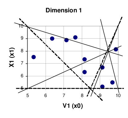
The set of times when lines through $q_{1}$ (shown as solid lines) cross corner vertices is $\{0.\overline{4},6\}$ . The set of times when lines through $q_{2}$ (shown as dotted lines) cross corner vertices and are in the time interval is $\{1.42857\}$ . The union of these two sets along with the end points makes up the times used to create the time intervals: $\{(.1,0.\overline{4}),(0.\overline{4},1.42857),(1.42857,6),(6,10)\}$ .

Integration over the spatial dimensions of the eight possible cases presented in Figure 8 gave a function of the form of Equation (48). Maximizing Equation (48) in the temporal dimension by first taking the derivative, we get:

	$\displaystyle\triangle p^{\prime}$	$\displaystyle=$	$\displaystyle(6a_{6}t^{12}+5a_{5}t^{11}+4a_{4}t^{10}+3a_{3}t^{9}+2a_{2}t^{8}+a_{1}t^{7}$		(52)
			$\displaystyle~-d_{1}t^{5}-2d_{2}t^{4}-3d_{3}t^{3}-4d_{4}t^{2}-5d_{5}t-6d_{6})/t^{7}$		(52)

where $t\neq 0$ . Solving $\triangle p^{\prime}=0$ requires finding the roots of this $12$ -degree polynomial, which is not possible using an exact method. Hence we need a numerical method for solving the polynomial.

The following factors influenced the choice of the numerical method:

1.

Speed of the algorithm is more important than accuracy because we don’t expect the original function to change dramatically over an index time-interval. We expect small change because in practice the time intervals are short.
2.

The algorithm must converge toward a solution within the interval, that is the algorithm must be stable.
3.

Given that we are maximizing Equation (48) over a short time interval, we don’t expect Equation (52) to have more than one solution. This assumption may seem naive, but it is reasonable given factor (1).

Factor (1) above is related to (3) in that it indicates that points close together have similar values, but emphasizes that speed is the goal. Factor (2) above eliminates several algorithms from consideration, but must be required to keep from choosing a solution that is not within the time interval evaluated.

Of the three points to consider, (3) is probably the least intuitive. Consider the following conjecture:

Conjecture 30

Given $p$ for a set of buckets, if the Euclidean distance between two maxima is small, then the difference between the maxima is small.

Consider the physical characteristics of the system. The value of $p$ over the time interval changes no more than $b_{i}$ for any bucket $B_{i}$ . Clearly $p$ either increases as it encompasses more of the bucket or decreases at as it encompasses less of the bucket. When $p$ represents the distribution over several buckets, each bucket contributes a decreasing or increasing amount over the time interval. Clearly $p$ is bounded below by $0$ and above by $\sum\limits_{i}b_{i}$ . Hence, the rate at which the derivative $p^{\prime}$ changes is characterized by the physical system and reflects the differences in the buckets as $t$ changes. Since $p$ does not change dramatically over $t$ for any bucket, then change in several buckets over $t$ will likewise not be dramatic. Hence if the distance between two maxima is small, the maxima have a small difference in magnitude. This rational for the conjecture above is verified by the experiments.

Based on these factors, we use a common method for the first approximation: we look at the graph of $p^{\prime}$ . Programmatically check $c$ intervals of Equation (52) for a change in sign. If there exists a sign change, use the bisection method to find the root. If two points lie within $\epsilon$ of $0$ , we perform a check for each of these intervals when no change of sign is found. If some roots exist, we check them for maximal values along with the end points.

Lemma 31

The approximate maximum within a time interval can be found in $O(1)$ time.

Proof. Each time interval has an associated probability function $\triangle p$ which is calculated in $O(1)$ time. Finding $\triangle p^{\prime}=0$ also takes $O(1)$ time. By placing a constant bound on the number of iterations in the bisection method, we bound the time required in the numerical section of the algorithm by a constant. Plugging in the solution found by the bisection method along with the end points also takes $O(1)$ time. Hence, the running time to find the maximum within a bucket is $O(1)$ .

We chose to limit the number of iterations in the bisection method to 10, which limits the running time to a small constant value. This value was chosen based on empirical observation that index time-intervals remain small (about $0.01$ to $4$ ). Hence, using the bisection method allows us to narrow our search down to an interval at least as small as $\frac{1}{256}$ units of time. If time is measured in hours, this interval equates to only $14$ seconds.

Example 32 (Building Time-Intervals and Finding MaxCount)

Continuing Example 29 we build the functions for time intervals

\{(.1,0.\overline{4}),(0.\overline{4},1.42857),(1.42857,6),(6,10)\}

(53)

by integrating using the different cases from Figure 8. For space concerns we omit the integrals here and note that the result of integrating each interval and finding the maximum gives a maximum of approximately $3$ at $t=0.\overline{4}$

Time Interval: $[0.1,0.\overline{4}]$ . Here case (c) holds for query point $q_{2}$ over this time interval. Hence the integral for query point $q_{2}$ and $t\in[.1,.\overline{4}]$ in each dimension is given as:

	$\displaystyle p_{c}$	$\displaystyle=$	$\displaystyle c\int_{8.5}^{10}\int_{5}^{10}2(0.7x_{0}-2.9)dx_{1}dx_{0}+\int_{5}^{8.5}\int_{-t(x_{0}-8.5)+5}^{10}2(0.7x_{0}-2.9)dx_{1}dx_{0}$		(54)
		$\displaystyle=$	$\displaystyle 117.5-17.354\bar{6}t$		(54)

Case (g) holds for query point $q_{1}$ and thus the integral for query point $q_{1}$ and $t\in(.1,.\overline{4})$ in each dimension is given as:

	$\displaystyle p_{g}$	$\displaystyle=c\int_{5}^{10}\int_{-t(x_{0}-9.5)+8}^{10}2(0.7x_{0}-2.9)dx_{1}dx_{0}$
		$\displaystyle=47.0-32.41\bar{6}t$		(55)

Hence the integral of the region is:

	$\displaystyle p$	$\displaystyle=c\left(p_{c}-p_{g}\right)^{3}$
		$\displaystyle=2.106\times 10^{-3}t^{3}+2.957\times 10^{-2}t^{2}+0.138t+0.216$		(56)

Evaluating $p$ at the start and end of the time interval we have $p(0.1)\approx 0.23$ and $p(0.\overline{4})=0.28$ . Figure 10 shows $p$ in the time interval. Clearly $p$ is increasing and consequently we have a maximum at the end point $t=0.\overline{4}$ .

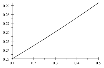
Since there are $10$ points we must multiply $p(0.\overline{4})$ by $10$ to get the approximation for the time interval as:

MaxCount_{0.1\leq t\leq 0.\overline{4}}\approx 2.8.

(57)

Since we can not have partial points, we can round this result to $3$ .

The rest of the intervals are similar using different cases. We omit the remaining cases to save space and to eliminate the risk of boring the reader. None of the other intervals has a higher MaxCount and so it follows that MaxCount has an approximate value of $3$ at time $t=0.\overline{4}$ .

3.3 Dynamic MaxCount Algorithm

MaxCount $(H,Q_{1},Q_{2},t^{[},t^{]})$
input:		A set of buckets $H$ built by the index structure presented,
		query points $Q_{1}(t)$ and $Q_{2}(t)$ and a query time interval $(t^{[},t^{]})$ .
output:		The estimated MaxCount value.

01.	$TimeIntervals\leftarrow\emptyset$ $O(1)$
02.	for $i\leftarrow 0$ to $\|H\|-1$ $O(B)$
03.		$CrossTimes\leftarrow$ CalculateCrossTimes $(Q_{1},Q_{2},t^{[},t^{]},H_{i})$ $O(1)$
04.		for $j\leftarrow 1$ to $\|CrossTimes\|-1$ $O(1)$
05.			Union $(TimeIntervals,TimeInterval(t_{j-1},t_{j})$ $O(1)$
06.		end for
07.	end for

08.	$TimeIntervals=$ BucketSort $(TimeIntervals)$ $O(B)$
09.	$IndexTimeIntervals=$ Merge $(TimeIntervals)$ $O(B)$
10.	for each $IndexTimeInterval\in IndexTimeIntervals$ $O(B)$
11.		calculate $(MaxCount,MaxTime,IndexTimeInterval)$ $O(1)$
12.	end for

13.	return $(MaxCount,MaxTime)$

The algorithm to compute MaxCount with each line labeled with its running time is given above. Line 01 initiates a set of bucket time-interval objects to be empty. Line 03 returns a list of ordered times when a line through $Q_{1}$ or $Q_{2}$ crosses a bucket corner vertex. Line 05 turns this list into a set of $TimeInterval$ objects and adds them to the set of $TimeIntervals$ . We list this “for each” loop as $O(1)$ because it consists of a constant number of calculations bounded by the number of vertices in the bucket. Line 08 uses the linear time sorting algorithm BucketSort to sort the bucket time intervals. Line 09 creates the time-partition order and index bucket time intervals from the bucket time intervals in $O(B)$ . An additional pass adds the bucket time intervals to the appropriate index time-intervals in $O(B)$ . Lines 10-12 perform the MaxCount calculation discussed above.

In order to use the linear time BucketSort algorithm, we need the following definition and lemmas.

Definition 33 (Time-Interval Ordering)

We define the lexicographical ordering $\prec$ of two time intervals $A$ and $B$ as follows:

$\displaystyle A.l<B.l$	$\displaystyle\Rightarrow$	$\displaystyle A\prec B$	(58)
$\displaystyle A.l=B.l\quad\wedge\quad A.u<B.u$	$\displaystyle\Rightarrow$	$\displaystyle A\prec B$	(59)
$\displaystyle A.l=B.l\quad\wedge\quad A.u=B.u$	$\displaystyle\Rightarrow$	$\displaystyle A=B$	(60)

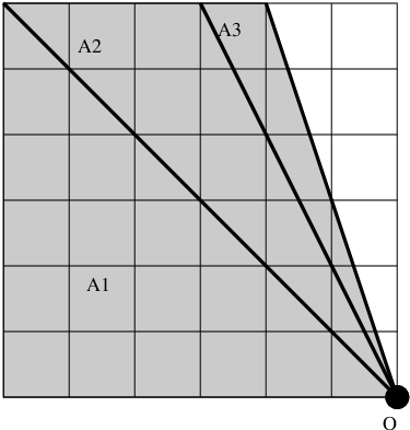
The distribution of time interval objects created in Line 08 of the MaxCount algorithm may not be uniform across the query time interval $T=[t^{[},t^{]}]$ . However, we can still prove the following.

Lemma 34

If the distribution of buckets is uniform, then the distribution of bucket time-interval objects can be uniformly distributed within the sorting buckets of the bucket sort.

Proof. Consider the relationship between successive slopes measured as the angles between lines through a query point $Q$ with slopes $s_{i}=-t_{i}$ and $s_{i+1}=-t_{i+1}$ . Suppose $\triangle t=1$ with $t_{0}=0$ and $t_{1}=1$ , then the angle between the two lines is $\triangle s=\frac{\pi}{4}$ . The solid lines in Figure 11 show that half of the bucket corner vertices are swept by the line sweeping through $Q$ between $s_{0}=0$ and $s_{1}=-1$ . Consider a query time interval $[0,10]$ . Half of the corner vertices, and thus half of the time intervals, are between time $t=0$ and $t=1$ . Thus, we conclude that the time interval objects created by sweeping will not be uniformly distributed throughout the query time interval.

Let $Q^{\prime}$ be the midpoint between $Q_{1}$ and $Q_{2}$ . Let $S=\{t_{1},...t_{k}\}$ where $t_{1}=t^{[}$ , $t_{k}=t^{]}$ and $t_{i+1}-t_{i}=L$ for some positive constant $L$ and $1\leq i\leq k-1$ . Let $D_{B}$ be a bucket that contains the space in the 6-dimensional index. Model the normalized bucket function for $D_{B}$ as a constant $F=1$ . Thus $p$ , the bucket probability, from Equation (3.2) becomes the hyper-volume of the space swept by the line through $Q^{\prime}$ . By Lemma 31, we can find the area for a specific time interval in $S$ in constant time. The percentage of sorting buckets, $posb_{i}$ , needed in any time interval $T_{i}=[t_{i},t_{i+1}]\in S$ within the query time interval is given by:

posb_{i}=\frac{p(t_{i+1})-p(t_{i})}{p(t^{]})-p(t^{[})}

(61)

Let $N$ be the number of sorting buckets. Then, the number of sorting buckets, $nosb_{i}$ , assigned to interval $i$ is given by:

nosb_{i}=N\cdot posb_{i}

(62)

If $nosb_{i}<1$ we can combine it with $nosb_{i+1}$ . If the query time interval is very large, then we may need to include multiple time intervals from $S$ to get one sorting bucket. Thus, we create more sorting buckets (with smaller time intervals) in areas where the expected number of bucket time intervals is large. Conversely, we create fewer sorting buckets (with larger time intervals) in areas where the expected number of bucket time intervals is small. Hence we model each sorting bucket so that its time interval length directly relates to the percentage of bucket time intervals that are assigned to it. Thus, we conclude that we will uniformly distribute the time interval objects across all sorting buckets.

Lemma 35

Insertion of any bucket time-interval object $T_{O}$ into the proper sorting bucket can be done in $O(1)$ time.

Proof. The distribution of sorting buckets is determined by $k$ time intervals in Lemma 34. Call these sorting time interval objects where each object contains: the lower bound $l$ , the upper bound $u$ , the number of sorting buckets assigned to this interval $b_{s}$ , the length of the time interval for the sorting bucket $w$ and an array $B_{p}$ containing pointers to these sorting buckets. Let $A$ be the array of sorting time interval objects, and $L$ be the length of each time interval where the time intervals are as in Lemma 34. Then, finding the correct sorting bucket for $T_{O}$ requires two calculations:

	$\displaystyle SortingTimeInterval$	$\displaystyle=$	$\displaystyle A\left[~\left\lfloor\frac{T_{O}.l}{L}\right\rfloor~\right]$		(63)
	$\displaystyle SortingBucket$	$\displaystyle=$	$\displaystyle B_{p}\left[~\left\lfloor\frac{T_{O}.l-SortingTimeInterval.l}{w}\right\rfloor~\right].$		(64)

Each of these calculations requires constant time, hence $T_{O}$ can be inserted into the proper sorting bucket in $O(1)$ time.

Using the above two lemmas, we can prove the following.

Theorem 36

The running time of the MaxCount algorithm is $O(B)$ where $B$ is the number of buckets.

Proof. Let $H$ be the set of buckets where each bucket $B_{i}$ contains the normalized trend function $F_{i}$ . Let $Q_{1}$ and $Q_{2}$ be the query points and $[t^{[},t^{]}]$ be the query time interval. (Lines 01-07): Calculating the time intervals takes $O(B)$ time because the cross times for each bucket can be calculated in constant time. (Line 08): By Lemmas 34 and 35, we have an approximately even distribution of time interval objects within the sorting buckets where we can insert an object in constant time. This result fulfills the requirements of the BucketSort, Cormen et al. 2001, which allows the intervals to be sorted in $O(B)$ time. (Lines 09-12): Calculate the MaxCount and time for each time interval in constant time using Lemma 31. These lines takes $O(B)$ time because there are $O(B)$ time intervals. Finding the global MaxCount and time requires retaining the maximum time and count at line 11. Returning the MaxCount and time takes $O(1)$ time. Thus, the running time is given by $O(B)+O(B)+O(B)+O(1)=O(B)$ .

3.4 An Exact MaxCount Algorithm

The Exact MaxCount algorithm below finds the exact MaxCount values. It is easy to see that the running time is given by:

O(N)+O(n\log n)

(65)

where $N$ is the number of points in the database and $n$ represents the result size of the query.

It is possible to slightly improve the algorithm below. First, divide the index space into $k$ subspaces and maintain separate partial databases for each. Assign processes on individual systems to each database to calculate the MaxCount query and return the time intervals to a central process. Merging the time interval lists into a global time interval list saves time on the sorting part of the algorithm. The running time for each of $k$ partial databases would be close to $O(\frac{n}{k}\log\frac{n}{k})$ . This result is an approximate value because we do not guarantee an even split between partial databases. Placing buckets for each partial database in a Tree structure may be reasonable and could cut down the average running time to $O(\log N+n\log n/k)$ . Implementation and analysis for this particular approach is left as future work.

ExactMaxCount $(D,Q_{1},Q_{2},t^{[},t^{]})$
input:		$D$ is the database of points. The query is made up of a
		hyper-rectangle $Q$ defined by points $Q_{1}$ and $Q_{2}$ and the time
		interval $T=[t^{[},t^{]}]$
output:		The exact MaxCount and time at which it occurs.

01.	$Times\leftarrow\emptyset$ //of CrossTime objects $O(1)$
02.	for each point $p_{i}\in D$ $O(N)$
03.		if $p_{i}\in Q$ during $T$ $O(1)$
04.			$EntryTime\leftarrow CalculateEntryTime(p_{i},Q,T)$ $O(1)$
05.			$ExitTime\leftarrow CalculateExitTime(p_{i},Q,T)$ $O(1)$
06.			if $EntryTime\in Times$ $O(1)$
07.				$Times.$ get $(EntryTime).Count$ ++ $O(1)$
08.			else
09.				$Times.$ add $(newCrossTime(EntryTime))$ $O(1)$
10.			end if
11.			if $ExitTime\in Times$ $O(1)$
12.				$Times.$ get $(ExitTime).Count$ - - $O(1)$
13.			else
14.				$Times.$ add $(newCrossTime(ExitTime))$ $O(1)$
15.			end if
16.	end for
17.	Sort $(Times)$ $O(n\log n)$
18.	traverse $(Times,time,Max\textrm{-}Count)$ //tracking time $O(N)$
				//and MaxCount
19.	return (time,MaxCount) $O(1)$

4 Threshold Operators

ThresholdRange $(H,Q_{1},Q_{2},t^{[},t^{]},M)$
input:		A set of buckets $H$ build by the index structure presented,
		query points $Q_{1}(t)$ and $Q_{2}(t)$ , a query time interval $[t^{[},t^{]}]$ ,
		and $M$ is the threshold value
output:		The estimated set of time intervals where $R$ contains more
		than $M$ points.

01 - 08 are the same as the MaxCount algorithm.
09.	$TimeIntervals\leftarrow\emptyset$ $O(1)$
10.	for each $TimeInterval\in TimePartitionOrder$ $O(B)$
11.		$CMaxCount\leftarrow\textsc{calculate}(\textsc{MaxCount},MaxTime,TimeInterval)$ $O(1)$
12.		if $CMaxCount>M$ $O(1)$
13.			$TimeIntervals\leftarrow TimeIntervals\bigcup TimeInterval$ $O(1)$
14.		end if
15.	end for
16.	$\textsc{Merge}(TimeIntervals)$ $O(B)$
17.	return $TimeIntervals$

The ThresholdRange algorithm shown above and described in Definition 3 relates to MaxCount in the way we calculate the aggregation. We maintain a running count to find time intervals that exceed the threshold value $M$ . If we set the threshold value near the MaxCount value ( $M\rightarrow$ MaxCount), ThresholdRange finds a small interval containing the MaxCount. We demonstrate this in the experimental results, Section 5.

The ThresholdRange algorithm is the same as MaxCount up to Line 08, and then collects different information from each $TimeInterval$ starting in Line 10. This leads to the following Theorem.

Theorem 37

The estimated ThresholdRange query runs in $O(B)$ time.

Proof. The ThresholdRange algorithm differs from the MaxCount algorithm only in lines 09-17. Lines 11-14 run in $O(1)$ time. Line 10 executes lines 11-13 $O(B)$ times. In line 16, $\textsc{Merge}(TimeIntervals)$ is a linear walk of the time intervals that joins adjacent time intervals $T_{a}$ and $T_{b}$ when $T_{a}\bigcup T_{b}$ would form a continuous time interval. The calculation is trivially $O(1)$ time for joining the adjacent intervals. Hence, we conclude by Theorem 36 that the ThresholdRange runs in $O(B)$ time.

4.1 Threshold: Sum, Count and Average

We give the following three operators based on ThresholdRange and conclude that none of the changes to the algorithm affect the running time of the ThresholdRange algorithm.

ThresholdCount:
By adding a line between 14 and 15 in the ThresholdRange algorithm that counts the merged time intervals, we can return the count of time intervals during the query time interval where congestion occurs. This count of time intervals gives a measure of variation in congestion. That is, if we have lots of time intervals, we expect that we have a large number of pockets of congestion. Since ThresholdCount does not give information relative to the entire time interval, it may need to be examined in light of the total time above the threshold.

ThresholdSum:
By summing the times instead of using the $\bigcup$ operator in line 13 of the ThresholdRange algorithm, we can return the total congestion time during the query time interval. This total gives a measure of the severity of congestion that may be compared to the length of query time.

ThresholdAverage:
By adding a line between lines 14 and 15 in the ThresholdRange algorithm that finds average length of the merged time intervals, we can return the average length of time each congestion will last. This average gives a different measure of the severity of each congestion.

4.2 Count Range Algorithm

The CountRange algorithm is an adaptation of MaxCount in that it is the Count portion of the MaxCount query. Using the equations for the cases described in Figure 8, we calculate the CountRange as follows:

For each bucket we determine if the bucket is completely in or completely out of the query space. First we find the beginning and ending time intervals. For each time interval, we get the associated function $\triangle p$ given in Equation (35) and its components. The components $\triangle p$ given in Equation (34) define the area above a line through $Q_{1}$ and $Q_{2}$ at times $t^{[}$ and $t^{]}$ . Figures 13 and 13 show these four lines. Figure 13 shows the shaded area defined by:

\triangle\overleftarrow{p}=p_{Q_{2},t^{[}}-p_{Q_{1},t^{]}}.

(66)

Figure 13 shows the shaded area:

\triangle\overrightarrow{p}=p_{Q_{2},t^{]}}-p_{Q_{1},t^{[}}.

(67)

If $\triangle\overleftarrow{p}$ or $\triangle\overrightarrow{p}$ for bucket $i$ is equal to the count of the bucket, then bucket $i$ is completely contained in the query. If $\triangle\overleftarrow{p}$ and $\triangle\overrightarrow{p}$ for bucket $i$ are equal to $0$ , then bucket $i$ is not contained in the query. If neither of these is true, we approximate the count for bucket $i$ as the $\max(\triangle\overleftarrow{p},\triangle\overrightarrow{p})$ . That is, we calculate the number of points in bucket $i$ that contribute to the CountRange as:

count_{i}=\left\{\begin{array}[]{llr}b_{i}&\textrm{ if }&\triangle\overleftarrow{p}=b_{i}\vee\triangle\overrightarrow{p}=b_{i}\\ 0&\textrm{ if }&\triangle\overleftarrow{p}=\triangle\overrightarrow{p}=0\\ \max(\triangle\overleftarrow{p},\triangle\overrightarrow{p})&&\textrm{ Otherwise}\end{array}\right.

(68)

This calculation requires that we keep the single dimension equations for $Q_{1}$ and $Q_{2}$ available and not discard them after finding $\triangle p$ (see Equation (35)).

Hence, we have the following algorithm for CountRange:

CountRange $(H,Q_{1},Q_{2},t^{[},t^{]})$
input:		A set of buckets $H$ built by the index structure presented,
		query points $Q_{1}(t)$ and $Q_{2}(t)$ and a query time interval $(t^{[},t^{]})$ .
output:		the estimated CountRange.

1.	$Count\leftarrow 0$ $O(1)$
2.	for each bucket $B_{i}\in D$ $O(B)$
3.		Calculate( $\triangle\overleftarrow{p},\triangle\overrightarrow{p}$ ) //using Equations (66)-(67) $O(1)$
4.		Calculate( $count_{i}$ ) //using Equation (68) $O(1)$
5.		$Count\leftarrow Count+count_{i}$ $O(1)$
6.	end for
7.	return $Count$ $O(1)$

Theorem 38

The CountRange query runs in $O(B)$ time.

Proof. Consider two different data structures for our buckets: HashTables and R-trees. In the case of indexing using an R-tree, the worst case requires that we examine all buckets used in generating CountRange. It is possible that this list could include all $B$ buckets giving a worst case of $O(B)$ . In the case of using a HashTable, we must examine all $B$ buckets. By Lemma 18, and because Equations (48) and (68) are calculated in constant time, each bucket can be examined to determine the count that contributes to the CountRange query in constant time. Therefore, the algorithm runs in $O(B)$ time.

We note that CountRange is a simplification of the MaxCount operator in that we do not examine every time interval. Further we have a slightly different form of $\triangle p$ from Equation (35) to find the count.

5 Experimental Results

We collected data from over $7500$ queries that were selected from a set of randomly generated queries. The selection process weeded out most similar queries and kept a set that represents narrow queries, wide queries, near corner or edge queries, and queries outside the space contained in the database. Throughout our experiments, we did not see significant accuracy fluctuation due to any of these types of queries.

Each experimental run consists of running all of the queries at several different decreasing bucket sizes on a single data set. We made experimental runs against data sets ranging from 10,000 points to 1,500,000 points¹¹ 1 Threshold aggregation runs go only to 1 million points at which we already achieve acceptable error..

In the following experimental analysis, we measure the percentage error of the estimation algorithm relative to the exact-count algorithm as follows:

Error_{Relative}=\frac{|Exact~Operator-Estimated~Operator|}{Exact~Operator}

(69)

Equation (69) provides a useful measure if the query returns a reasonable number of points. Queries that return a small number of points indicate that we should use the exact method.

For ThresholdRange, we measure the percentage of intervals given by the accurate algorithm not covered by the estimation algorithm using the operator UC for uncovered. That is, UC $(a,b)$ returns the sum of the lengths of intervals in $a$ not covered by intervals in $b$ . We divide the result by the accurate ThresholdSum to determine the ThresholdRange error:

\texttt{error}=\frac{\textsc{UC}\left(\textit{Ext. }\textsc{ThresholdRange},\textit{Est. }\textsc{ThresholdRange}\right)}{\textit{Ext. }\textsc{ThresholdSum}}

(70)

We also measure the percentage of intervals given by the estimate algorithm not covered by the exact algorithm. We divide the result by the estimated ThresholdSum to determine the ThresholdRange excess-error.

\texttt{excess-error}=\frac{\textsc{UC}\left(\textit{Est. }\textsc{ThresholdRange}\backslash\textit{Ext. }\textsc{ThresholdRange}\right)}{\textit{Est. }\textsc{ThresholdSum}}

(71)

We performed all the data runs on a Athlon 2000 with 1 GB of RAM. During each of the queries the program does not contact the server tier and, thus, minimizes the impact of running a server on the same computer. The program pre-loads all data into data structures so that even the exact algorithms do not contact the server tier.

5.1 Data Generation

Data for the experiments was randomly generated around several cluster centers. The $i^{th}$ point generated for the database is located near a randomly selected cluster at a distance between $0$ and $d$ , where $d$ is proportional to $i$ . This method is similar to the Ziggurat (Marsaglia & Tsang 2000) method of generating gaussian (or normal) distributions used in the GSTD (Theodoridis et al. 1999) and G-TERD (Tzouramanis et al. 2002) spatiotemporal data generators (Nascimento et al. 2003). However, our method does not generate strictly Gaussian distributions since the distributions may stretch and compress along an axis. Our goal was to generate a cluster that represents a source location and velocity that has most elements starting near a center point and decreasing as one moves to a boundary for the cluster. This method models source regions where the objects all head about the same direction. A secondary goal was to make certain that clusters were random in size and shape. The program is also capable of approximating a Zipf distribution used in (Choi & Chung 2002; Revesz & Chen 2003; Tao, Sun & Papadias 2003). However, a single Zipf distribution does not test the adaptability of our algorithm well. I.e. our algorithm is capable of modeling a Zipf distribution and as such we could use a single bucket. Figure 14 shows a sample of a data set with points projected onto the three views. The clusters look even more random, because they can overlay one another. When one looks at these, they nearly resemble the lights of a city from the air.

Along with a single Zipf distribution, we also note that a randomly generated uniform-distribution is not a good distribution to use for these types of experiments. Uniform distributions do not test the ability of the algorithm to adapt. In fact from earlier experiments in (Anderson 2006) we have found that using such a distribution gives great (though meaningless) results. The problem resolves to a system capable (and willing to) model a uniform distribution finding a nearly perfect uniform distribution to model. Hence these results are neither realistic, nor meaningful.

5.2 Parameter Effects

The index space ranges from $0$ to $100$ in each dimension. The number of points in the different data sets ranges from $10,000$ to $1,500,000$ . The following parameters were used in creating the index and finding the MaxCount.

Size of Buckets: The size of the buckets determines the number of possible buckets in the index. In the experiments, buckets divide the space up such that there are $5$ to $20$ divisions in each dimension²² 2 Some MaxCount runs included up to 40 divisions increasing accuracy, but not enough to warrant the extra running time.. These divisions equate to bucket sizes ranging from $5$ to $20$ units wide in each dimension. Relative to our previous work (Anderson 2006), this algorithm puts much more space into each bucket creating bigger buckets.

Query Location: Locating the query near the lower or upper corners affects relative accuracy because the query returns very few points. Queries in this region are not interesting because they rarely involve many points and represent a query region that moves away from points in the database or barely moves at all. The small number of points returned indicates use of the exact algorithms.

Query Types: In (Anderson 2006), we considered queries with several different characteristics: dense, sparse, and Euclidean distance as it related to bucket size. By modeling the skew in buckets, we minimize the effect of these characteristics to the point that they did not impact the query error. Queries where the distance between the query points was small appeared to do as well as wider queries providing they returned a reasonable number of points. This result is a clear improvement over previous work that assumed uniform density within a bucket.

Cluster Points: Index space saturation determines the number of buckets necessary for the index. The number of cluster points does not appear to affect error as much as the space saturation. Further, we do not consider a larger number of cluster points reasonable since the index space approaches a uniform distribution as the number of cluster points increases. Gaps introduce difficult areas to model when they are not uniform. And once again we reiterate, uniform distributions are not useful. In our experiments cluster points number between 10 and 50.

Histogram Divisions: Increasing histogram divisions to $s>5$ had no affect on the accuracy. This result is not unexpected because histograms are used to define a trend function relative to trend functions on other axes. Increasing the histogram divisions has a tendency to flatten the lines. However, normalization flattens the trend function while maintaining the relationships between trends and hence this behavior is easily explained. Thus, increasing histogram divisions only increases the running time without increasing accuracy.

Threshold Value: The threshold value determines the accuracy when set to low values compared to the number of points in the database. As expected, these extreme point values produce accurate estimations. High values also follow this trend.

Time Endpoints: When dealing with either small time end points or small buckets, the method is susceptible to rounding error. In particular, Equation (48) contains both $t^{6}$ and $\frac{1}{t^{6}}$ terms. For very small values, on the order of $1\times 10^{-54}$ for 64-bit doubles, these calculations are extremely sensitive and care must be given to guard against rounding error. Those errors showed in two ways. First, by a direct warning programmed into the solution, and second, by a series of fairly stable time values for the MaxCount followed by unstable variations when increasing the number of buckets. At some point, smaller bucket sizes increase the likelihood of errors in both time and count values. Also smaller buckets contain fewer points, which impacts the size of the constants in Equation (48). Hence, as the bucket size becomes smaller in successive runs, the existence of instability in the time values after a series of stable values predicts that an accurate MaxCount may be found in the previous larger bucket size. Throughout our experiments, this condition was an excellent predictor of an accurate MaxCount.

The experiments demonstrated that 6-dimensional space compounds the problem when creating small buckets. Creating an index with unit buckets would result in the possibility of having $1\times 10^{12}$ buckets. Clearly this number is unrealistic for common moving object applications where we may be dealing with million(s) of objects. In practice the number of buckets needed to reach acceptable error levels was between $78,000$ and $227,000$ buckets. These numbers reflect the ability to reach error levels under $5\%$ and were roughly related to the saturation of the space by the points. It should be clear that a higher saturation of the space by points would require a larger number of buckets. Figure 15 shows that we had a roughly linear increase in the number of buckets for an exponential increase in the space. This pleasant surprise indicates that for unsaturated data sets, the exponential explosion of space is manageable.

5.3 Running Time Observations

Figure 16 shows the average ratio of the exact MaxCount running time to the estimated MaxCount running time as a function of the number of points in the database. This result shows a nearly exponential growth when comparing the values between 10,000 and 1,000,000. The leveling off occurs because the number of points returned by the queries of 1 million points nearly equals the number of points returned by the queries of 1.5 million points. This result precisely matches our running-time analysis of the exact and estimation algorithms.

A natural question is when to use the exact versus the estimated methods. In runs with a small number of points that need to be processed, the exact and estimation methods run about equally fast. However, when the result size reaches values greater than $40,000$ (our experiments returned sets as large as 331,491), the estimation algorithms run up to $35$ times faster than the exact algorithms. Further, we note that the error is less predictable at smaller results sizes. Hence for small databases or in queries that return small result sets, efficiency and accuracy both indicate using the exact method. However, for large data sets greater than or equal to 1 million points, the estimation method greatly out-performs the exact method.

5.4 Operator Observations

As expected, we noticed that each operator runs in about the same time as MaxCount. Only error values seemed to be different when studying different types of aggregation (e.g., when studying overlap error in ThresholdRange versus count error in MaxCount). Never-the-less, we have similarities between the results. Almost all the figures in this section look like a view of mountains from a valley. That is what we expected to see and the lower and flatter the terrain the better. Buckets increase from back to front and point set sizes increase from left to right.

5.5 MaxCount

Figure 17 shows that increasing the number of buckets to the indicated values dramatically decreases the MaxCount error. As the number of points increases we also see a decrease in the error. Note that for larger buckets (e.g. smaller values on the “Buckets per Dimension axis”), the error decreases at a slightly faster rate.

The exact MaxCount provided the values against which our estimation algorithm was tested for accuracy. Since the method does not rely on buckets, and has zero error, we note only that on queries with small result sizes, this method performs as well, or better than the estimation algorithm.

5.6 ThresholdRange

Figures 18 and 19 give the ThresholdRange error and ThresholdRange excess error respectively for $T=10$ . ThresholdRange error gives the percentage of the exact intervals not covered by the estimation value, and ThresholdRange excess error gives the percentage of the estimation not covering the exact. These figures show that our method acts conservatively in covering more than is needed. However, at larger point-set sizes, we still achieve under 5% error. Figure 18 shows 0% error caused by the point count staying above 10% in data sets containing more than 30,000 points. Figure 19 shows that we covered at least 10% more time in the query time interval than needed until we reach larger point sets. Still, we showed improvement with more buckets.

At $T=1000$ , we see 0% error until we reach point sets of 500,000 and greater. Figure 20 shows excellent results with buckets above 10. Also, Figure 21 shows that the excess error drops to near 0% as well.

Figures 22 and 23 show what happens when we find an interval near the MaxCount value. The two figures show the consequences of the estimation intervals being offset from the exact intervals by small amounts. The error decreases with more buckets.

5.7 ThresholdCount

This operator is the only operator that does not have relative error measurements. Instead we report the average number of intervals the estimation method differs from the exact method. As you can see, we differ by two from the correct number.

Figure 24 shows the average error at $T=10$ where the errors are small. Figure 25 ( $T=1000$ ) looks much worse, but in reality we are still below 2 intervals off. We also note that the estimation may split or combine an interval incorrectly when the intervals are very close together without greatly affecting the error of other operators. Given this possibility, the results are excellent.

5.8 ThresholdSum

ThresholdSum gives the total time above the threshold $T$ . As one can see in Figure 26, at higher bucket counts we have excellent error rates at $T=10$ . We didn’t always expect great results at this threshold level across all data sets, but ThresholdSum gives this result consistantly all the way across.

We do note that when the threshold approaches MaxCount, we see extremely good accuracy as shown in Figure 27.

5.9 ThresholdAverage

ThresholdAverage gives the average length of each time interval. Figure 28 shows the now familiar mountains descending below 5% error at 20 buckets for $T=10$ . The Figure also shows that even though a few of the data sets tended to have good results at 5 and 10 buckets, these results are not guaranteed in general. In Figure 29, the error reaches a plateau below 5% with only small bumps in the data.

5.10 CountRange

Other CountRange algorithms have achieved error values between 2% and 3%. Using our method we conjecture that we could reduce the error because our method of approximation, although much more complicated, theoretically adapts to skewed distributions better than other methods. Figure 30 shows that we achieved errors under 2% for 20 buckets across all the data sets, and in some cases, under 1%.

Count range also performs about the same speed as the threshold operators due to its similar implementation.

Additional information that contains error analyses of all the threshold values is given in Anderson 2007.

6 Related Work

This Section reviews the literature specific to aggregation. Spatial and spatiotemporal databases have attracted an enormous amount of interest, and there exists a wide range of literature that is related to our work only through indexing. For books on the subjects of spatiotemporal and constraint databases we suggest: Rigaux et al. 2001; Revesz 2002; Samet 1990; Samet 2005, and Guting & Schneider 2005.

6.1 MaxCount and CountRange Aggregation

There exists only a few previous algorithms to compute MaxCount (Revesz & Chen 2003; Chen & Revesz 2004; Anderson 2006). None of those previous algorithms provides efficient queries without rebuilding the index (i.e., they do not provide dynamic updates).

Previous approximate MaxCount solutions use indices from Acharya et al. 1999 that minimize the skew of point distributions in the buckets by creating hyper-buckets based on the properties of all points at index creation time. Updates require the index to be rebuilt because the buckets depend on the point distribution at a specific time. In contrast, the probabilistic method we presented recognizes point density skew in each bucket instead and creates a density distribution to model it. We present the first efficient and dynamic algorithm for MaxCount. Table 1 compares the results of earlier MaxCount algorithms with our current algorithm where $N$ is the number of points and $B$ is the number of buckets in the index.

Table 1: MaxCount aggregation complexity on linearly moving objects.

Max.	Worst Case	Space	Exact	Static or	Reference
Dim.	Time		or Est.	Dynamic
1	$O(log\ N)$	$O(N^{2})$	Exact	Static	Revesz & Chen 2003
1	$O(B\log B)$	$O(B)$	Est.	Static	Chen & Revesz 2004
2	$O(B\log B)$	$O(B)$	Est.	Static	Anderson 2006
d	$O(B)$	$O(B)$	Est.	Dynamic	Anderson 2007
d	$O(N)$	$O(1)$	Exact	Dynamic	Anderson 2007

To our knowledge, we present the first proposal of these threshold aggregate operators for moving points: MaxCount (and MinCount), ThresholdRange, ThresholdCount, ThresholdSum, and ThresholdAverage.

We can modify Spatiotemporal-Range algorithms to return the CountRange by counting the objects returned. Several other algorithms were proposed directly for the CountRange problem. We summarize previous Spatiotemporal-Range and CountRange algorithms in Table 2, where $N$ is the number of moving objects or points in the database, $d$ is the dimension of the space, and $B$ is the number of buckets. All algorithms listed are dynamic, which means that they allow insertions and deletions of moving objects without rebuilding the index.

Table 2: Range and CountRange aggregation summary.

Max.	Worst Case	Worst case	Exact	Reference
Dim.	Time	Space	or Est.
2	$O(N^{\frac{3}{4}+\epsilon}+k)$	$O(N)$	Exact	Kollios et al. 1999
2	$O(\log_{2}N+k)$	$O(N^{2})$ ³³ 3 Although Tao, Sun & Papadias 2003 allow dynamic updates, over time the index must be rebuilt.	Exact
2	$O(N)$	$O(N)$	Exact	Papadopoulos et al. 2002
3	$O(N)$	$O(N)$	Exact	Saltenis et al. 2000
d	$O(N)$	$O(N)$	Exact	Porkaew et al. 2001
d	$O(B^{d-1}\log_{B}^{d}N)$	$O(\frac{N}{B}\log_{B}^{d-1}N)$	Exact	Zhang et al. 2003
2	$O(\log_{B}N+C)/B$	$O(N)$	Est.	Kollios et al. 1999⁴⁴footnotemark: 4
2	$O(B)$	$O(B)$	Est.	Choi & Chung 2002
d	$O(B)$	$O(B)$	Est.	Tao et al. (2003)
d	$O(\sqrt{N})$	$O(N)$	Est.	Tao & Papadias 2005
d	$O(B)$	$O(B)$	Est.	Anderson 2007

¹¹footnotetext: This is a restricted future time query with expected

O(N)

space that becomes quadratic if the restriction is too far into the future.²²footnotetext:

C=K+K^{\prime}

, where

K^{\prime}

is the approximation error.

In all our work we consider time as a continuous variable. Time as a discrete variable is discussed in both temporal and spatiotemporal aggregation by Agarwal et al. 2003; Tao & Papadias 2005 and Bohlen et al. 2006. In the discrete approach, time stamps describe the temporal nature of objects. This approach is less relevant to our work, but is relevant to many applications.

6.2 Indices and Estimation Techniques

There are many ways our work is indirectly related to previous work on indexing structures and estimation techniques. Count and Max aggregation operators have only a titular relationship to the MaxCount aggregation, because one cannot use the Count and Max aggregation operators to implement the MaxCount aggregation. Nevertheless, several techniques used in the MaxCount problem are also used in other indices and algorithms designed for range, max/min, and count queries. We summarize several of these related techniques next.

6.2.1 Indices

The index structure of Agarwal et al. 2003 finds the 2-dimensional moving points contained in a rectangle in $O(\sqrt{N})$ time. Gunopulos et al. 2005 gave a selectivity estimation with a histogram structure of overlapping buckets designed to approximate the density of multi-dimensional data. The algorithm runs in constant time $O(d|B|)$ , where $d$ is the number of dimensions and $B$ is the number of buckets. Gupta et al. 2004 gave a technique for answering spatiotemporal range, intercept, incidence, and shortest path queries on objects that move along curves in a planar graph. Civilis et al. 2004; Civilis et al. 2005 also gave indexing methods that use networks, such as roads, to predict position and motion changes of objects that follow roads and characteristics of routes. Pfoser & Jensen 2005 used networks to reduce the dimensionality of constrained moving object to two dimensional trajectories and examined the method in terms of the spatiotemporal range query. de Almeida & Güting 2005 proposed the MON-Tree to index moving objects in networks using graphs or route oriented networks to find the spatiotemporal range and windows queries. They define window queries as returning the pieces of the object’s movement that intersects the query window. Zhang et al. 2001 proposed the multiversion SB-tree to perform range temporal aggregates: Sum, Count and Avg in $O(\log_{b}n)$ , where $b$ is the number of records per block and $n$ is the number of entries in the database. Revesz 2005 gave efficient rectangle indexing algorithms based on point dominance to find count interpreted in $k$ dimensions using the following concepts:

1.

stabbing gives the number of objects that contain a point;
2.

contain gives the number of rectangles that contain the query rectangle;
3.

overlap gives the number of rectangles that overlap the query rectangle; and
4.

within gives the number of rectangles within the query space.

These four operators have a running time of $O(\log^{k}n)$ where $k$ is the number of dimensions and $n$ is the number of points.

Saltenis et al. 2000 gave an R^∗-tree based indexing technique for 1, 2, and 3 dimensional moving objects that provide time-slice queries (selection queries), windows queries, and moving queries. Window queries return the same information as range queries, but with a valid time window starting at the current time and continuing to $t_{h}$ . Window queries may request predictions for range queries within this window of time. Moving queries, similar to incidence queries, return the points that are contained within the space connecting one rectangle at a start time to a second rectangle at an end time. The proposed time parameterized R-tree (TPR-Tree) search runs in expected logarithmic time. Another R^∗-tree extension given by Cai & Revesz 2000 forms tighter parametric bounding boxes than Saltenis et al. 2000 and has similar running time. Tao, Papadias & Sun 2003 proposed the TPR^∗-Tree that extends the TPR-Tree with improved insert and delete algorithms. In the context of a variety of count queries it performs similarly to previous indices.

Sun et al. 2004 uses time-dependent, updatable, histograms to query counts at specific times including past, present and future. Recently, Pelanis et al. 2006 proposed the $R^{PPF}$ -tree that indexes past, present and predictive positions of moving points, and extends the previous work on TPR-Trees (Saltenis et al. 2000) with a partial persistence framework. Earlier work by Tayeb et al. 1998 adapted the PMR-quadtree (Samet 1990), a variant of the quadtree structure, for indexing moving objects to answer time-slice queries, which they called instantaneous queries, and infinitely repeated time-slice queries, called continuous queries. Search performance is similar to quadtrees and allows searches in $O(\log N)$ time.

Mokhtar et al. 2002 use the sweeping technique from computational geometry to define a query language to evaluate past, present, and future positions of moving objects in constraint databases.

Finally, Hadjieleftheriou et al. 2003 use an efficient approximation method to find areas where the density of objects is above a specific threshold during a specific time interval. This method comes the closest to the method used in our aggregation operators, but does not allow for the query to move or change shape over time. In fact, this method is not applied to counting at all.

Note that each of these indexing methods that return the moving points in a query window or rectangle can be easily modified to return instead the count of the number of moving points. However, they may not be easily extended to provide a MaxCount within a changing, moving query space.

With a few exceptions you can see that Count aggregation is $O(\log N+d)$ for exact methods and $O(B)$ or better for estimation methods. The hidden constant in the exact method is the number of buckets that must be traversed to find the Count. Estimation methods vary in many ways and asymptotic running time doesn’t always give a meaningful estimate as to how big $B$ will be.

6.2.2 Estimation Techniques

Our work is related to several other papers that estimate the count aggregate operation on spatiotemporal databases.

Acharya et al. 1999 gave an algorithm that can estimate the Count of the number of the rectangles that intersect a query rectangle for Selectivity Estimation. Choi & Chung 2002 and Tao, Sun & Papadias 2003 proposed methods that can estimate the Count of the moving points in the plane that intersect a query rectangle. More recently, Kollios et al. 2005 gave a predictive method based on dual transformations.

Wolfson & Yin 2003 and Trajcevski et al. 2004 gave a method for generating pseudo trajectories of moving objects. Most of these estimation algorithms use buckets as basic building structures of the index. In extending this idea, we use $2d$ -dimensional hyper-buckets in our algorithms where $d$ is the number of dimensions in the moving-objects space.

7 Conclusions and Future Work

We implemented and compared two new MaxCount algorithms. The estimated MaxCount was shown to be fast and accurate while still allowing fast constant time updates. No other algorithm has these features to date. We showed that ThresholdRange, ThresholdCount, ThresholdSum, ThresholdAverage, and CountRange are related to MaxCount and can be evaluated using similar techniques and that we achieve error values under 5% in these operations. We gave an empirical threshold for choosing between the exact and estimated algorithms. We discussed the issues related to higher dimensions and note that all sweeping algorithms have this problem. We also note that using our technique it is possible to decompose the problem and run it in a multiprocessor or grid environment where the database is divided into smaller databases.

Future work may include decreasing the running time by finding other techniques because there does not appear to be a clear method for decreasing the running time of sweeping methods. One could also consider implementing and comparing these techniques in a grid computing environment.

References

(1)
Acharya et al. (1999) Acharya, S., Poosala, V. & Ramaswamy, S. (1999), Selectivity estimation in spatial databases, in ‘Proceedings of the ACM SIGMOD International Conference on Management of Data’, ACM Press, New York, NY, USA, pp. 13–24.
Agarwal et al. (2003) Agarwal, P. K., Arge, L. & Erickson, J. (2003), ‘Indexing moving points’, Journal of Computer and System Sciences 66(1), 207–243.
Anderson (2006) Anderson, S. (2006), Aggregation estimation for 2D moving points, in ‘Thirteenth International Symposium on Temporal Representation and Reasoning’, IEEE Computer Society Press, Piscataway, NJ, USA, pp. 137–144.
Anderson (2007) Anderson, S. (2007), Software Verification and Spatiotemporal Aggregation in Constraint Databases, PhD thesis, University of Nebraska, Lincoln, Lincoln, Nebraska 68588.
Beckmann et al. (1990) Beckmann, N., Kriegel, H. P., Schneider, R. & Seeger, B. (1990), The R^∗-tree: An Efficient and Robust Access Method for Points and Rectangles, in ‘Proceedings of ACM/SIGMOD Annual Conference on Management of Data (SIGMOD)’, pp. 322–331.
Bohlen et al. (2006) Bohlen, M. H., Gamper, J. & Jensen, C. S. (2006), How would you like to aggregate your temporal data?, in ‘Thirteenth International Symposium on Temporal Representation and Reasoning’, pp. 121–136.
Cai & Revesz (2000) Cai, M. & Revesz, P. (2000), Parametric R-tree: An index structure for moving objects, in ‘Proceedings of the 10th COMAD International Conference on Management of Data’, Tata McGraw-Hill, pp. 57–64.
Chen & Revesz (2004) Chen, Y. & Revesz, P. (2004), Max-count aggregation estimation for moving points, in ‘Proceedings of the 11th International Symposium on Temporal Representation and Reasoning’, pp. 103–108.
Choi & Chung (2002) Choi, Y.-J. & Chung, C.-W. (2002), Selectivity estimation for spatio-temporal queries to moving objects, in ‘Proceedings of the ACM SIGMOD International Conference on Management of Data’, pp. 440–451.
Civilis et al. (2004) Civilis, A., Jensen, C. S., Nenortaite, J. & Pakalnis, S. (2004), ‘Efficient tracking of moving objects with precision guarantees’, First Annual International Conference on Mobile and Ubiquitous Systems: Networking and Services pp. 164–173.
Civilis et al. (2005) Civilis, A., Jensen, C. S. & Pakalnis, S. (2005), ‘Techniques for efficient road-network-based tracking of moving objects’, IEEE Transactions on Knowledge and Data Engineering 17(5), 698–712.
Cormen et al. (2001) Cormen, T. H., Leiserson, C. E., Rivest, R. L. & Stein, C. (2001), Introduction to Algorithms, 2nd edn, MIT Press, Massachusetts.
de Almeida & Güting (2005) de Almeida, V. T. & Güting, R. H. (2005), ‘Indexing the trajectories of moving objects in networks*’, GeoInformatica 9, 33–60. MON-tree.
Gunopulos et al. (2005) Gunopulos, D., Kollios, G., Tsotras, J. & Domeniconi, C. (2005), ‘Selectivity estimators for multidimensional range queries over real attributes’, The VLDB Journal 14(2), 137–154.
Gupta et al. (2004) Gupta, S., Kopparty, S. & Ravishankar, C. V. (2004), Roads, codes and spatiotemporal queries., in ‘Proceedings of the ACM SIGMOD-SIGACT-SIGART Symposium on Principles of Database Systems’, pp. 115–124.
Guting & Schneider (2005) Guting, R. H. & Schneider, M. (2005), Moving Objects Databases, Morgan Kaufmann.
Guttman (1984) Guttman, A. (1984), R-trees: A dynamic index structure for spatial searching., in B. Yormark, ed., ‘Proceedings of the ACM SIGMOD International Conference on Management of Data’, ACM Press, pp. 47–57.
Hadjieleftheriou et al. (2003) Hadjieleftheriou, M., Kollios, G., Gunopulos, D. & Tsotras, V. J. (2003), On-line discovery of dense areas in spatio-temporal databases, in ‘Advances in Spatial and Temporal Databases, 8th International Symposium’, Springer, pp. 306–324.
Kollios et al. (1999) Kollios, G., Gunopulos, D. & Tsotras, V. J. (1999), On indexing mobile objects, in ‘Proceedings of the eighteenth ACM SIGMOD-SIGACT-SIGART Symposium on Principles of Database Systems’, pp. 261–272.
Kollios et al. (2005) Kollios, G., Papadopoulos, D., Gunopulos, D. & Tsotras, J. (2005), ‘Indexing mobile objects using dual transformations’, The VLDB Journal 14(2), 238–256.
Marsaglia & Tsang (2000) Marsaglia, G. & Tsang, W. (2000), ‘The ziggurat method for generating random variables’, Journal of Statistical Software 5(8), 1–7.
Mokhtar et al. (2002) Mokhtar, H., Su, J. & Ibarra, O. (2002), On moving object queries: (extended abstract), in ‘Proceedings of the 21st Symposium on Principles of Database Systems’, pp. 188–198.
Nascimento et al. (2003) Nascimento, M., Pfoser, D. & Theodoridis, Y. (2003), ‘Synthetic and Real Spatiotemporal Datasets’, IEEE Data Engineering Bulletin 26(2), 26–32.
Papadopoulos et al. (2002) Papadopoulos, D., Kollios, G., Gunopulos, D. & Tsotras, V. J. (2002), Indexing mobile objects on the plane, in ‘Proceedings of the International Conference on Database and Expert Systems Applications’, Aix en Provence, France.
Pelanis et al. (2006) Pelanis, M., Saltenis, S. & Jensen, C. S. (2006), ‘Indexing the past, present, and anticipated future positions of moving objects’, ACM Trans. Database Syst. 31(1), 255–298.
Pfoser & Jensen (2005) Pfoser, D. & Jensen, C. S. (2005), ‘Trajectory indexing using movement constraints*’, GeoInformatica 9, 93–115.
Porkaew et al. (2001) Porkaew, K., Lazaridis, I. & Mehrotra, S. (2001), Querying Mobile Objects in Spatio-Temporal Databases, in ‘Proceedings of Symposium on Spatial and Temporal Databases (SSTD)’, pp. 59–78.
Revesz (2002) Revesz, P. (2002), Introduction to Constraint Databases, Springer-Verlag.
Revesz (2005) Revesz, P. (2005), Efficient rectangle indexing algorithms based on point dominance, in ‘Proceedings of the 12th International Symposium on Temporal Representation and Reasoning’, IEEE Computer Society Press.
Revesz & Chen (2003) Revesz, P. & Chen, Y. (2003), Efficient aggregation over moving objects, in ‘Proceedings of the 10th International Symposium on Temporal Representation and Reasoning, Fourth International Conference on Temporal Logic’, pp. 118–127.
Rigaux et al. (2001) Rigaux, P., Scholl, M. & Voisard, A. (2001), Spatial Databases: With Applications to GIS, Morgan Kaufmann Publishers, San Francisco, CA, USA.
Saltenis et al. (2000) Saltenis, S., Jensen, C. S., Leutenegger, S. T. & Lopez, M. A. (2000), Indexing the positions of continuously moving objects, in ‘Proceedings of the ACM SIGMOD International Conference on Management of Data’, pp. 331–342.
Samet (1990) Samet, H. (1990), The design and analysis of spatial data structures, Addison-Wesley Longman Publishing Co., Inc., Boston, MA, USA.
Samet (2005) Samet, H. (2005), Foundations of Multidimensional and Metric Data Structures, Morgan Kaufmann Publishers, San Francisco, CA.
Sun et al. (2004) Sun, J., Papadias, D., Tao, Y. & Liu, B. (2004), Querying about the past, the present, and the future in spatio-temporal databases, in ‘ICDE ’04: Proceedings of the 20th International Conference on Data Engineering’, IEEE Computer Society, Washington, DC, USA, p. 202.
Tao & Papadias (2005) Tao, Y. & Papadias, D. (2005), ‘Historical spatio-temporal aggregation’, ACM Trans. Inf. Syst. 23(1), 61–102.
Tao, Papadias & Sun (2003) Tao, Y., Papadias, D. & Sun, J. (2003), The TPR*-tree: An optimized spatio-temporal access method for predictive queries, in ‘Proceedings of the Twenty-ninth International Conference on Very Large Data Bases’.
Tao, Sun & Papadias (2003) Tao, Y., Sun, J. & Papadias, D. (2003), Selectivity estimation for predictive spatio-temporal queries, in ‘Proceedings of the 19th International Conference on Data Engineering’, pp. 417–428.
Tayeb et al. (1998) Tayeb, J., Ulusoy, Ö. & Wolfson, O. (1998), ‘A quadtree-based dynamic attribute indexing method.’, Comput. J. 41(3), 185–200.
Theodoridis et al. (1999) Theodoridis, Y., Silva, J. & Nascimento, M. (1999), ‘On the Generation of Spatiotemporal Datasets’, Proc. SSD pp. 147–164.
Trajcevski et al. (2004) Trajcevski, G., Wolfson, O., Hinrichs, K. & Chamberlain, S. (2004), ‘Managing uncertainty in moving objects databases’, ACM Trans. Database Syst. 29(3), 463–507.
Tzouramanis et al. (2002) Tzouramanis, T., Vassilakopoulos, M. & Manolopoulos, Y. (2002), ‘On the Generation of Time-Evolving Regional Data*’, GeoInformatica 6(3), 207–231.
Wolfson & Yin (2003) Wolfson, O. & Yin, H. (2003), Accuracy and resource consumption in tracking and location prediction, in ‘Proceedings of the Symposium on Spatial and Temporal Databases (SSTD)’, pp. 325–343.
Zhang et al. (2003) Zhang, D., Gunopulos, D., Tsotras, V. J. & Seeger, B. (2003), ‘Temporal and spatio-temporal aggregations over data streams using multiple time granularities’, Inf. Syst. 28(1-2), 61–84.
Zhang et al. (2001) Zhang, D., Markowetz, A., Tsotras, V., Gunopulos, D. & Seeger, B. (2001), Efficient computation of temporal aggregates with range predicates, in ‘Proceedings of the twentieth ACM SIGMOD-SIGACT-SIGART Symposium on Principles of Database Systems’, pp. 237–245.

Efficient Threshold Aggregation of Moving Objects

Abstract

1 Introduction

Definition 1 (Dynamic Query Space)

Definition 2 (MaxCount (MinCount))

Definition 3 (ThresholdRange)

Definition 4 (ThresholdCount)

Definition 5 (ThresholdSum)

Definition 6 (ThresholdRange)

Definition 7 (CountRange)

Example 8

Example 9

Example 10

2 Hyper-Bucket Data Structures

2.1 Hyper-Bucket Data Structure

Definition 11 (Hex Representation)

Definition 12 (Hyper-bucket dimensions)

Definition 13 (Histograms)

Example 14 (Building Histograms)

Definition 15 (Axis Trend Function)

Lemma 16

Definition 17 (Normalized Trend Functions)

Lemma 18

Definition 19 (Skew Aware Buckets)

2.2 Inserts and Deletes

Lemma 20

2.3 Index Data Structures

3 Dynamic MaxCount

3.1 Point Domination in 6-Dimensional Space

Definition 21 (Point Domination)

Definition 22 (xx-view, yy-view and zz-view projections)

Definition 23 (Query Space)

Lemma 24

Example 25 (Creating the Index)

3.2 Approximating the Number of Points in a Bucket

Definition 26 (Percentage Function)

Definition 27 (Bucket and Index Time-Intervals)

Definition 28 (Time-Partition Order)

Example 29 (Calculating Bucket Time-Intervals)

Conjecture 30

Lemma 31

Example 32 (Building Time-Intervals and Finding MaxCount)

3.3 Dynamic MaxCount Algorithm

Definition 33 (Time-Interval Ordering)

Lemma 34

Lemma 35

Theorem 36

3.4 An Exact MaxCount Algorithm

4 Threshold Operators

Theorem 37

4.1 Threshold: Sum, Count and Average

4.2 Count Range Algorithm

Theorem 38

5 Experimental Results

5.1 Data Generation

5.2 Parameter Effects

5.3 Running Time Observations

5.4 Operator Observations

5.5 MaxCount

5.6 ThresholdRange

5.7 ThresholdCount

5.8 ThresholdSum

5.9 ThresholdAverage

5.10 CountRange

6 Related Work

6.1 MaxCount and CountRange Aggregation

6.2 Indices and Estimation Techniques

6.2.1 Indices

6.2.2 Estimation Techniques

7 Conclusions and Future Work

References

Definition 22 ( $x$ -view, $y$ -view and $z$ -view projections)