跳到论文正文
W Papers独立论文阅读器 arXiv:cs/0611017 论文正文 计算阅读时间 · 0%
引用这篇论文根据当前论文元数据生成,正式投稿前建议核对。


License: Assumed arXiv.org perpetual non-exclusive license
arXiv:cs/0611017v1 [cs.IT] 03 Nov 2006

A New Data Processing Inequality and Its Applications in Distributed Source and Channel CodingThanks: This work was supported by NSF Grants CCR 0303-1131111311, CCF 0404-4761347613 and CCF 0505-1484614846. It was presented in part at the Asilomar Conference on Signals, Systems and Computers, Pacific Grove, CA, October 2005 [1], the Conference on Information Sciences and Systems (CISS), Princeton, NJ, March 2006 [2], and the IEEE International Symposium on Information Theory (ISIT), Seattle, WA, July 2006 [3].

Wei Kang    Sennur Ulukus Affiliation: Department of Electrical and Computer Engineering Affiliation: University of Maryland, College Park, MD 20742 Email: wkang@eng.umd.edu    ulukus@umd.edu

Abstract

In the distributed coding of correlated sources, the problem of characterizing the joint probability distribution of a pair of random variables satisfying an nn-letter Markov chain arises. The exact solution of this problem is intractable. In this paper, we seek a single-letter necessary condition for this nn-letter Markov chain. To this end, we propose a new data processing inequality on a new measure of correlation by means of spectrum analysis. Based on this new data processing inequality, we provide a single-letter necessary condition for the required joint probability distribution. We apply our results to two specific examples involving the distributed coding of correlated sources: multi-terminal rate-distortion region and multiple access channel with correlated sources, and propose new necessary conditions for these two problems.

1 Problem Formulation

In this paper, we consider a pair of correlated discrete source sequences with length nn, (Un,Vn)={(U1,V1),…,(Un,Vn)}(U^{n},V^{n})=\{(U_{1},V_{1}),\dots,(U_{n},V_{n})\}, which are independent and identically distributed (i.i.d.) in time, i.e.,

p⁡(un,vn)=∏i=1np⁡(ui,vi)p(u^{n},v^{n})=\prod_{i=1}^{n}p(u_{i},v_{i}) (1)

and

p(ui,vi)=p(u,v),i=1,…,np(u_{i},v_{i})=p(u,v),\qquad i=1,\dots,n (2)

where the single-letter joint distribution p⁡(u,v)p(u,v) is defined on the alphabet 𝒰×𝒱\mathcal{U}\times\mathcal{V}. Let (X1,X2)(X_{1},X_{2}) be two random variables such that (X1,X2,Un,Vn)(X_{1},X_{2},U^{n},V^{n}) satisfies

p⁡(x1,x2,un,vn)=p⁡(un,vn)​p​(x1|un)​p​(x2|vn)p(x_{1},x_{2},u^{n},v^{n})=p(u^{n},v^{n})p(x_{1}|u^{n})p(x_{2}|v^{n}) (3)

or equivalently11 1 X1=f1​(Un)X_{1}=f_{1}(U^{n}) and X2=f2​(Vn)X_{2}=f_{2}(V^{n}) is a degenerate case.,

X1⟶Un⟶Vn⟶X2X_{1}\longrightarrow U^{n}\longrightarrow V^{n}\longrightarrow X_{2}

This Markov chain appears in some problems involving the distributed coding of correlated sources. For example, in distributed rate-distortion problem [4, 5, 6], (X1,X2)(X_{1},X_{2}) is used to reconstruct, (U^n,V^n)(\hat{U}^{n},\hat{V}^{n}), an estimate of the sources (Un,Vn)(U^{n},V^{n}), and in the problem of multiple access channel with correlated sources [7, 8], (X1,X2)(X_{1},X_{2}) is sent though a multiple access channel in one channel use. Although these specific problems have been studied separately in their own contexts, the common nature of these problems, the distributed coding of correlated sources, enables us to conduct a general study, which will be applicable to these specific problems.

The study of the converse proofs of (or the necessary conditions for) the above specific problems raises the following questions. We know that the correlation between (X1,X2)(X_{1},X_{2}) is limited, if a single-letter Markov chain X1⟶U⟶V⟶X2X_{1}\longrightarrow U\longrightarrow V\longrightarrow X_{2} is to be satisfied. With the help of more letters of the sources, i.e., X1⟶Un⟶Vn⟶X2X_{1}\longrightarrow U^{n}\longrightarrow V^{n}\longrightarrow X_{2} with nn larger than 11, the correlation between (X1,X2)(X_{1},X_{2}) may increase. The question here is how correlated (X1,X2)(X_{1},X_{2}) can be, when nn goes to infinity. More specifically, can they be arbitrarily correlated? If not, then, how much extra correlation can (X1,X2)(X_{1},X_{2}) gain when nn goes from 11 to ∞\infty? To answer these questions, we need to determine the set of all “valid” joint probability distributions p⁡(x1,x2)p(x_{1},x_{2}), if X1⟶Un⟶Vn⟶X2X_{1}\longrightarrow U^{n}\longrightarrow V^{n}\longrightarrow X_{2} is to be satisfied with nn going to infinity22 2 We are also interested in determining the set of all “valid” probability distributions p⁡(x1,x2,u1,v1)p(x_{1},x_{2},u_{1},v_{1}), or the set of all “valid” probability distributions p⁡(x1,x2,u1,u2,v1,v2)p(x_{1},x_{2},u_{1},u_{2},v_{1},v_{2}), etc., if this Markov chain constraint is to be satisfied., i.e.,

𝒮X1​X2≜{p(x1,x2):X1⟶Un⟶Vn⟶X2,n→∞}\mathcal{S}_{X_{1}X_{2}}\triangleq\{p(x_{1},x_{2}):X_{1}\longrightarrow U^{n}\longrightarrow V^{n}\longrightarrow X_{2},\quad n\rightarrow\infty\} (4)

We note that it is practically impossible to exhaust the elements in the set 𝒮X1​X2\mathcal{S}_{X_{1}X_{2}} by searching over all conditional distribution pairs (p⁡(x1|un),p⁡(x2|vn))\left(p(x_{1}|u^{n}),p(x_{2}|v^{n})\right) when n→∞n\rightarrow\infty. In other words, determining the set of all possible probability distributions p⁡(x1,x2)p(x_{1},x_{2}) satisfying the nn-letter Markov chain, i.e., the set 𝒮X1​X2\mathcal{S}_{X_{1}X_{2}}, seems computationally intractable. To avoid this problem, we seek a single-letter necessary condition for the above nn-letter Markov chain. The resulting set, characterized by computable single-letter constraints, will contain the target set 𝒮X1​X2\mathcal{S}_{X_{1}X_{2}}.

The most intuitive necessary condition for a Markov chain is the data processing inequality [9, p. 32], i.e., if X1⟶Un⟶Vn⟶X2X_{1}\longrightarrow U^{n}\longrightarrow V^{n}\longrightarrow X_{2}, then

I⁡(X1,X2)≤I⁡(Un,Vn)=n​I​(U,V)\displaystyle I(X_{1};X_{2})\leq I(U^{n};V^{n})=nI(U;V) (5)

Since I⁡(Un,Vn)I(U^{n};V^{n}) increases linearly with nn, the constraint in (5) will be loose when nn is sufficiently large. Although the data processing inequality in its usual form does not prove useful in this problem, we will still use the basic methodology of employing a data processing inequality to find a necessary condition for the nn-letter Markov chain under consideration. For this, we will introduce a new measure of correlation, and develop a new data processing inequality based on this new measure of correlation.

Spectrum analysis has been instrumental in the study of some properties of pairs of correlated random variables, especially, those of i.i.d. sequences of pairs of correlated random variables, e.g., common information in [10] and isomorphism in [11]. In this paper, we use spectrum analysis to introduce a new data processing inequality, which provides a single-letter necessary condition for the joint distributions satisfying the nn-letter Markov chain.

2 Main Results

2.1 Some Preliminaries

In this section, we provide some basic results which will be used in our later development. The concepts used here are originally introduced by Witsenhausen in [10] in the context of operator theory. Here, we focus on the finite alphabet case, and derive our results by means of matrix theory.

We first introduce our matrix notation for probability distributions. For a pair of discrete random variables XX and YY, which take values in 𝒳\mathcal{X} and 𝒴\mathcal{Y}, respectively, the |𝒳|×|𝒴||\mathcal{X}|\times|\mathcal{Y}| joint probability distribution matrix PX​YP_{XY} is defined as

PX​Y​(i,j)≜P​r​(X=xi,Y=yj)P_{XY}(i,j)\triangleq Pr(X=x_{i},Y=y_{j}) (6)

where PX​Y​(i,j)P_{XY}(i,j) denotes the (i,j)(i,j)-th element of the matrix PX​YP_{XY}. The marginal distribution matrix of a random variable XX, PXP_{X}, is defined as a diagonal matrix with

PX​(i,i)≜P​r​(X=xi)P_{X}(i,i)\triangleq Pr(X=x_{i}) (7)

and the vector-form marginal distribution, pXp_{X}, is defined as33 3 In this paper, we only consider the case where pXp_{X} is a positive vector.

pX​(i)≜P​r​(X=xi)p_{X}(i)\triangleq Pr(X=x_{i}) (8)

or equivalently pX=PX​𝐞p_{X}=P_{X}\mathbf{e}, where 𝐞\mathbf{e} is the vector of all ones. pXp_{X} can also be defined as pX≜PX​Yp_{X}\triangleq P_{XY} for some degenerate random variable YY whose alphabet size |𝒴||\mathcal{Y}| is equal to one. For convenience, we define

pX12≜PX12​𝐞p_{X}^{\frac{1}{2}}\triangleq P_{X}^{\frac{1}{2}}\mathbf{e} (9)

For conditional distributions, we define matrix PX​Y|zP_{XY|z} as

PX​Y|z​(i,j)≜P​r​(X=xi,Y=yj|Z=z)P_{XY|z}(i,j)\triangleq Pr(X=x_{i},Y=y_{j}|Z=z) (10)

The vector-form conditional distribution pX|zp_{X|z} is defined as

pX|z​(i)≜P​r​(X=xi|Z=z)p_{X|z}(i)\triangleq Pr(X=x_{i}|Z=z) (11)

or equivalently, pX|z​(i)≜PX​Y|zp_{X|z}(i)\triangleq P_{XY|z} for some degenerate random variable YY whose alphabet size |𝒴||\mathcal{Y}| is equal to one.

We define a new matrix, P~X​Y\tilde{P}_{XY}, which will play an important role in the rest of the paper, as

P~X​Y≜PX−12​PX​Y​PY−12\tilde{P}_{XY}\triangleq P_{X}^{-\frac{1}{2}}P_{XY}P_{Y}^{-\frac{1}{2}} (12)

Since pX≜PX​Yp_{X}\triangleq P_{XY} for some degenerate random variable YY whose alphabet size |𝒴||\mathcal{Y}| is equal to one, we define

p~X=PX−12​PX​Y​PY−12=PX−12​pX=pX12\tilde{p}_{X}=P_{X}^{-\frac{1}{2}}P_{XY}P_{Y}^{-\frac{1}{2}}=P_{X}^{-\frac{1}{2}}p_{X}=p_{X}^{\frac{1}{2}} (13)

The counterparts for conditional distributions, P~X​Y|z\tilde{P}_{XY|z} and p~X|y\tilde{p}_{X|y}, can be defined similarly.

A valid joint distribution matrix, PX​YP_{XY}, is a matrix whose entries are non-negative and sum to 11. Due to this constraint, not every matrix will qualify as a P~X​Y\tilde{P}_{XY} corresponding to a joint distribution matrix as defined in (12). A necessary and sufficient condition for P~X​Y\tilde{P}_{XY} to correspond to a joint distribution matrix is given in Theorem 1 below, which identifies the spectral properties of P~X​Y\tilde{P}_{XY}. Before stating the theorem, we provide a lemma and a definition regarding stochastic matrices, which will be used in the proof of the theorem.

Definition 1

[12, p. 48] A square matrix TT of order nn is called (row) stochastic if

T⁡(i,j)≥0i,j=1,…,n,∑j=1nT⁡(i,j)=1i=1,…,nT(i,j)\geq 0\qquad i,j=1,\dots,n,\qquad\qquad\sum_{j=1}^{n}T(i,j)=1\qquad i=1,\dots,n (14)
Lemma 1

[12, p. 49] The spectral radius of a stochastic matrix is 11. A non-negative matrix TT is stochastic if and only if 𝐞\mathbf{e} is an eigenvector of TT corresponding to the eigenvalue 11.

Theorem 1

A non-negative matrix PP is a joint distribution matrix with marginal distributions PXP_{X} and PYP_{Y}, i.e., P​𝐞=pX≜PX​𝐞P\mathbf{e}=p_{X}\triangleq P_{X}\mathbf{e} and PT​𝐞=pY≜PY​𝐞P^{T}\mathbf{e}=p_{Y}\triangleq P_{Y}\mathbf{e}, if and only if the singular value decomposition (SVD) of the non-negative matrix P~≜PX−12​P​PY−12\tilde{P}\triangleq P_{X}^{-\frac{1}{2}}PP_{Y}^{-\frac{1}{2}} satisfies

P~=M​Λ​NT=pX12​(pY12)T+∑i=2lλi​𝝁i​𝝂iT\tilde{P}=M\Lambda N^{T}=p_{X}^{\frac{1}{2}}(p_{Y}^{\frac{1}{2}})^{T}+\sum_{i=2}^{l}\lambda_{i}\bm{\mu}_{i}\bm{\nu}_{i}^{T} (15)

where M≜[𝛍1,…,𝛍l]M\triangleq[\bm{\mu}_{1},\dots,\bm{\mu}_{l}] and N≜[𝛎1,…,𝛎l]N\triangleq[\bm{\nu}_{1},\dots,\bm{\nu}_{l}] are two unitary matrices, Λ≜diag⁡[λ1,…,λl]\Lambda\triangleq\mathrm{diag}[\lambda_{1},\dots,\lambda_{l}] and l=min⁡(|𝒳|,|𝒴|)l=\min(|\mathcal{X}|,|\mathcal{Y}|); 𝛍1=pX12\bm{\mu}_{1}=p_{X}^{\frac{1}{2}}, 𝛎1=pY12\bm{\nu}_{1}=p_{Y}^{\frac{1}{2}}, and λ1=1≥λ2≥⋯≥λl≥0\lambda_{1}=1\geq\lambda_{2}\geq\dots\geq\lambda_{l}\geq 0. That is, all of the singular values of P~\tilde{P} are between 00 and 11, the largest singular value of P~\tilde{P} is 11, and the corresponding left and right singular vectors are pX12p_{X}^{\frac{1}{2}} and pY12p_{Y}^{\frac{1}{2}}.

Proof:  Let P~\tilde{P} satisfy (15), then

PX12​P~​PY12​𝐞\displaystyle P_{X}^{\frac{1}{2}}\tilde{P}P_{Y}^{\frac{1}{2}}\mathbf{e} =PX12​(pX12​(pY12)T+∑i=2lλi​𝝁i​𝝂iT)​pY12\displaystyle=P_{X}^{\frac{1}{2}}\left(p_{X}^{\frac{1}{2}}(p_{Y}^{\frac{1}{2}})^{T}+\sum_{i=2}^{l}\lambda_{i}\bm{\mu}_{i}\bm{\nu}_{i}^{T}\right)p_{Y}^{\frac{1}{2}}
=PX12​pX12​(pY12)T​pY12+PX12​∑i=2lλi​𝝁i​𝝂iT​𝝂1\displaystyle=P_{X}^{\frac{1}{2}}p_{X}^{\frac{1}{2}}(p_{Y}^{\frac{1}{2}})^{T}p_{Y}^{\frac{1}{2}}+P_{X}^{\frac{1}{2}}\sum_{i=2}^{l}\lambda_{i}\bm{\mu}_{i}\bm{\nu}_{i}^{T}\bm{\nu}_{1}
=pX\displaystyle=p_{X} (16)

Similarly, 𝐞T​PX12​P~​PY12=pYT\mathbf{e}^{T}P_{X}^{\frac{1}{2}}\tilde{P}P_{Y}^{\frac{1}{2}}=p_{Y}^{T}. Thus, the non-negative matrix PX12​P~​PY12P_{X}^{\frac{1}{2}}\tilde{P}P_{Y}^{\frac{1}{2}} is a joint distribution matrix with marginal distributions pXp_{X} and pYp_{Y}.

Conversely, we consider a joint distribution PP with marginal distributions pXp_{X} and pYp_{Y}. We need to show that the singular values of P~\tilde{P} lie in [0,1][0,1], the largest singular value is equal to 11, and pX12p_{X}^{\frac{1}{2}} and pY12p_{Y}^{\frac{1}{2}}, respectively, are the left and right singular vectors corresponding to the singular value 11. To this end, we first construct a Markov chain X→Y→ZX\rightarrow Y\rightarrow Z with PX​Y=PZ​Y=PP_{XY}=P_{ZY}=P (this construction comes from [10]). Note that this also implies PX=PZP_{X}=P_{Z}, P~X​Y=P~Z​Y=P~\tilde{P}_{XY}=\tilde{P}_{ZY}=\tilde{P}, and PX|Y=PZ|YP_{X|Y}=P_{Z|Y}. The special structure of the constructed Markov chain provides the following:

PX|Z\displaystyle P_{X|Z} =PX|Y​PY|Z\displaystyle=P_{X|Y}P_{Y|Z}
=PX|Y​PY|X\displaystyle=P_{X|Y}P_{Y|X}
=P​PY−1​PT​PX−1\displaystyle=PP_{Y}^{-1}P^{T}P_{X}^{-1}
=PX12​(PX−12​P​PY−12)​(PY−12​PT​PX−12)​PX−12\displaystyle=P_{X}^{\frac{1}{2}}(P_{X}^{-\frac{1}{2}}PP_{Y}^{-\frac{1}{2}})(P_{Y}^{-\frac{1}{2}}P^{T}P_{X}^{-\frac{1}{2}})P_{X}^{-\frac{1}{2}}
=PX12​P~​P~T​PX−12\displaystyle=P_{X}^{\frac{1}{2}}\tilde{P}\tilde{P}^{T}P_{X}^{-\frac{1}{2}} (17)

which implies that the matrix PX|ZP_{X|Z} is similar to the matrix P~​P~T\tilde{P}\tilde{P}^{T} [13, p. 44]. Therefore, all the eigenvalues of PX|ZP_{X|Z} are the eigenvalues of P~​P~T\tilde{P}\tilde{P}^{T} as well, and if 𝝂\bm{\nu} is a left eigenvector of PX|ZP_{X|Z} corresponding to an eigenvalue λ\lambda, then PX12​𝝂P_{X}^{\frac{1}{2}}\bm{\nu} is a left eigenvector of P~​P~T\tilde{P}\tilde{P}^{T} corresponding to the same eigenvalue.

We note that PX|ZTP_{X|Z}^{T} is a stochastic matrix, therefore, from Lemma 1, 𝐞\mathbf{e} is a left eigenvector of PX|ZP_{X|Z} corresponding the eigenvalue 11, which is equal to the spectral radius of PX|ZP_{X|Z}. Since PX|ZP_{X|Z} is similar to P~​P~T\tilde{P}\tilde{P}^{T}, we have that pX12p_{X}^{\frac{1}{2}} is a left eigenvector of P~​P~T\tilde{P}\tilde{P}^{T} with eigenvalue 11, and all the eigenvalues of P~​P~T\tilde{P}\tilde{P}^{T} lie in [−1,1][-1,1]. In addition, P~​P~T\tilde{P}\tilde{P}^{T} is a symmetric positive semi-definite matrix, which implies that the eigenvalues of P~​P~T\tilde{P}\tilde{P}^{T} are real and non-negative. Since the eigenvalues of P~​P~T\tilde{P}\tilde{P}^{T} are non-negative, and the largest eigenvalue is equal to 11, we conclude that all of the eigenvalues of P~​P~T\tilde{P}\tilde{P}^{T} lie in the interval [0,1][0,1].

The singular values of P~\tilde{P} are the square roots of the eigenvalues of P~​P~T\tilde{P}\tilde{P}^{T}, and the left singular vectors of P~\tilde{P} are the eigenvectors of P~​P~T\tilde{P}\tilde{P}^{T}. Thus, the singular values of P~\tilde{P} lie in [0,1][0,1], the largest singular value is equal to 11, and pX12p_{X}^{\frac{1}{2}} is a left singular vector corresponding to the singular value 11. The corresponding right singular vector is

𝝂1T\displaystyle\bm{\nu}_{1}^{T} =𝝁1T​P~=(pX12)T​PX−12​P​PY−12=𝐞T​P​PY−12=pYT​PY−12=(pY12)T\displaystyle=\bm{\mu}_{1}^{T}\tilde{P}=(p_{X}^{\frac{1}{2}})^{T}P_{X}^{-\frac{1}{2}}PP_{Y}^{-\frac{1}{2}}=\mathbf{e}^{T}PP_{Y}^{-\frac{1}{2}}=p_{Y}^{T}P_{Y}^{-\frac{1}{2}}=(p_{Y}^{\frac{1}{2}})^{T} (18)

which concludes the proof.  ■\blacksquare

This theorem implies that there is a one-to-one relationship between PP and P~\tilde{P}. It is easy to see from (12) that there is a unique P~\tilde{P} for every PP. Conversely, any given P~\tilde{P} satisfying (15) gives a unique pair of marginal distributions (PX,PY)(P_{X},P_{Y}), which is specified by the left and right positive singular vectors corresponding to its largest singular value44 4 We observe that there may exist multiple singular values equal to 11, but 𝝁1\bm{\mu}_{1} and 𝝂1\bm{\nu}_{1} are the only positive singular vectors.. Then, from (12), using P~\tilde{P} and (PX,PY)(P_{X},P_{Y}) given by its singular vectors, we obtain a unique PP as

P=PX12​P~​PY12P=P_{X}^{\frac{1}{2}}\tilde{P}P_{Y}^{\frac{1}{2}} (19)

Because of this one-to-one relationship, exploring all possible joint distribution matrices PP is equivalent to exploring all possible non-negative matrices P~\tilde{P} satisfying (15).

Here, λ2,…,λl\lambda_{2},\dots,\lambda_{l} can be viewed as a group of quantities, which measures the correlation between random variables XX and YY. We note that when λ2=⋯=λl=1\lambda_{2}=\cdots=\lambda_{l}=1, XX and YY are fully correlated, and, when λ2=⋯=λl=0\lambda_{2}=\cdots=\lambda_{l}=0, XX and YY are independent. In all the cases between these two extremes, XX and YY are arbitrarily correlated. Moreover, Witsenhausen showed that XX and YY have a common data if and only if λ2=1\lambda_{2}=1 [10]. In the next section, we will propose a new data processing inequality with respect to these new measures of correlation, λ2,…,λl\lambda_{2},\dots,\lambda_{l}. By utilizing this new data processing inequality, we will provide a single-letter necessary condition for the nn-letter Markov chain X1⟶Un⟶Vn⟶X2X_{1}\longrightarrow U^{n}\longrightarrow V^{n}\longrightarrow X_{2}.

2.2 A New Data Processing Inequality

In this section, first, we introduce a new data processing inequality in the following theorem. Here, we provide a lemma that will be used in the proof of the theorem.

Lemma 2

[14, p. 178] For matrices AA and BB

λi​(A​B)≤λi​(A)​λ1​(B)\lambda_{i}(AB)\leq\lambda_{i}(A)\lambda_{1}(B) (20)

where λi​(⋅)\lambda_{i}(\cdot) denotes the ii-th largest singular value of a matrix.

Theorem 2

If X→Y→ZX\rightarrow Y\rightarrow Z, then

λi​(P~X​Z)≤λi​(P~X​Y)​λ2​(P~Y​Z)\displaystyle\lambda_{i}(\tilde{P}_{XZ})\leq\lambda_{i}(\tilde{P}_{XY})\lambda_{2}(\tilde{P}_{YZ}) ≤λi​(P~X​Y)\displaystyle\leq\lambda_{i}(\tilde{P}_{XY}) (21)

where i=2,…,rank⁡(P~X​Z)i=2,\dots,\mathrm{rank}(\tilde{P}_{XZ}).

Proof:  From the structure of the Markov chain, and from the definition of P~X​Y\tilde{P}_{XY} in (12), we have

P~X​Z\displaystyle\tilde{P}_{XZ} =PX−12​PX​Z​PZ−12\displaystyle=P_{X}^{-\frac{1}{2}}P_{XZ}P_{Z}^{-\frac{1}{2}}
=PX−12​PX​Y​PY−12​PY−12​PY​Z​PZ−12\displaystyle=P_{X}^{-\frac{1}{2}}P_{XY}P_{Y}^{-\frac{1}{2}}P_{Y}^{-\frac{1}{2}}P_{YZ}P_{Z}^{-\frac{1}{2}}
=P~X​Y​P~Y​Z\displaystyle=\tilde{P}_{XY}\tilde{P}_{YZ} (22)

Using (15) for P~X​Z\tilde{P}_{XZ}, we obtain

P~X​Z=\displaystyle\tilde{P}_{XZ}= pX12​(pZ12)T+∑i=2lλi​(P~X​Z)​𝝁i​(P~X​Z)​𝝂i​(P~X​Z)T\displaystyle p_{X}^{\frac{1}{2}}(p_{Z}^{\frac{1}{2}})^{T}+\sum_{i=2}^{l}\lambda_{i}(\tilde{P}_{XZ})\bm{\mu}_{i}(\tilde{P}_{XZ})\bm{\nu}_{i}(\tilde{P}_{XZ})^{T} (23)

and applying (15) to P~X​Y\tilde{P}_{XY} and P~Y​Z\tilde{P}_{YZ} yields

P~X​Y\displaystyle\tilde{P}_{XY} P~Y​Z\displaystyle\tilde{P}_{YZ}
=\displaystyle= (pX12​(pY12)T+∑i=2lλi​(P~X​Y)​𝝁i​(P~X​Y)​𝝂i​(P~X​Y)T)​(pY12​(pZ12)T+∑i=2lλi​(P~Y​Z)​𝝁i​(P~Y​Z)​𝝂i​(P~Y​Z)T)\displaystyle\left(p_{X}^{\frac{1}{2}}(p_{Y}^{\frac{1}{2}})^{T}\!+\!\sum_{i=2}^{l}\lambda_{i}(\tilde{P}_{XY})\bm{\mu}_{i}(\tilde{P}_{XY})\bm{\nu}_{i}(\tilde{P}_{XY})^{T}\right)\left(p_{Y}^{\frac{1}{2}}(p_{Z}^{\frac{1}{2}})^{T}+\sum_{i=2}^{l}\lambda_{i}(\tilde{P}_{YZ})\bm{\mu}_{i}(\tilde{P}_{YZ})\bm{\nu}_{i}(\tilde{P}_{YZ})^{T}\right)
=\displaystyle= pX12​(pZ12)T+(∑i=2lλi​(P~X​Y)​𝝁i​(P~X​Y)​𝝂i​(P~X​Y)T)​(∑i=2lλi​(P~Y​Z)​𝝁i​(P~Y​Z)​𝝂i​(P~Y​Z)T)\displaystyle p_{X}^{\frac{1}{2}}(p_{Z}^{\frac{1}{2}})^{T}+\left(\sum_{i=2}^{l}\lambda_{i}(\tilde{P}_{XY})\bm{\mu}_{i}(\tilde{P}_{XY})\bm{\nu}_{i}(\tilde{P}_{XY})^{T}\right)\left(\sum_{i=2}^{l}\lambda_{i}(\tilde{P}_{YZ})\bm{\mu}_{i}(\tilde{P}_{YZ})\bm{\nu}_{i}(\tilde{P}_{YZ})^{T}\right) (24)

where the two cross-terms vanish because pY12p_{Y}^{\frac{1}{2}} plays the roles of both 𝝂1​(P~X​Y)\bm{\nu}_{1}(\tilde{P}_{XY}) and 𝝁1​(P~Y​Z)\bm{\mu}_{1}(\tilde{P}_{YZ}), and therefore, pY12p_{Y}^{\frac{1}{2}} is orthogonal to both 𝝂i​(P~X​Y)\bm{\nu}_{i}(\tilde{P}_{XY}) and 𝝁j​(P~Y​Z)\bm{\mu}_{j}(\tilde{P}_{YZ}), for all i,j≠1i,j\neq 1. Using (22) and equating (23) and (24), we obtain

∑i=2lλi​(P~X​Z)\displaystyle\sum_{i=2}^{l}\lambda_{i}(\tilde{P}_{XZ}) 𝝁i​(P~X​Z)​𝝂i​(P~X​Z)T\displaystyle\bm{\mu}_{i}(\tilde{P}_{XZ})\bm{\nu}_{i}(\tilde{P}_{XZ})^{T}
=\displaystyle= (∑i=2lλi​(P~X​Y)​𝝁i​(P~X​Y)​𝝂i​(P~X​Y)T)​(∑i=2lλi​(P~Y​Z)​𝝁i​(P~Y​Z)​𝝂i​(P~Y​Z)T)\displaystyle\left(\sum_{i=2}^{l}\lambda_{i}(\tilde{P}_{XY})\bm{\mu}_{i}(\tilde{P}_{XY})\bm{\nu}_{i}(\tilde{P}_{XY})^{T}\right)\left(\sum_{i=2}^{l}\lambda_{i}(\tilde{P}_{YZ})\bm{\mu}_{i}(\tilde{P}_{YZ})\bm{\nu}_{i}(\tilde{P}_{YZ})^{T}\right) (25)

The proof is completed by applying Lemma 2 to (25) and also by noting that λ2​(P~Y​Z)≤1\lambda_{2}(\tilde{P}_{YZ})\leq 1 from Theorem 1.  ■\blacksquare

Theorem 2 is a new data processing inequality in the sense that the processing from YY to ZZ reduces the correlation measure λi\lambda_{i}, i.e., the correlation between XX and ZZ, λi​(P~X​Z)\lambda_{i}(\tilde{P}_{XZ}), is less than or equal to the correlation measure between XX and YY, λi​(P~X​Y)\lambda_{i}(\tilde{P}_{XY}). We note that this theorem is similar to the data processing inequality in [9, p. 32] except instead of mutual information, we use λi​(P~X​Y)\lambda_{i}(\tilde{P}_{XY}) as the correlation measure. In the sequel, we will show that this new data processing inequality helps us develop a necessary condition for the nn-letter Markov chain while the data processing inequality in its usual form [9, p. 32] is not useful in this context.

2.3 A Necessary Condition

Now, we switch our attention to i.i.d. sequences of correlated sources. Let (Un,Vn)(U^{n},V^{n}) be a pair of i.i.d. (in time) sequences, where each letter of these sequences satisfies a joint distribution PU​VP_{UV}. Thus, the joint distribution of the sequences is PUn​Vn=PU​V⊗nP_{U^{n}V^{n}}=P_{UV}^{\otimes n}, where A⊗1≜AA^{\otimes 1}\triangleq A, A⊗k≜A⊗A⊗(k−1)A^{\otimes k}\triangleq A\otimes A^{\otimes(k-1)}, and ⊗\otimes denotes the Kronecker product of matrices [13].

From (12), we know that

PU​V=PU12​P~U​V​PV12P_{UV}=P_{U}^{\frac{1}{2}}\tilde{P}_{UV}P_{V}^{\frac{1}{2}} (26)

Then,

PUn​Vn=PU​V⊗n=(PU12​P~U​V​PV12)⊗n=(PU12)⊗n​P~U​V⊗n​(PV12)⊗nP_{U^{n}V^{n}}=P_{UV}^{\otimes n}=(P_{U}^{\frac{1}{2}}\tilde{P}_{UV}P_{V}^{\frac{1}{2}})^{\otimes n}=(P_{U}^{\frac{1}{2}})^{\otimes n}\tilde{P}_{UV}^{\otimes n}(P_{V}^{\frac{1}{2}})^{\otimes n} (27)

We also have PUn=PU⊗nP_{U^{n}}=P_{U}^{\otimes n} and PVn=PV⊗nP_{V^{n}}=P_{V}^{\otimes n}. Thus,

P~Un​Vn\displaystyle\tilde{P}_{U^{n}V^{n}} ≜PUn−12​PUn​Vn​PVn−12\displaystyle\triangleq P_{U^{n}}^{-\frac{1}{2}}P_{U^{n}V^{n}}P_{V^{n}}^{-\frac{1}{2}}
=(PU−12)⊗n​(PU12)⊗n​P~U​V⊗n​(PV12)⊗n​(PV−12)⊗n\displaystyle=(P_{U}^{-\frac{1}{2}})^{\otimes n}(P_{U}^{\frac{1}{2}})^{\otimes n}\tilde{P}_{UV}^{\otimes n}(P_{V}^{\frac{1}{2}})^{\otimes n}(P_{V}^{-\frac{1}{2}})^{\otimes n}
=P~U​V⊗n\displaystyle=\tilde{P}_{UV}^{\otimes n} (28)

Now, applying SVD to P~Un​Vn\tilde{P}_{U^{n}V^{n}}, we have

P~Un​Vn=Mn​Λn​NnT=P~U​V⊗n=M⊗n​Λ⊗n​(N⊗n)T\tilde{P}_{U^{n}V^{n}}=M_{n}\Lambda_{n}N_{n}^{T}=\tilde{P}_{UV}^{\otimes n}=M^{\otimes n}\Lambda^{\otimes n}(N^{\otimes n})^{T} (29)

From the uniqueness of the SVD, we know that Mn=M⊗nM_{n}=M^{\otimes n}, Λn=Λ⊗n\Lambda_{n}=\Lambda^{\otimes n} and Nn=N⊗nN_{n}=N^{\otimes n}. Then, the ordered singular values of P~Un​Vn\tilde{P}_{U^{n}V^{n}} are

{1,λ2​(P~U​V),…,λ2​(P~U​V),…}\{1,\lambda_{2}(\tilde{P}_{UV}),\dots,\lambda_{2}(\tilde{P}_{UV}),\dots\}

where the second through the n+1n+1-st singular values are all equal to λ2​(P~U​V)\lambda_{2}(\tilde{P}_{UV}).

From Theorem 2, we know that if X1→Un→Vn→X2X_{1}\rightarrow U^{n}\rightarrow V^{n}\rightarrow X_{2} with n→∞n\rightarrow\infty, then, for i=2,…,min⁡(|𝒳1|,|𝒳2|)i=2,\dots,\min(|\mathcal{X}_{1}|,|\mathcal{X}_{2}|),

λi​(P~X1​X2)≤λ2​(P~X1​Un)​λi​(P~Un​Vn)​λ2​(P~Vn​X2)\lambda_{i}(\tilde{P}_{X_{1}X_{2}})\leq\lambda_{2}(\tilde{P}_{X_{1}U^{n}})\lambda_{i}(\tilde{P}_{U^{n}V^{n}})\lambda_{2}(\tilde{P}_{V^{n}X_{2}}) (30)

We showed above that λi​(P~Un​Vn)≤λ2​(P~U​V)\lambda_{i}(\tilde{P}_{U^{n}V^{n}})\leq\lambda_{2}(\tilde{P}_{UV}) for i≥2i\geq 2, and λi​(P~Un​Vn)=λ2​(P~U​V)\lambda_{i}(\tilde{P}_{U^{n}V^{n}})=\lambda_{2}(\tilde{P}_{UV}) for i=2,…,n+1i=2,\dots,n+1. Therefore, for i=2,…,min⁡(|𝒳1|,|𝒳2|)i=2,\dots,\min(|\mathcal{X}_{1}|,|\mathcal{X}_{2}|), we have

λi​(P~X1​X2)≤λ2​(P~X1​Un)​λ2​(P~U​V)​λ2​(P~Vn​X2)\lambda_{i}(\tilde{P}_{X_{1}X_{2}})\leq\lambda_{2}(\tilde{P}_{X_{1}U^{n}})\lambda_{2}(\tilde{P}_{UV})\lambda_{2}(\tilde{P}_{V^{n}X_{2}}) (31)

From Theorem 1, we know that λ2​(P~X1​Un)≤1\lambda_{2}(\tilde{P}_{X_{1}U^{n}})\leq 1 and λ2​(P~Vn​X2)≤1\lambda_{2}(\tilde{P}_{V^{n}X_{2}})\leq 1. Next, in Theorem 3, we determine that the least upper bound for λ2​(P~X1​Un)\lambda_{2}(\tilde{P}_{X_{1}U^{n}}) and λ2​(P~Vn​X2)\lambda_{2}(\tilde{P}_{V^{n}X_{2}}) is also 11.

Theorem 3

Let F⁡(n,PX1)F(n,P_{X_{1}}) be the set of all joint distributions for X1X_{1} and UnU^{n} with a given marginal distribution for X1X_{1}, PX1P_{X_{1}}. Then,

supF⁡(n,PX1),n=1,2,…λ2​(P~X1​Un)=1\sup_{F(n,P_{X_{1}}),\;n=1,2,\dots}\lambda_{2}(\tilde{P}_{X_{1}U^{n}})=1 (32)

The proof of Theorem 3 is given in Appendix B.1.

Based on the above discussion, we have the following theorem.

Theorem 4

If X1→Un→Vn→X2X_{1}\rightarrow U^{n}\rightarrow V^{n}\rightarrow X_{2}, then, for i=2,…,min⁡(|𝒳1|,|𝒳2|)i=2,\dots,\min(|\mathcal{X}_{1}|,|\mathcal{X}_{2}|),

λi​(P~X1​X2)≤λ2​(P~U​V)\lambda_{i}(\tilde{P}_{X_{1}X_{2}})\leq\lambda_{2}(\tilde{P}_{UV}) (33)

Theorem 4 provides a single-letter necessary condition for the nn-letter Markov chain X1→Un→Vn→X2X_{1}\rightarrow U^{n}\rightarrow V^{n}\rightarrow X_{2} on the joint probability distribution p⁡(x1,x2)p(x_{1},x_{2}). This theorem also answers the questions we posed in Section 1. Our first question was whether (X1,X2)(X_{1},X_{2}) can be arbitrarily correlated, when nn goes to infinity. Theorem 4 shows that (X1,X2)(X_{1},X_{2}) cannot be arbitrarily correlated, as the correlation measures between (X1,X2)(X_{1},X_{2}), λi​(P~X1​X2)\lambda_{i}(\tilde{P}_{X_{1}X_{2}}), are upper bounded by, λ2​(P~U​V)\lambda_{2}(\tilde{P}_{UV}), the second correlation measure of the single-letter sources (U,V)(U,V). Our second question was how much extra correlation (X1,X2)(X_{1},X_{2}) can gain when nn goes from 11 to ∞\infty. Although we have no exact answer for this question, the following observation may provide some insights into this problem. From Theorem 2, we know that, if X1→U→V→X2X_{1}\rightarrow U\rightarrow V\rightarrow X_{2},

λi​(P~X1​X2)≤λi​(P~U​V)i=2,…,min⁡(|𝒳1|,|𝒳2|)\lambda_{i}(\tilde{P}_{X_{1}X_{2}})\leq\lambda_{i}(\tilde{P}_{UV})\qquad i=2,\dots,\min(|\mathcal{X}_{1}|,|\mathcal{X}_{2}|) (34)

Theorem 4 shows, on the other hand, that, if X1→Un→Vn→X2X_{1}\rightarrow U^{n}\rightarrow V^{n}\rightarrow X_{2},

λi​(P~X1​X2)≤λ2​(P~U​V)i=2,…,min⁡(|𝒳1|,|𝒳2|)\lambda_{i}(\tilde{P}_{X_{1}X_{2}})\leq\lambda_{2}(\tilde{P}_{UV})\qquad i=2,\dots,\min(|\mathcal{X}_{1}|,|\mathcal{X}_{2}|) (35)

Therefore, we note that nn going from 11 to ∞\infty increases the upper bounds55 5 In general, these upper bounds are not tight. for the correlation measures λi​(P~X1​X2)\lambda_{i}(\tilde{P}_{X_{1}X_{2}}) from λi​(P~U​V)\lambda_{i}(\tilde{P}_{UV}) to λ2​(P~U​V)\lambda_{2}(\tilde{P}_{UV}) for i=3,…,min⁡(|𝒳1|,|𝒳2|)i=3,\dots,\min(|\mathcal{X}_{1}|,|\mathcal{X}_{2}|).

As we mentioned in Section 1, the data processing inequality in its usual form [9, p. 32] is not helpful in this problem, while our new data processing inequality, i.e., Theorem 2, provides a single-letter necessary condition for this nn-letter Markov chain. The main reason for this difference is that while the mutual information, I⁡(Un,Vn)I(U^{n};V^{n}), the correlation measure in the original data processing inequality, increases linearly with nn, λi​(P~Un​Vn)\lambda_{i}(\tilde{P}_{U^{n}V^{n}}), the correlation measure in our new data processing inequality, is bounded as nn increases, and therefore, makes the problem more tractable.

Theorem 4 is valid for all discrete random variables. To illustrate the utility and also the limitations of Theorem 4, we will study a binary example in detail in Appendix A. In this example, (U,V)(U,V) and (X1,X2)(X_{1},X_{2}) are binary random variables. For this specific binary example, we will apply Theorem 4 to obtain a necessary condition for the nn-letter Markov chain. Moreover, the special structure of this binary example will enable us to provide a sharper necessary condition than the one given in Theorem 4. We will compare these two necessary conditions and a sufficient condition for this binary example.

2.4 Conditional Distributions

Theorem 4 in Section 2.3 provides a necessary condition for joint probability distributions p⁡(x1,x2)p(x_{1},x_{2}), which satisfy the Markov chain X1⟶Un⟶Vn⟶X2X_{1}\longrightarrow U^{n}\longrightarrow V^{n}\longrightarrow X_{2}. In certain specific problems, e.g., multi-terminal rate-distortion problem and multiple access channel with correlated sources, in addition to p⁡(x1,x2)p(x_{1},x_{2}), the distributions of (X1,X2)(X_{1},X_{2}) conditioned on parts of the nn-letter sources may be needed, e.g., p(x1,x2|u1,v1)p(x_{1},x_{2}|u_{1},v_{1}), p(x1,x2|u1,u2,v1,v2)p(x_{1},x_{2}|u_{1},u_{2},v_{1},v_{2}), etc.66 6 The reader may wish to consult Sections 3 and 4 for further motivations to consider conditional probability distributions. In this section, we will develop a result similar to that in Theorem 4 for conditional distributions.

For a pair of i.i.d. sequences (Un,Vn)(U^{n},V^{n}) of length nn, we define U¯\underline{U} as an arbitrary subset of {U1,…,Un}\{U_{1},\dots,U_{n}\}, i.e.,

U¯≜{Ui1,…,Uil}⊂{U1,…,Un}\underline{U}\triangleq\{U_{i_{1}},\dots,U_{i_{l}}\}\subset\{U_{1},\dots,U_{n}\} (36)

and similarly,

V¯≜{Vj1,…,Vjk}⊂{V1,…,Vn}\underline{V}\triangleq\{V_{j_{1}},\dots,V_{j_{k}}\}\subset\{V_{1},\dots,V_{n}\} (37)

In the following theorem, we propose an upper bound for λi​(P~X1​X2|u¯​v¯)\lambda_{i}(\tilde{P}_{X_{1}X_{2}|\underline{u}\underline{v}}), when X1⟶Un⟶Vn⟶X2X_{1}\longrightarrow U^{n}\longrightarrow V^{n}\longrightarrow X_{2} is satisfied.

Theorem 5

Let (Un,Vn)(U^{n},V^{n}) be a pair of i.i.d. sequences of length nn, and let the random variables X1,X2X_{1},X_{2} satisfy X1⟶Un⟶Vn⟶X2X_{1}\longrightarrow U^{n}\longrightarrow V^{n}\longrightarrow X_{2}. Then, for i=2,…,min⁡(|𝒳1|,|𝒳2|)i=2,\dots,\min(|\mathcal{X}_{1}|,|\mathcal{X}_{2}|),

λi​(P~X1​X2|u¯​v¯)\displaystyle\lambda_{i}(\tilde{P}_{X_{1}X_{2}|\underline{u}\underline{v}}) ≤λ2​(P~U​V)\displaystyle\leq\lambda_{2}(\tilde{P}_{UV}) (38)

where U¯⊂{U1,…,Un}\underline{U}\subset\{U_{1},\dots,U_{n}\} and V¯⊂{V1,…,Vn}\underline{V}\subset\{V_{1},\dots,V_{n}\}.

Proof:  We consider a special case of (U¯,V¯)(\underline{U},\underline{V}) as follows. We define U¯≜{U1,…,Ul}\underline{U}\triangleq\{U_{1},\dots,U_{l}\} and V¯≜{V1,…,Vm,Vl+1,…,Vl+k−m}\underline{V}\triangleq\{V_{1},\dots,V_{m},V_{l+1},\dots,V_{l+k-m}\}. We also define the complements of U¯\underline{U} and V¯\underline{V} as: U¯c≜{U1,…,Un}\U¯\underline{U}^{c}\triangleq\{U_{1},\dots,U_{n}\}\backslash\underline{U} and V¯c≜{V1,…,Vn}\V¯\underline{V}^{c}\triangleq\{V_{1},\dots,V_{n}\}\backslash\underline{V}. If U¯\underline{U} and V¯\underline{V} take other forms, we can transform them to the form we defined above by permutations. We know that

p(x1,x2,u¯c,v¯c|u¯,v¯)\displaystyle p(x_{1},x_{2},\underline{u}^{c},\underline{v}^{c}|\underline{u},\underline{v}) =p(x1|u¯c,u¯,v¯)p(u¯c,v¯c|u¯,v¯)p(x2|v¯c,v¯,u¯)\displaystyle=p(x_{1}|\underline{u}^{c},\underline{u},\underline{v})p(\underline{u}^{c},\underline{v}^{c}|\underline{u},\underline{v})p(x_{2}|\underline{v}^{c},\underline{v},\underline{u}) (39)

In other words, given U¯=u¯\underline{U}=\underline{u} and V¯=v¯\underline{V}=\underline{v}, (X1,U¯c,V¯c,X2)(X_{1},\underline{U}^{c},\underline{V}^{c},X_{2}) form a Markov chain. Thus, from (22),

P~X1​X2|u¯​v¯=P~X1​U¯c|u¯​v¯​P~U¯c​V¯c|u¯​v¯​P~V¯c​X2|u¯​v¯\tilde{P}_{X_{1}X_{2}|\underline{u}\underline{v}}=\tilde{P}_{X_{1}\underline{U}^{c}|\underline{u}\underline{v}}\tilde{P}_{\underline{U}^{c}\underline{V}^{c}|\underline{u}\underline{v}}\tilde{P}_{\underline{V}^{c}X_{2}|\underline{u}\underline{v}} (40)

Furthermore,

P~U¯c​V¯c|u¯​v¯=\displaystyle\tilde{P}_{\underline{U}^{c}\underline{V}^{c}|\underline{u}\underline{v}}= p~Vm+1l|um+1lT⊗p~Ul+1l+k−m|vl+1l+k−m⊗P~Ul+k−m+1n​Vl+k−m+1n\displaystyle\tilde{p}_{V_{m+1}^{l}|u_{m+1}^{l}}^{T}\otimes\tilde{p}_{U_{l+1}^{l+k-m}|v_{l+1}^{l+k-m}}\otimes\tilde{P}_{U_{l+k-m+1}^{n}V_{l+k-m+1}^{n}} (41)

As mentioned earlier, a vector marginal distribution can be viewed as a joint distribution matrix with a degenerate random variable whose alphabet size is equal to 11. Since the rank of a vector is 11, from Theorem 1, the sole singular value of p~Vm+1l|um+1l\tilde{p}_{V_{m+1}^{l}|u_{m+1}^{l}} (and of p~Ul+1l+k−m|vl+1l+k−m\tilde{p}_{U_{l+1}^{l+k-m}|v_{l+1}^{l+k-m}}) is equal to 11. Then,

λi​(P~U¯c​V¯c|u¯​v¯)=λi​(P~Ul+k−m+1n​Vl+k−m+1n)\lambda_{i}(\tilde{P}_{\underline{U}^{c}\underline{V}^{c}|\underline{u}\underline{v}})=\lambda_{i}(\tilde{P}_{U_{l+k-m+1}^{n}V_{l+k-m+1}^{n}}) (42)

Combining (21), (40), and (42), we obtain

λi​(P~X1​X2|u¯​v¯)≤λ2​(P~U​V)\lambda_{i}(\tilde{P}_{X_{1}X_{2}|\underline{u}\underline{v}})\leq\lambda_{2}(\tilde{P}_{UV}) (43)

which completes the proof.  ■\blacksquare

2.5 General Result

In Sections 2.3 and 2.4, we proposed necessary conditions for the nn-letter Markov chain X1⟶Un⟶Vn⟶X2X_{1}\longrightarrow U^{n}\longrightarrow V^{n}\longrightarrow X_{2} on p⁡(x1,x2)p(x_{1},x_{2}) and p⁡(x1,x2|u¯​v¯)p(x_{1},x_{2}|\underline{u}\underline{v}), respectively. With these tools, we will develop a general result in this section. We define the set 𝒮X1​X2|𝐔𝐕\mathcal{S}_{X_{1}X_{2}|\mathbf{UV}} as follows

𝒮X1​X2|𝐔𝐕≜{p(x1,x2|𝐮,𝐯):X1⟶Un⟶Vn⟶X2,n→∞}\mathcal{S}_{X_{1}X_{2}|\mathbf{UV}}\triangleq\{p(x_{1},x_{2}|\mathbf{u},\mathbf{v}):X_{1}\longrightarrow U^{n}\longrightarrow V^{n}\longrightarrow X_{2},n\rightarrow\infty\} (44)

where 𝐔⊂{U1,…,Un}\mathbf{U}\subset\{U_{1},\dots,U_{n}\} and 𝐕⊂{V1,…,Vn}\mathbf{V}\subset\{V_{1},\dots,V^{n}\}. We may invoke Theorem 5 with (U¯,V¯)=(𝐔,𝐕)(\underline{U},\underline{V})=(\mathbf{U},\mathbf{V}) and obtain

𝒮𝐔𝐕\displaystyle\mathcal{S}_{\mathbf{UV}} ≜{p(x1,x2|𝐮,𝐯):λi(P~X1​X2|𝐮𝐯)≤λ2(P~U​V),i=1,…,min(|𝒳1|,|𝒳2|)}\displaystyle\triangleq\{p(x_{1},x_{2}|\mathbf{u},\mathbf{v}):\lambda_{i}(\tilde{P}_{X_{1}X_{2}|\mathbf{uv}})\leq\lambda_{2}(\tilde{P}_{UV}),i=1,\dots,\min(|\mathcal{X}_{1}|,|\mathcal{X}_{2}|)\}
⊇𝒮X1​X2|𝐔𝐕\displaystyle\supseteq\mathcal{S}_{X_{1}X_{2}|\mathbf{UV}} (45)

In the following, we use Theorem 5 with different choices of set arguments to find a set that is smaller than 𝒮𝐔𝐕\mathcal{S}_{\mathbf{UV}}, but still contains 𝒮X1​X2|𝐔𝐕\mathcal{S}_{X_{1}X_{2}|\mathbf{UV}}.

We note that for a given source distribution p⁡(u,v)p(u,v), we can obtain p(x1,x2|𝐮′,𝐯′)p(x_{1},x_{2}|\mathbf{u}^{\prime},\mathbf{v}^{\prime}) (or equivalently P~X1​X2|𝐮′​𝐯′\tilde{P}_{X_{1}X_{2}|\mathbf{u^{\prime}v^{\prime}}}) for any 𝐔′⊆𝐔\mathbf{U}^{\prime}\subseteq\mathbf{U} and 𝐕′⊆𝐕\mathbf{V}^{\prime}\subseteq\mathbf{V}, from the conditional distribution p(x1,x2|𝐮,𝐯)p(x_{1},x_{2}|\mathbf{u},\mathbf{v}). Thus, if we define

𝒮𝐔′​𝐕′≜{p(x1,x2|𝐮,𝐯):λi(P~X1​X2|𝐮′​𝐯′)≤λ2(P~U​V),i=1,…,min(|𝒳1|,|𝒳2|)}\mathcal{S}_{\mathbf{U^{\prime}V^{\prime}}}\triangleq\{p(x_{1},x_{2}|\mathbf{u},\mathbf{v}):\lambda_{i}(\tilde{P}_{X_{1}X_{2}|\mathbf{u^{\prime}v^{\prime}}})\leq\lambda_{2}(\tilde{P}_{UV}),i=1,\dots,\min(|\mathcal{X}_{1}|,|\mathcal{X}_{2}|)\} (46)

then, by invoking Theorem 5 with (U¯,V¯)=(𝐔′,𝐕′)(\underline{U},\underline{V})=(\mathbf{U}^{\prime},\mathbf{V}^{\prime}), we have

𝒮X1​X2|𝐔𝐕⊆𝒮𝐔′​𝐕′\mathcal{S}_{X_{1}X_{2}|\mathbf{UV}}\subseteq\mathcal{S}_{\mathbf{U^{\prime}V^{\prime}}} (47)

Consequently, if we define

𝒮′X1​X2|𝐔𝐕≜⋂𝐔′⊆𝐔,𝐕′⊆𝐕𝒮𝐔′​𝐕′\mathcal{S^{\prime}}_{X_{1}X_{2}|\mathbf{UV}}\triangleq\bigcap_{\mathbf{U}^{\prime}\subseteq\mathbf{U},\mathbf{V}^{\prime}\subseteq\mathbf{V}}\mathcal{S}_{\mathbf{U^{\prime}V^{\prime}}} (48)

then, we have

𝒮X1​X2|𝐔𝐕⊆𝒮X1​X2|𝐔𝐕′⊆𝒮𝐔𝐕\mathcal{S}_{X_{1}X_{2}|\mathbf{UV}}\subseteq\mathcal{S}_{X_{1}X_{2}|\mathbf{UV}}^{\prime}\subseteq\mathcal{S}_{\mathbf{UV}} (49)

That is, when we need a necessary condition on p(x1,x2|𝐮,𝐯)p(x_{1},x_{2}|\mathbf{u},\mathbf{v}), even though 𝒮𝐔𝐕\mathcal{S}_{\mathbf{UV}} provides such a necessary condition, we can obtain a smaller probability set and therefore a stricter necessary condition by combining the necessary conditions for all p(x1,x2|𝐮′,𝐯′)p(x_{1},x_{2}|\mathbf{u}^{\prime},\mathbf{v}^{\prime}) where the sets 𝐔′\mathbf{U}^{\prime} and 𝐕′\mathbf{V}^{\prime} are included in the sets 𝐔\mathbf{U} and 𝐕\mathbf{V}, respectively.

3 Example I: Multi-terminal Rate-distortion Region

Ever since the milestone paper of Wyner and Ziv [15] on the rate-distortion function of a single source with side information at the decoder, there has been a significant amount of efforts directed towards solving a generalization of this problem, the so called multi-terminal rate-distortion problem. Among all the attempts on this difficult problem, the notable works by Tung [4] and Housewright [5] (see also [6]) provide the inner and outer bounds for the rate-distortion region. A more recent progress on this problem is by Wagner and Anantharam in [16], where a tighter outer bound is given. A very promising and very recent result can be found in [17].

The multi-terminal rate-distortion problem can be formulated as follows. Consider a pair of discrete memoryless sources (U,V)(U,V), with joint distribution p⁡(u,v)p(u,v) defined on the finite alphabet 𝒰×𝒱\mathcal{U}\times\mathcal{V}. The reconstruction of the sources are built on another finite alphabet 𝒰^×𝒱^\hat{\mathcal{U}}\times\hat{\mathcal{V}}. The distortion measures are defined as d1:𝒰×𝒰^⟼ℝ+∪{0}d_{1}:\mathcal{U}\times\hat{\mathcal{U}}\longmapsto\mathbb{R}^{+}\cup\{0\} and d2:𝒱×𝒱^⟼ℝ+∪{0}d_{2}:\mathcal{V}\times\hat{\mathcal{V}}\longmapsto\mathbb{R}^{+}\cup\{0\}. Assume that two distributed encoders are functions f1:𝒰n⟼{1,2,…,M1}f_{1}:\mathcal{U}^{n}\longmapsto\{1,2,\dots,M_{1}\} and f2:𝒱n⟼{1,2,…,M2}f_{2}:\mathcal{V}^{n}\longmapsto\{1,2,\dots,M_{2}\} and a joint decoder is the function g:{1,2,…,M1}×{1,2,…,M2}⟼𝒰^n​×𝒱n^g:\{1,2,\dots,M_{1}\}\times\{1,2,\dots,M_{2}\}\longmapsto\hat{\mathcal{U}}^{n}\hat{\times\mathcal{V}^{n}}, where nn is a positive integer. A pair of distortion levels 𝐃≜(D1,D2)\mathbf{D}\triangleq(D_{1},D_{2}) is said to be 𝐑\mathbf{R}-attainable, for some rate pair 𝐑≜(R1,R2)\mathbf{R}\triangleq(R_{1},R_{2}), if for all ϵ>0\epsilon>0 and δ>0\delta>0, there exist, some positive integer nn and a set of distributed encoders and joint decoder (f1,f2,g)(f_{1},f_{2},g) with rates (1n​log2​M1,1n​log2​M2)=(R1+δ,R2+δ)(\frac{1}{n}\log_{2}M_{1},\frac{1}{n}\log_{2}M_{2})=(R_{1}+\delta,R_{2}+\delta), such that the distortion between the sources (Un,Vn)(U^{n},V^{n}) and the decoder output (U^n,V^n)(\hat{U}^{n},\hat{V}^{n}) satisfies77 7 By (A,B)<(C,D)(A,B)<(C,D), we mean both A<BA<B and C<DC<D, and (A,B)≤(C,D)(A,B)\leq(C,D) is defined in the similar manner. (E​d1​(Un,V^n),E​d2​(Vn,V^n))<(D1+ϵ,D2+ϵ)\big(Ed_{1}(U^{n},\hat{V}^{n}),Ed_{2}(V^{n},\hat{V}^{n})\big)<(D_{1}+\epsilon,D_{2}+\epsilon) where d1​(Un,U^n)≜1n​∑i=1nd1​(Ui,U^i)d_{1}(U^{n},\hat{U}^{n})\triangleq\frac{1}{n}\sum_{i=1}^{n}d_{1}(U_{i},\hat{U}_{i}) and d2​(Vn,V^n)≜1n​∑i=1nd2​(Vi,V^i)d_{2}(V^{n},\hat{V}^{n})\triangleq\frac{1}{n}\sum_{i=1}^{n}d_{2}(V_{i},\hat{V}_{i}). The problem here is to determine, for a fixed 𝐃\mathbf{D}, the set ℛ⁡(𝐃)\mathcal{R}(\mathbf{D}) of all rate pairs 𝐑\mathbf{R}, for which 𝐃\mathbf{D} is 𝐑\mathbf{R}-attainable.

3.1 Existing Results

We restate the outer bound provided in [4] and [5] in the following theorem.

Theorem 6

[4, 5] ℛ⁡(𝐃)⊆ℛo​u​t,1​(𝐃)\mathcal{R}(\mathbf{D})\subseteq\mathcal{R}_{{out,1}}(\mathbf{D}), where ℛo​u​t,1​(𝐃)\mathcal{R}_{{out,1}}(\mathbf{D}) is the set of all 𝐑\mathbf{R} such that there exists a pair of discrete random variables (X1,X2)(X_{1},X_{2}), for which the following three conditions are satisfied:

  1. 1.

    The joint distribution satisfies

    X1→U\displaystyle X_{1}\rightarrow U →V\displaystyle\rightarrow V (50)
    U\displaystyle U →V→X2\displaystyle\rightarrow V\rightarrow X_{2} (51)
  2. 2.

    The rate pair satisfies

    R1\displaystyle R_{1} ≥I⁡(U,V;X1|X2)\displaystyle\geq I(U,V;X_{1}|X_{2}) (52)
    R2\displaystyle R_{2} ≥I⁡(U,V;X2|X1)\displaystyle\geq I(U,V;X_{2}|X_{1}) (53)
    R1+R2\displaystyle R_{1}+R_{2} ≥I⁡(U,V,X1,X2)\displaystyle\geq I(U,V;X_{1},X_{2}) (54)
  3. 3.

    There exists (U^​(X1,X2),V^​(X1,X2))\big(\hat{U}(X_{1},X_{2}),\hat{V}(X_{1},X_{2})\big) such that (E​d1​(U,U^),E​d2​(V,V^))≤𝐃\big(Ed_{1}(U,\hat{U}),Ed_{2}(V,\hat{V}\big))\leq\mathbf{D}.

An inner bound is also given in [4] and [5] as follows.

Theorem 7

[4, 5] ℛ⁡(𝐃)⊇ℛi​n​(𝐃)\mathcal{R}(\mathbf{D})\supseteq\mathcal{R}_{{in}}(\mathbf{D}), where ℛi​n​(𝐃)\mathcal{R}_{{in}}(\mathbf{D}) is the set of all 𝐑\mathbf{R} such that there exists a pair of discrete random variables (X1,X2)(X_{1},X_{2}), for which the following three conditions are satisfied:

  1. 1.

    The joint distribution satisfies

    X1→U\displaystyle X_{1}\rightarrow U →V→X2\displaystyle\rightarrow V\rightarrow X_{2} (55)
  2. 2.

    The rate pair satisfies

    R1\displaystyle R_{1} ≥I⁡(U,V;X1|X2)\displaystyle\geq I(U,V;X_{1}|X_{2}) (56)
    R2\displaystyle R_{2} ≥I⁡(U,V;X2|X1)\displaystyle\geq I(U,V;X_{2}|X_{1}) (57)
    R1+R2\displaystyle R_{1}+R_{2} ≥I⁡(U,V,X1,X2)\displaystyle\geq I(U,V;X_{1},X_{2}) (58)
  3. 3.

    There exists (U^​(X1,X2),V^​(X1,X2))\big(\hat{U}(X_{1},X_{2}),\hat{V}(X_{1},X_{2})\big) such that (E​d1​(U,U^),E​d2​(V,V^))≤𝐃\big(Ed_{1}(U,\hat{U}),Ed_{2}(V,\hat{V})\big)\leq\mathbf{D}.

We note that the inner and outer bounds agree on both the second condition, i.e., the rate constraints in terms of some mutual information expressions, and the third condition, i.e.,  the reconstruction functions. However, the first condition in these two bounds constraining the underlying probability distributions p(x1,x2|u,v)p(x_{1},x_{2}|u,v) are different. It is easy to see that the Markov chain condition in the inner bound, i.e., X1→U→V→X2X_{1}\rightarrow U\rightarrow V\rightarrow X_{2}, implies the Markov chain conditions in the outer bound, i.e., X1→U→VX_{1}\rightarrow U\rightarrow V and U→V→X2U\rightarrow V\rightarrow X_{2}. Hence, if we define

𝒮o​u​t,1\displaystyle\mathcal{S}_{out,1} ≜{p(x1,x2|u,v):X1→U→V and U→V→X2}\displaystyle\triangleq\{p(x_{1},x_{2}|u,v):X_{1}\rightarrow U\rightarrow V\text{ and }U\rightarrow V\rightarrow X_{2}\} (59)
𝒮i​n\displaystyle\mathcal{S}_{in} ≜{p(x1,x2|u,v):X1→U→V→X2}\displaystyle\triangleq\{p(x_{1},x_{2}|u,v):X_{1}\rightarrow U\rightarrow V\rightarrow X_{2}\} (60)

then,

𝒮i​n⊆𝒮o​u​t,1\mathcal{S}_{in}\subseteq\mathcal{S}_{out,1} (61)

Using the time-sharing argument, a convexification of the inner bound ℛi​n​(𝐃)\mathcal{R}_{in}(\mathbf{D}) yields another inner bound ℛi​n′​(𝐃)\mathcal{R}_{in}^{\prime}(\mathbf{D}), which is larger than ℛi​n​(𝐃)\mathcal{R}_{in}(\mathbf{D}). This new inner bound may be expressed as a function of 𝒮i​n\mathcal{S}_{in} and 𝐃\mathbf{D} as follows,

ℛi​n​(𝐃)⊆ℛi​n′​(𝐃)=ℱ⁡(𝒮i​n,𝐃)⊆ℛ⁡(𝐃)\mathcal{R}_{in}(\mathbf{D})\subseteq\mathcal{R}^{\prime}_{in}(\mathbf{D})=\mathcal{F}(\mathcal{S}_{in},\mathbf{D})\subseteq\mathcal{R}(\mathbf{D}) (62)

where, using a time sharing random variable QQ, which is known by the encoders and the decoder, ℱ⁡(𝒮i​n,𝐃)\mathcal{F}(\mathcal{S}_{in},\mathbf{D}) is defined as,

ℱ⁡(𝒮i​n,𝐃)≜\displaystyle\mathcal{F}(\mathcal{S}_{in},\mathbf{D})\triangleq ⋃𝐩∈𝒫⁡(𝒮i​n,𝐃)𝒞⁡(𝐩)\displaystyle\bigcup_{\mathbf{p}\in\mathcal{P}(\mathcal{S}_{in},\mathbf{D})}\mathcal{C}(\mathbf{p}) (63)
𝐩≜\displaystyle\mathbf{p}\triangleq p(x1,x2,q|u,v)=pq(x1,x2|u,v)p(q)\displaystyle p(x_{1},x_{2},q|u,v)=p_{q}(x_{1},x_{2}|u,v)p(q) (64)
𝒫⁡(𝒮i​n,𝐃)≜\displaystyle\mathcal{P}(\mathcal{S}_{in},\mathbf{D})\triangleq {𝐩:pq(x1,x2|u,v)∈𝒮i​n;∃(U^​(X1,X2,Q),V^​(X1,X2,Q)), s.t. ​(E​d1​(U,U^),E​d2​(V,V^))≤𝐃}\displaystyle\left\{\mathbf{p}:\begin{array}[]{l}p_{q}(x_{1},x_{2}|u,v)\in\mathcal{S}_{in};\\ \exists\big(\hat{U}(X_{1},X_{2},Q),\hat{V}(X_{1},X_{2},Q)\big),\\ \text{ s.t. }\big(Ed_{1}(U,\hat{U}),Ed_{2}(V,\hat{V})\big)\leq\mathbf{D}\end{array}\right\}
𝒞⁡(𝐩)≜\displaystyle\mathcal{C}(\mathbf{p})\triangleq {(R1,R2):R1≥I(U,V;X1|X2,Q)R2≥I(U,V;X2|X1,Q)R1+R2≥I⁡(U,V;X1,X2|Q)}\displaystyle\left\{(R_{1},R_{2}):\!\!\!\!\begin{array}[]{rcl}R_{1}\geq I(U,V;X_{1}|X_{2},Q)\\ R_{2}\geq I(U,V;X_{2}|X_{1},Q)\\ R_{1}+R_{2}\geq I(U,V;X_{1},X_{2}|Q)\end{array}\right\}

From the definition of the function ℱ\mathcal{F}, we can see that ℱ\mathcal{F} is monotonic with respect to the set argument when the distortion argument is fixed, i.e.,

ℱ⁡(A,𝐃)⊆ℱ⁡(B,𝐃), if ​A⊆B\mathcal{F}(A,\mathbf{D})\subseteq\mathcal{F}(B,\mathbf{D}),\qquad\text{ if }A\subseteq B (71)

In [5], it was shown that ℛo​u​t,1​(𝐃)\mathcal{R}_{out,1}(\mathbf{D}) is convex. Thus, ℛo​u​t,1​(𝐃)\mathcal{R}_{out,1}(\mathbf{D}) can be represented in terms of function ℱ\mathcal{F} as well, i.e.,

ℛo​u​t,1​(𝐃)=ℱ⁡(𝒮o​u​t,1,𝐃)\mathcal{R}_{out,1}(\mathbf{D})=\mathcal{F}(\mathcal{S}_{out,1},\mathbf{D}) (72)

The result by Wagner and Anatharam [16] can also be expressed by using the function ℱ\mathcal{F} as88 8 This is a simplified version of [16] with the assumption that there is no hidden source behind (Un,Vn)(U^{n},V^{n}).

ℛo​u​t,2​(𝐃)=ℱ⁡(𝒮o​u​t,2,𝐃)\mathcal{R}_{out,2}(\mathbf{D})=\mathcal{F}(\mathcal{S}_{out,2},\mathbf{D}) (73)

where

𝒮o​u​t,2≜{p(x1,x2|u,v):∃w,p(x1,x2,w|u,v)=p(w)p(x1|w,u)p(x2|w,v)}\mathcal{S}_{{out,2}}\triangleq\{p(x_{1},x_{2}|u,v):\exists w,p(x_{1},x_{2},w|u,v)=p(w)p(x_{1}|w,u)p(x_{2}|w,v)\} (74)

The distribution in (74) may be represented by the following Markov chain like notation

X1→U→V→X2↘↗W\begin{array}[]{llcrr}X_{1}&\rightarrow U&\rightarrow&V\rightarrow&X_{2}\\ &\searrow&&\nearrow&\\ &&W&&\end{array} (75)

We note that

𝒮i​n⊆𝒮o​u​t,2⊆𝒮o​u​t,1\mathcal{S}_{in}\subseteq\mathcal{S}_{out,2}\subseteq\mathcal{S}_{out,1} (76)

Therefore, we conclude that the gap between the inner and the outer bounds comes only from the difference between the feasible sets of the probability distributions p(x1,x2|u,v)p(x_{1},x_{2}|u,v). In the next section, we will provide a tighter outer bound for the rate region in the sense that it can be represented using the same mutual information expressions, however, on a smaller feasible set for p(x1,x2|u,v)p(x_{1},x_{2}|u,v) than ℛo​u​t,2​(𝐃)\mathcal{R}_{out,2}(\mathbf{D}).

3.2 A New Outer Bound

We propose a new outer bound for the multi-terminal rate-distortion region as follows.

Theorem 8

ℛ⁡(𝐃)⊆ℛo​u​t,2​(𝐃)\mathcal{R}(\mathbf{D})\subseteq\mathcal{R}_{{out,2}}(\mathbf{D}), where ℛo​u​t,2​(𝐃)\mathcal{R}_{{out,2}}(\mathbf{D}) is the set of all 𝐑\mathbf{R} such that there exist some positive integer nn, and discrete random variables Q,X1,X2Q,X_{1},X_{2} for which the following three conditions are satisfied:

  1. 1.

    The joint distribution satisfies

    p⁡(unCLOSE,\displaystyle p(u^{n}, OPENvn,x1,x2,q)=p⁡(q)​p​(x1|un,q)​p​(x2|vn,q)​∏i=1np⁡(ui,vi)\displaystyle v^{n},x_{1},x_{2},q)=p(q)p(x_{1}|u^{n},q)p(x_{2}|v^{n},q)\prod_{i=1}^{n}p(u_{i},v_{i}) (77)
  2. 2.

    The rate pair satisfies

    R1\displaystyle R_{1} ≥I(U1,V1;X1|X2,Q)\displaystyle\geq I(U_{1},V_{1};X_{1}|X_{2},Q) (78)
    R2\displaystyle R_{2} ≥I(U1,V1;X2|X1,Q)\displaystyle\geq I(U_{1},V_{1};X_{2}|X_{1},Q) (79)
    R1+R2\displaystyle R_{1}+R_{2} ≥I⁡(U1,V1;X1,X2|Q)\displaystyle\geq I(U_{1},V_{1};X_{1},X_{2}|Q) (80)

    where (U1,V1)(U_{1},V_{1}) is the first sample of the nn-sequences (Un,Vn)(U^{n},V^{n}).

  3. 3.

    There exists (U^​(X1,X2,Q),V^​(X1,X2,Q))\big(\hat{U}(X_{1},X_{2},Q),\hat{V}(X_{1},X_{2},Q)\big) such that (E​d1​(U,U^),E​d2​(V,V^))≤𝐃\big(Ed_{1}(U,\hat{U}),Ed_{2}(V,\hat{V})\big)\leq\mathbf{D}.

or equivalently,

ℛo​u​t,3​(𝐃)=ℱ⁡(𝒮o​u​t,3,𝐃)\mathcal{R}_{out,3}(\mathbf{D})=\mathcal{F}(\mathcal{S}_{out,3},\mathbf{D}) (81)

where

𝒮o​u​t,3≜{p(x1,x2|u1,v1):X1→Un→Vn→X2}\mathcal{S}_{out,3}\triangleq\{p(x_{1},x_{2}|u_{1},v_{1}):X_{1}\rightarrow U^{n}\rightarrow V^{n}\rightarrow X_{2}\} (82)

Proof:  We consider an arbitrary triple (f1,f2,g)(f_{1},f_{2},g) of two distributed encoders and one joint decoder with reconstructions (U^n,V^n)=g⁡(Y,Z)(\hat{U}^{n},\hat{V}^{n})=g(Y,Z), where Y=f1​(Un)Y=f_{1}(U^{n}) and Z=f2​(Vn)Z=f_{2}(V^{n}), such that the distortions satisfy (E​d1​(Un,V^n),E​d2​(Vn,V^n))<(D1+ϵ,D2+ϵ)\big(Ed_{1}(U^{n},\hat{V}^{n}),Ed_{2}(V^{n},\hat{V}^{n})\big)<(D_{1}+\epsilon,D_{2}+\epsilon). Here, we use R1=1n​log2⁡(M1)=1n​log2⁡(|Y|)R_{1}=\frac{1}{n}\log_{2}(M_{1})=\frac{1}{n}\log_{2}(|Y|) and R2=1n​log2⁡(M2)=1n​log2⁡(|Z|)R_{2}=\frac{1}{n}\log_{2}(M_{2})=\frac{1}{n}\log_{2}(|Z|).

We define the auxiliary random variables X1​i=(Y,Ui−1)X_{1i}=(Y,U^{i-1}) and X2​i=(Z,Vi−1)X_{2i}=(Z,V^{i-1}). Then, we have

log2⁡(M1)\displaystyle\log_{2}(M_{1}) ≥H⁡(Y)\displaystyle\geq H(Y)
=I⁡(Un,Vn,Y)\displaystyle=I(U^{n},V^{n};Y)
≥1​I​(Un,Vn;Y|Z)\displaystyle\overset{1}{\geq}I(U^{n},V^{n};Y|Z)
=∑i=1nI(Ui,Vi;Y|Z,Ui−1,Vi−1)\displaystyle=\sum_{i=1}^{n}I(U_{i},V_{i};Y|Z,U^{i-1},V^{i-1})
=∑i=1nI(Ui,Vi;Y,Z|Ui−1,Vi−1)−I(Ui,Vi;Z|Ui−1,Vi−1)\displaystyle=\sum_{i=1}^{n}I(U_{i},V_{i};Y,Z|U^{i-1},V^{i-1})-I(U_{i},V_{i};Z|U^{i-1},V^{i-1})
=2∑i=1nI(Ui,Vi;Y,Z|Ui−1,Vi−1)−I(Ui,Vi;Z|Vi−1)\displaystyle\overset{2}{=}\sum_{i=1}^{n}I(U_{i},V_{i};Y,Z|U^{i-1},V^{i-1})-I(U_{i},V_{i};Z|V^{i-1})
=∑i=1nI⁡(Ui,Vi;Y,Z,Ui−1|Vi−1)−I⁡(Ui,Vi;Ui−1|Vi−1)−I⁡(Ui,Vi;Z|Vi−1)\displaystyle=\sum_{i=1}^{n}I(U_{i},V_{i};Y,Z,U^{i-1}|V^{i-1})-I(U_{i},V_{i};U^{i-1}|V^{i-1})-I(U_{i},V_{i};Z|V^{i-1})
=3​∑i=1nI⁡(Ui,Vi;Y,Z,Ui−1|Vi−1)−I⁡(Ui,Vi;Z|Vi−1)\displaystyle\overset{3}{=}\sum_{i=1}^{n}I(U_{i},V_{i};Y,Z,U^{i-1}|V^{i-1})-I(U_{i},V_{i};Z|V^{i-1})
=∑i=1nI(Ui,Vi;Y,Ui−1|Z,Vi−1)\displaystyle=\sum_{i=1}^{n}I(U_{i},V_{i};Y,U^{i-1}|Z,V^{i-1})
=∑i=1nI⁡(Ui,Vi;X1​i|X2​i)\displaystyle=\sum_{i=1}^{n}I(U_{i},V_{i};X_{1i}|X_{2i}) (83)

where

  1. 1.

    follows from the fact that Y→Un→Vn→ZY\rightarrow U^{n}\rightarrow V^{n}\rightarrow Z. We observe that the equality holds when YY is independent of ZZ;

  2. 2.

    follows from the fact that

    p⁡(z|ui,vi,vi−1)\displaystyle p(z|u_{i},v_{i},v^{i-1}) =p⁡(z|ui,vi,ui−1,vi−1)\displaystyle=p(z|u_{i},v_{i},u^{i-1},v^{i-1}) (84)
  3. 3.

    follows from the memoryless property of the sources.

Using a symmetrical argument, we obtain

log2⁡(M2)≥∑i=1nI⁡(Ui,Vi;X2​i|X1​i)\log_{2}(M_{2})\geq\sum_{i=1}^{n}I(U_{i},V_{i};X_{2i}|X_{1i}) (85)

Moreover,

log2⁡(M1​M2)≥\displaystyle\log_{2}(M_{1}M_{2})\geq H⁡(Y,Z)\displaystyle H(Y,Z)
=\displaystyle= I⁡(Un,Vn,Y,Z)\displaystyle I(U^{n},V^{n};Y,Z)
=\displaystyle= ∑i=1nH(Ui,Vi)−H(Ui,Vi|Y,Z,Ui−1,Vi−1)\displaystyle\sum_{i=1}^{n}H(U_{i},V_{i})-H(U_{i},V_{i}|Y,Z,U^{i-1},V^{i-1})
=\displaystyle= ∑i=1nI⁡(Ui,Vi,X1​i,X2​i)\displaystyle\sum_{i=1}^{n}I(U_{i},V_{i};X_{1i},X_{2i}) (86)

We introduce a time-sharing random variable QQ, which is uniformly distributed on {1,…,n}\{1,\dots,n\} and independent of UnU^{n} and VnV^{n}. Let the random variables X1X_{1} and X2X_{2} be such that

p(x1​i,x2​i|ui,vi,uic,vic)=p(x1,x2|u1,v1,u1c,v1c,Q=i)p(x_{1i},x_{2i}|u_{i},v_{i},u_{i}^{c},v_{i}^{c})=p(x_{1},x_{2}|u_{1},v_{1},u_{1}^{c},v_{1}^{c},Q=i) (87)

where Uic≜{U1,…,Ui−1,Ui+1,…,Un}U_{i}^{c}\triangleq\{U_{1},\dots,U_{i-1},U_{i+1},\dots,U_{n}\} and VicV_{i}^{c} is defined similarly. Then,

∑i=1nI⁡(Ui,Vi;X1​i|X2​i)\displaystyle\sum_{i=1}^{n}I(U_{i},V_{i};X_{1i}|X_{2i}) =nI(U1,V1;X1|X2,Q)\displaystyle=nI(U_{1},V_{1};X_{1}|X_{2},Q) (88)
∑i=1nI⁡(Ui,Vi;X2​i|X1​i)\displaystyle\sum_{i=1}^{n}I(U_{i},V_{i};X_{2i}|X_{1i}) =nI(U1,V1;X2|X1,Q)\displaystyle=nI(U_{1},V_{1};X_{2}|X_{1},Q) (89)
∑i=1nI⁡(Ui,Vi,X1​i,X2​i)\displaystyle\sum_{i=1}^{n}I(U_{i},V_{i};X_{1i},X_{2i}) =n​I​(U1,V1;X1,X2|Q)\displaystyle=nI(U_{1},V_{1};X_{1},X_{2}|Q) (90)

The reconstruction pair (U^,V^)(\hat{U},\hat{V}) is defined as follows. When Q=iQ=i, (U^,V^)≜(U^i,V^i)(\hat{U},\hat{V})\triangleq(\hat{U}_{i},\hat{V}_{i}), i.e., the ii-th letter of (U^n,V^n)=g⁡(Y,Z)(\hat{U}^{n},\hat{V}^{n})=g(Y,Z). (U^i,V^i)(\hat{U}_{i},\hat{V}_{i}) is a function of (Y,Z)(Y,Z), and, therefore, it is a function of (X1,X2,Q)(X_{1},X_{2},Q). Hence, we have that (U^,V^)(\hat{U},\hat{V}) is a function of (X1,X2,Q)(X_{1},X_{2},Q), i.e., (U^​(X1,X2,Q),V^​(X1,X2,Q))\big(\hat{U}(X_{1},X_{2},Q),\hat{V}(X_{1},X_{2},Q)\big). It is easy to see that

(E​d1​(U,U^),E​d2​(V,V^))\displaystyle\big(Ed_{1}(U,\hat{U}),Ed_{2}(V,\hat{V})\big) =(E​d1​(Un,V^n),E​d2​(Vn,V^n))<(D1+ϵ,D2+ϵ)\displaystyle=\big(Ed_{1}(U^{n},\hat{V}^{n}),Ed_{2}(V^{n},\hat{V}^{n})\big)<(D_{1}+\epsilon,D_{2}+\epsilon) (91)

which completes the proof.  ■\blacksquare

Next, we state and prove that our outer bound given in Theorem 8 is tighter than ℛo​u​t,2​(𝐃)\mathcal{R}_{{out,2}}(\mathbf{D}) given in (73).

Theorem 9
ℛo​u​t,3​(𝐃)⊆ℛo​u​t,2​(𝐃)\mathcal{R}_{{out,3}}(\mathbf{D})\subseteq\mathcal{R}_{{out,2}}(\mathbf{D}) (92)

Proof:  Here, we provide two proofs. First, we prove this theorem by construction. For every (R1,R2)(R_{1},R_{2}) point in ℛo​u​t,3​(𝐃)\mathcal{R}_{{out,3}}(\mathbf{D}), there exist random variables Q,X1,X2Q,X_{1},X_{2} satisfying (77), (R1,R2)(R_{1},R_{2}) pair satisfying (78), (79) and (80), and a reconstruction pair (U^​(X1,X2,Q),V^​(X1,X2,Q))\big(\hat{U}(X_{1},X_{2},Q),\hat{V}(X_{1},X_{2},Q)\big) such that (E​d1​(U,U^),E​d2​(V,V^))≤𝐃\big(Ed_{1}(U,\hat{U}),Ed_{2}(V,\hat{V})\big)\leq\mathbf{D}. According to [5], let X1′=(X1,Q)X_{1}^{\prime}=(X_{1},Q) and X2′=(X2,Q)X_{2}^{\prime}=(X_{2},Q). Then, p(x1′,x2′|u1,v1)p(x_{1}^{\prime},x_{2}^{\prime}|u_{1},v_{1}) belongs to set 𝒮o​u​t,2\mathcal{S}_{out,2}. Moreover,

R1≥I(U,V;X1|X2,Q)=I(U,V;X1′|X2′)R_{1}\geq I(U,V;X_{1}|X_{2},Q)=I(U,V;X_{1}^{\prime}|X_{2}^{\prime}) (93)

and similarly,

R2≥I(U,V;X2|X1,Q)=I(U,V;X2′|X1′)R_{2}\geq I(U,V;X_{2}|X_{1},Q)=I(U,V;X_{2}^{\prime}|X_{1}^{\prime}) (94)

and finally,

R1+R2\displaystyle R_{1}+R_{2} ≥I⁡(U,V;X1,X2|Q)\displaystyle\geq I(U,V;X_{1},X_{2}|Q)
=H(U,V|Q)−H(U,V|X1,X2,Q)\displaystyle=H(U,V|Q)-H(U,V|X_{1},X_{2},Q)
=1H(U,V)−H(U,V|X1,X2,Q)\displaystyle\overset{1}{=}H(U,V)-H(U,V|X_{1},X_{2},Q)
=H(U,V)−H(U,V|X1′,X2′)\displaystyle=H(U,V)-H(U,V|X_{1}^{\prime},X_{2}^{\prime})
=I⁡(U,V,X1′,X2′)\displaystyle=I(U,V;X_{1}^{\prime},X_{2}^{\prime}) (95)

where 1. follows from the fact that QQ is independent of (U,V)(U,V). (U^,V^)(\hat{U},\hat{V}) is a function of (X1,X2,Q)(X_{1},X_{2},Q), and, therefore, it is a function of (X1′,X2′)=((X1,Q),(X2,Q))(X_{1}^{\prime},X_{2}^{\prime})=\big((X_{1},Q),(X_{2},Q)\big).

Hence, for every rate pair (R1,R2)∈ℛo​u​t,3​(𝐃)(R_{1},R_{2})\in\mathcal{R}_{{out,3}}(\mathbf{D}), there exist random variables X1′,X2′X_{1}^{\prime},X_{2}^{\prime} such that p(x1′,x2′|u1,v1)∈𝒮o​u​t,2p(x_{1}^{\prime},x_{2}^{\prime}|u_{1},v_{1})\in\mathcal{S}_{out,2}, (R1,R2)(R_{1},R_{2}) pair satisfies the mutual information constraints, and the reconstruction satisfies the distortion constraints. In other words, (R1,R2)∈ℛo​u​t,2​(𝐃)(R_{1},R_{2})\in\mathcal{R}_{{out,2}}(\mathbf{D}), proving the theorem.

An alternative proof comes from the comparison of 𝒮o​u​t,2\mathcal{S}_{out,2} and 𝒮o​u​t,3\mathcal{S}_{out,3}, the feasible sets of probability distributions99 9 In 𝒮o​u​t,2\mathcal{S}_{out,2}, the probability distribution is p(x1,x2|u,v)p(x_{1},x_{2}|u,v). Here, we just rename U=U1U=U_{1} and V=V1V=V_{1}. p(x1,x2|u1,v1)p(x_{1},x_{2}|u_{1},v_{1}). We note that X1→Un→Vn→X2X_{1}\rightarrow U^{n}\rightarrow V^{n}\rightarrow X_{2} implies the Markov chain like condition in (75), which means that

𝒮o​u​t,3⊆𝒮o​u​t,2\mathcal{S}_{out,3}\subseteq\mathcal{S}_{out,2} (96)

and because of the monotonic property of ℱ⁡(⋅,𝐃)\mathcal{F}(\cdot,\mathbf{D}) in (71), we have

ℱ⁡(𝒮o​u​t,3,𝐃)=ℛo​u​t,3​(𝐃)⊆ℛo​u​t,2​(𝐃)=ℱ⁡(𝒮o​u​t,2,𝐃)\mathcal{F}(\mathcal{S}_{out,3},\mathbf{D})=\mathcal{R}_{{out,3}}(\mathbf{D})\subseteq\mathcal{R}_{{out,2}}(\mathbf{D})=\mathcal{F}(\mathcal{S}_{out,2},\mathbf{D}) (97)

 ■\blacksquare

3.3 A New Necessary Condition

From the proof of Theorem 8, we note that (X1​i,X2​i)(X_{1i},X_{2i}) satisfies an nn-letter Markov chain constraint X1​i⟶Un⟶Vn⟶X2​iX_{1i}\longrightarrow U^{n}\longrightarrow V^{n}\longrightarrow X_{2i}. From the discussion in Section 2.5, we know that if the random variables X1X_{1} and X2X_{2} satisfy X1⟶Un⟶Vn⟶X2X_{1}\longrightarrow U^{n}\longrightarrow V^{n}\longrightarrow X_{2}, then,

λi​(P~X1​X2)\displaystyle\lambda_{i}(\tilde{P}_{X_{1}X_{2}}) ≤λ2(P~U​V)i=1,…,min(|𝒳1|,|𝒳2|)\displaystyle\leq\lambda_{2}(\tilde{P}_{UV})\qquad i=1,\dots,\min(|\mathcal{X}_{1}|,|\mathcal{X}_{2}|) (98)
λi​(P~X1​X2|u1)\displaystyle\lambda_{i}(\tilde{P}_{X_{1}X_{2}|u_{1}}) ≤λ2(P~U​V)i=1,…,min(|𝒳1|,|𝒳2|)\displaystyle\leq\lambda_{2}(\tilde{P}_{UV})\qquad i=1,\dots,\min(|\mathcal{X}_{1}|,|\mathcal{X}_{2}|) (99)
λi​(P~X1​X2|v1)\displaystyle\lambda_{i}(\tilde{P}_{X_{1}X_{2}|v_{1}}) ≤λ2(P~U​V)i=1,…,min(|𝒳1|,|𝒳2|)\displaystyle\leq\lambda_{2}(\tilde{P}_{UV})\qquad i=1,\dots,\min(|\mathcal{X}_{1}|,|\mathcal{X}_{2}|) (100)
λi​(P~X1​X2|u1​v1)\displaystyle\lambda_{i}(\tilde{P}_{X_{1}X_{2}|u_{1}v_{1}}) ≤λ2(P~U​V)i=1,…,min(|𝒳1|,|𝒳2|)\displaystyle\leq\lambda_{2}(\tilde{P}_{UV})\qquad i=1,\dots,\min(|\mathcal{X}_{1}|,|\mathcal{X}_{2}|) (101)

or equivalently

𝒮o​u​t,3⊆𝒮o​u​t,4\mathcal{S}_{out,3}\subseteq\mathcal{S}_{out,4} (102)

where

𝒮o​u​t,4≜\displaystyle\mathcal{S}_{out,4}\triangleq {p(x1,x2|u1,v1):(98),(99),(100), and (101) are satisfied}\displaystyle\{p(x_{1},x_{2}|u_{1},v_{1}):(\ref{cond1}),(\ref{cond2}),(\ref{cond3}),\text{ and }(\ref{cond4})\text{ are satisfied}\} (103)

Thus, we have the following theorem

Theorem 10

ℛ⁡(𝐃)⊆ℛo​u​t,4​(𝐃)\mathcal{R}(\mathbf{D})\subseteq\mathcal{R}_{{out,4}}(\mathbf{D}), where ℛo​u​t,4​(𝐃)\mathcal{R}_{{out,4}}(\mathbf{D}) is the set of all 𝐑\mathbf{R} such that there exist discrete random variable QQ independent of (U,V)(U,V), and discrete random variables X1,X2X_{1},X_{2} for which the following three conditions are satisfied:

  1. 1.

    The joint distribution satisfies,

    λi​(P~X1​X2|q)\displaystyle\lambda_{i}(\tilde{P}_{X_{1}X_{2}|q}) ≤λ2(P~U​V)i=1,…,min(|𝒳1|,|𝒳2|)\displaystyle\leq\lambda_{2}(\tilde{P}_{UV})\qquad i=1,\dots,\min(|\mathcal{X}_{1}|,|\mathcal{X}_{2}|) (104)
    λi​(P~X1​X2|u​q)\displaystyle\lambda_{i}(\tilde{P}_{X_{1}X_{2}|uq}) ≤λ2(P~U​V)i=1,…,min(|𝒳1|,|𝒳2|)\displaystyle\leq\lambda_{2}(\tilde{P}_{UV})\qquad i=1,\dots,\min(|\mathcal{X}_{1}|,|\mathcal{X}_{2}|) (105)
    λi​(P~X1​X2|v​q)\displaystyle\lambda_{i}(\tilde{P}_{X_{1}X_{2}|vq}) ≤λ2(P~U​V)i=1,…,min(|𝒳1|,|𝒳2|)\displaystyle\leq\lambda_{2}(\tilde{P}_{UV})\qquad i=1,\dots,\min(|\mathcal{X}_{1}|,|\mathcal{X}_{2}|) (106)
    λi​(P~X1​X2|u​v​q)\displaystyle\lambda_{i}(\tilde{P}_{X_{1}X_{2}|uvq}) ≤λ2(P~U​V)i=1,…,min(|𝒳1|,|𝒳2|)\displaystyle\leq\lambda_{2}(\tilde{P}_{UV})\qquad i=1,\dots,\min(|\mathcal{X}_{1}|,|\mathcal{X}_{2}|) (107)
  2. 2.

    The rate pair satisfies

    R1\displaystyle R_{1} ≥I(U,V;X1|X2,Q)\displaystyle\geq I(U,V;X_{1}|X_{2},Q) (108)
    R2\displaystyle R_{2} ≥I(U,V;X2|X1,Q)\displaystyle\geq I(U,V;X_{2}|X_{1},Q) (109)
    R1+R2\displaystyle R_{1}+R_{2} ≥I⁡(U,V;X1,X2|Q)\displaystyle\geq I(U,V;X_{1},X_{2}|Q) (110)
  3. 3.

    There exists (U^​(X1,X2,Q),V^​(X1,X2,Q))\big(\hat{U}(X_{1},X_{2},Q),\hat{V}(X_{1},X_{2},Q)\big) such that (E​d1​(U,U^),E​d2​(V,V^))≤𝐃\big(Ed_{1}(U,\hat{U}),Ed_{2}(V,\hat{V})\big)\leq\mathbf{D}.

Equivalently,

ℛo​u​t,4​(𝐃)=ℱ⁡(𝒮o​u​t,4,𝐃)\mathcal{R}_{out,4}(\mathbf{D})=\mathcal{F}(\mathcal{S}_{out,4},\mathbf{D}) (111)

From Section 2.5, we have that

𝒮o​u​t,3⊆𝒮o​u​t,4\mathcal{S}_{out,3}\subseteq\mathcal{S}_{out,4} (112)

and therefore

ℛo​u​t,3​(𝐃)=ℱ⁡(𝒮o​u​t,3,𝐃)⊆ℛo​u​t,4​(𝐃)=ℱ⁡(𝒮o​u​t,4,𝐃)\mathcal{R}_{{out,3}}(\mathbf{D})=\mathcal{F}(\mathcal{S}_{out,3},\mathbf{D})\subseteq\mathcal{R}_{{out,4}}(\mathbf{D})=\mathcal{F}(\mathcal{S}_{out,4},\mathbf{D}) (113)

From Theorem 9, we know that

𝒮o​u​t,3⊆𝒮o​u​t,2\mathcal{S}_{out,3}\subseteq\mathcal{S}_{out,2} (114)

and

ℛo​u​t,3​(𝐃)=ℱ⁡(𝒮o​u​t,3,𝐃)⊆ℛo​u​t,2​(𝐃)=ℱ⁡(𝒮o​u​t,2,𝐃)\mathcal{R}_{{out,3}}(\mathbf{D})=\mathcal{F}(\mathcal{S}_{out,3},\mathbf{D})\subseteq\mathcal{R}_{{out,2}}(\mathbf{D})=\mathcal{F}(\mathcal{S}_{out,2},\mathbf{D}) (115)

So far, we have not been able to determine whether 𝒮o​u​t,4⊆𝒮o​u​t,2\mathcal{S}_{out,4}\subseteq\mathcal{S}_{out,2} or 𝒮o​u​t,2⊆𝒮o​u​t,4\mathcal{S}_{out,2}\subseteq\mathcal{S}_{out,4}, however, we know that there exists some probability distribution p(x1,x2|u1,v1)p(x_{1},x_{2}|u_{1},v_{1}), which belongs to 𝒮o​u​t,2\mathcal{S}_{out,2}, but does not belong to 𝒮o​u​t,4\mathcal{S}_{out,4}. For example, assume λ2​(P~U​V)<1\lambda_{2}(\tilde{P}_{UV})<1 and some random variable WW independent to (U,V)(U,V). Let X1=(f1​(U1),W)X_{1}=(f_{1}(U_{1}),W) and X2=(f2​(V1),W)X_{2}=(f_{2}(V_{1}),W). We note that (X1,X2,U1,V1)(X_{1},X_{2},U_{1},V_{1}) satisfies the Markov chain like condition in (75), i.e.,  p(x1,x2|u1,v1)∈𝒮o​u​t,2p(x_{1},x_{2}|u_{1},v_{1})\in\mathcal{S}_{out,2}. But, (X1,X2)(X_{1},X_{2}) contains common information WW, which means that λ2​(P~X1​X2)=1>λ2​(P~U​V)\lambda_{2}(\tilde{P}_{X_{1}X_{2}})=1>\lambda_{2}(\tilde{P}_{UV}) [10], and therefore, p(x1,x2|u1,v1)∉𝒮o​u​t,4p(x_{1},x_{2}|u_{1},v_{1})\notin\mathcal{S}_{out,4}. Based on this observation, we note that introducing 𝒮o​u​t,4\mathcal{S}_{out,4} helps us rule out some unachievable probability distributions that may exist in 𝒮o​u​t,2\mathcal{S}_{out,2}. The relation between different feasible sets of probability distributions p(x1,x2|u1,v1)p(x_{1},x_{2}|u_{1},v_{1}) is illustrated in Figure 1.

Refer to caption
Figure 1: Different sets of probability distributions p(x1,x2|u,v)p(x_{1},x_{2}|u,v).

Finally, we note that we can obtain a tighter outer bound in terms of the function ℱ⁡(⋅,𝐃)\mathcal{F}(\cdot,\mathbf{D}) by using a set argument which is the intersection of 𝒮o​u​t,2\mathcal{S}_{out,2} and 𝒮o​u​t,4\mathcal{S}_{out,4}, i.e.,

ℛo​u​t,2∩4​(𝐃)\displaystyle\mathcal{R}_{out,2\cap 4}(\mathbf{D}) ≜ℱ⁡(𝒮o​u​t,2∩𝒮o​u​t,4,𝐃)\displaystyle\triangleq\mathcal{F}(\mathcal{S}_{out,2}\cap\mathcal{S}_{out,4},\mathbf{D}) (116)

It is straightforward to see that this outer bound ℛo​u​t,2∩4​(𝐃)\mathcal{R}_{out,2\cap 4}(\mathbf{D}) is in general tighter than the outer bound ℱ⁡(𝒮o​u​t,2,𝐃)\mathcal{F}(\mathcal{S}_{out,2},\mathbf{D}).

4 Example II: Multiple Access Channel with Correlated Sources

The problem of determining the capacity region of the multiple access channel with correlated sources can be formulated as follows. Given a pair of i.i.d. correlated sources (U,V)(U,V) described by the joint probability distribution p⁡(u,v)p(u,v), and a discrete, memoryless, multiple access channel characterized by the transition probability p⁡(y|x1,x2)p(y|x_{1},x_{2}), what are the necessary and sufficient conditions for the reliable transmission of nn samples of the sources through the channel, in nn channel uses, as n→∞n\rightarrow\infty?

4.1 Existing Results

The multiple access channel with correlated sources was studied by Cover, El Gamal and Salehi in [7] (a simpler proof was given in [8]), where an achievable region expressed by single-letter entropies and mutual informations was given as follows.

Theorem 11

[7] A source (U,V)(U,V) with joint distribution p⁡(u,v)p(u,v) can be sent with arbitrarily small probability of error over a multiple access channel characterized by p⁡(y|x1,x2)p(y|x_{1},x_{2}), if there exist probability mass functions p⁡(s)p(s), p⁡(x1|u,s)p(x_{1}|u,s), p⁡(x2|v,s)p(x_{2}|v,s), such that

H⁡(U|V)\displaystyle H(U|V) <I(X1;Y|X2,V,S)\displaystyle<I(X_{1};Y|X_{2},V,S) (117)
H⁡(V|U)\displaystyle H(V|U) <I(X2;Y|X1,U,S)\displaystyle<I(X_{2};Y|X_{1},U,S) (118)
H⁡(U,V|W)\displaystyle H(U,V|W) <I(X1,X2;Y|W,S)\displaystyle<I(X_{1},X_{2};Y|W,S) (119)
H⁡(U,V)\displaystyle H(U,V) <I⁡(X1,X2,Y)\displaystyle<I(X_{1},X_{2};Y) (120)

where

p⁡(s,u,vCLOSE,\displaystyle p(s,u,v, OPENx1,x2,y)=p⁡(s)​p​(u,v)​p​(x1|u,s)​p​(x2|v,s)​p​(y|x1,x2)\displaystyle x_{1},x_{2},y)=p(s)p(u,v)p(x_{1}|u,s)p(x_{2}|v,s)p(y|x_{1},x_{2}) (121)

and

w=f⁡(u)=g⁡(v)w=f(u)=g(v) (122)

is the common information in the sense of Witsenhausen, Gacs and Korner (see [10]).

The above region can be simplified if there is no common information between UU and VV as follows [7]

H⁡(U|V)\displaystyle H(U|V) <I(X1;Y|X2,V)\displaystyle<I(X_{1};Y|X_{2},V) (123)
H⁡(V|U)\displaystyle H(V|U) <I(X2;Y|X1,U)\displaystyle<I(X_{2};Y|X_{1},U) (124)
H⁡(U,V)\displaystyle H(U,V) <I⁡(X1,X2,Y)\displaystyle<I(X_{1},X_{2};Y) (125)

where

p⁡(u,v,x1,x2,y)=p⁡(u,v)​p​(x1|u)​p​(x2|v)​p​(y|x1,x2)p(u,v,x_{1},x_{2},y)=p(u,v)p(x_{1}|u)p(x_{2}|v)p(y|x_{1},x_{2}) (126)

This achievable region was shown to be suboptimal by Dueck [18].

Cover, El Gamal and Salehi [7] also provided a capacity result with both achievability and converse in the form of some incomputable nn-letter mutual informations. Their result is restated in the following theorem.

Theorem 12

[7] The correlated sources (U,V)(U,V) can be communicated reliably over the discrete memoryless multiple access channel p⁡(y|x1,x2)p(y|x_{1},x_{2}) if and only if

[H⁡(U|V),H⁡(V|U),H⁡(U,V)]∈⋃n=1∞𝒞n[H(U|V),H(V|U),H(U,V)]\in\bigcup_{n=1}^{\infty}\mathcal{C}_{n} (127)

where

𝒞n={[R1,R2,R3]:R1<1nI(X1n;Yn|X2n,Vn)R2<1nI(X2n;Yn|X1n,Un)R3<1n​I​(X1n,X2n,Yn)}\mathcal{C}_{n}=\left\{[R_{1},R_{2},R_{3}]:\begin{array}[]{lll}\!\!R_{1}&\!\!\!\!<&\!\!\!\!\frac{1}{n}I(X_{1}^{n};Y^{n}|X_{2}^{n},V^{n})\\ \!\!R_{2}&\!\!\!\!<&\!\!\!\!\frac{1}{n}I(X_{2}^{n};Y^{n}|X_{1}^{n},U^{n})\\ \!\!R_{3}&\!\!\!\!<&\!\!\!\!\frac{1}{n}I(X_{1}^{n},X_{2}^{n};Y^{n})\\ \end{array}\right\} (128)

for some

p⁡(unCLOSE,\displaystyle p(u^{n}, OPENvn,x1n,x2n,yn)=p⁡(x1n|un)​p​(x2n|vn)​∏i=1np⁡(ui,vi)​∏i=1np⁡(yi|x1​i,x2​i)\displaystyle v^{n},x_{1}^{n},x_{2}^{n},y^{n})=p(x_{1}^{n}|u^{n})p(x_{2}^{n}|v^{n})\prod_{i=1}^{n}p(u_{i},v_{i})\prod_{i=1}^{n}p(y_{i}|x_{1i},x_{2i}) (129)

i.e., for some X1nX_{1}^{n} and X2nX_{2}^{n} that satisfy the Markov chain X1n→Un→Vn→X2nX_{1}^{n}\rightarrow U^{n}\rightarrow V^{n}\rightarrow X_{2}^{n}.

Some recent results on the transmission of correlated sources over multiple access channels can be found in [19, 20].

4.2 A New Outer Bound

We propose a new outer bound for the multiple access channel with correlated sources as follows.

Theorem 13

If a pair of i.i.d. sources (U,V)(U,V) with joint distribution p⁡(u,v)p(u,v) can be transmitted reliably through a discrete, memoryless, multiple access channel characterized by p⁡(y|x1,x2)p(y|x_{1},x_{2}), then

H⁡(U|V)\displaystyle H(U|V) ≤I(X1;Y|X2,𝐔,Q)\displaystyle\leq I(X_{1};Y|X_{2},\mathbf{U},Q) (130)
H⁡(V|U)\displaystyle H(V|U) ≤I(X2;Y|X1,𝐕,Q)\displaystyle\leq I(X_{2};Y|X_{1},\mathbf{V},Q) (131)
H⁡(U,V)\displaystyle H(U,V) ≤I⁡(X1,X2;Y|Q)\displaystyle\leq I(X_{1},X_{2};Y|Q) (132)

where random variables X1X_{1}, X2X_{2} and QQ are such that

p⁡(x1CLOSE,\displaystyle p(x_{1}, OPENx2,y,un,vn,q)=p⁡(q)​p​(x1|un,q)​p​(x2|vn,q)​p​(y|x1,x2)​∏i=1np⁡(ui,vi)\displaystyle x_{2},y,u^{n},v^{n},q)=p(q)p(x_{1}|u^{n},q)p(x_{2}|v^{n},q)p(y|x_{1},x_{2})\prod_{i=1}^{n}p(u_{i},v_{i}) (133)

where (Un,Vn)(U^{n},V^{n}) are nn samples of the i.i.d. sources with n→∞n\rightarrow\infty, 𝐔⊂{U1,…,Un}\mathbf{U}\subset\{U_{1},\dots,U_{n}\} and 𝐕⊂{V1,…,Vn}\mathbf{V}\subset\{V_{1},\dots,V_{n}\} and both 𝐔\mathbf{U} and 𝐕\mathbf{V} contain finite number of elements.

Proof:  Consider a given block code of length nn with the encoders f1:𝒰n⟼𝒳1nf_{1}:\mathcal{U}^{n}\longmapsto\mathcal{X}_{1}^{n} and f2:𝒱n⟼𝒳2nf_{2}:\mathcal{V}^{n}\longmapsto\mathcal{X}_{2}^{n} and decoder g:𝒴n⟼𝒰n×𝒱ng:\mathcal{Y}^{n}\longmapsto\mathcal{U}^{n}\times\mathcal{V}^{n}. From Fano’s inequality [9, p. 39], we have

H⁡(Un,Vn|Yn)≤n​log2​|𝒰×𝒱|​Pe+1≜n​ϵnH(U^{n},V^{n}|Y^{n})\leq n\log_{2}|\mathcal{U}\times\mathcal{V}|P_{e}+1\triangleq n\epsilon_{n} (134)

Let GiG_{i} be a permutation on the set {1,…,n}\{1,\dots,n\} (similarly on the set {U1,…,Un}\{U_{1},\dots,U_{n}\}, and {V1,…,Vn}\{V_{1},\dots,V_{n}\}). We define1010 10 For example, if we let 𝐔={U1,U2}\mathbf{U}=\{U_{1},U_{2}\} and 𝐕={V1,V2}\mathbf{V}=\{V_{1},V_{2}\} and G1​(1)=3G_{1}(1)=3 and G1​(2)=5G_{1}(2)=5, then, 𝐔1={U3,U5}\mathbf{U}_{1}=\{U_{3},U_{5}\} and 𝐕1={V3,V5}\mathbf{V}_{1}=\{V_{3},V_{5}\}.

𝐔i\displaystyle\mathbf{U}_{i} ≜{Gi​(Uk):Uk∈𝐔}\displaystyle\triangleq\{G_{i}(U_{k}):U_{k}\in\mathbf{U}\} (135)
𝐕i\displaystyle\mathbf{V}_{i} ≜{Gi​(Vk):Vk∈𝐕}\displaystyle\triangleq\{G_{i}(V_{k}):V_{k}\in\mathbf{V}\} (136)

This definition provides that p⁡(𝐮i,𝐯i)p(\mathbf{u}_{i},\mathbf{v}_{i}), the joint probabilities of 𝐔i\mathbf{U}_{i} and 𝐕i\mathbf{V}_{i}, are identical for i=1,…,ni=1,\dots,n.

For a code, for which Pe→0P_{e}\rightarrow 0, as n→∞n\rightarrow\infty, we have ϵn→0\epsilon_{n}\rightarrow 0. Then,

n​H​(U|V)\displaystyle nH(U|V) =H⁡(Un|Vn)\displaystyle=H(U^{n}|V^{n})
=I⁡(Un;Yn|Vn)+H⁡(Un|Yn,Vn)\displaystyle=I(U^{n};Y^{n}|V^{n})+H(U^{n}|Y^{n},V^{n})
≤I⁡(Un;Yn|Vn)+H⁡(Un,Vn|Yn)\displaystyle\leq I(U^{n};Y^{n}|V^{n})+H(U^{n},V^{n}|Y^{n})
≤1​I​(Un;Yn|Vn)+n​ϵn\displaystyle\overset{1}{\leq}I(U^{n};Y^{n}|V^{n})+n\epsilon_{n}
=H⁡(Yn|Vn)−H⁡(Yn|Un,Vn)+n​ϵn\displaystyle=H(Y^{n}|V^{n})-H(Y^{n}|U^{n},V^{n})+n\epsilon_{n}
=2​H​(Yn|X2n,Vn)−H⁡(Yn|X1n,X2n,Un,Vn)+n​ϵn\displaystyle\overset{2}{=}H(Y^{n}|X_{2}^{n},V^{n})-H(Y^{n}|X_{1}^{n},X_{2}^{n},U^{n},V^{n})+n\epsilon_{n}
=3​H​(Yn|X2n,Vn)−H⁡(Yn|X1n,X2n)+n​ϵn\displaystyle\overset{3}{=}H(Y^{n}|X_{2}^{n},V^{n})-H(Y^{n}|X_{1}^{n},X_{2}^{n})+n\epsilon_{n}
=4​∑i=1n[H⁡(Yi|X2n,Vn,Yi−1)−H⁡(Yi|X1​i,X2​i)]+n​ϵn\displaystyle\overset{4}{=}\sum_{i=1}^{n}\Big[H(Y_{i}|X_{2}^{n},V^{n},Y^{i-1})-H(Y_{i}|X_{1i},X_{2i})\Big]+n\epsilon_{n}
≤5​∑i=1n[H⁡(Yi|X2​i,𝐕i)−H⁡(Yi|X1​i,X2​i)]+n​ϵn\displaystyle\overset{5}{\leq}\sum_{i=1}^{n}\Big[H(Y_{i}|X_{2i},\mathbf{V}_{i})-H(Y_{i}|X_{1i},X_{2i})\Big]+n\epsilon_{n}
=6​∑i=1n[H⁡(Yi|X2​i,𝐕i)−H⁡(Yi|X1​i,X2​i,𝐕i)]+n​ϵn\displaystyle\overset{6}{=}\sum_{i=1}^{n}\Big[H(Y_{i}|X_{2i},\mathbf{V}_{i})-H(Y_{i}|X_{1i},X_{2i},\mathbf{V}_{i})\Big]+n\epsilon_{n}
=∑i=1nI(X1​i;Yi|X2​i,𝐕i)+nϵn\displaystyle=\sum_{i=1}^{n}I(X_{1i};Y_{i}|X_{2i},\mathbf{V}_{i})+n\epsilon_{n} (137)

where

  1. 1.

    from Fano’s inequality in (134);

  2. 2.

    from the fact that X1nX_{1}^{n} is the deterministic function of UnU^{n} and X2nX_{2}^{n} is the deterministic function of VnV^{n};

  3. 3.

    from p⁡(yn|x1n,x2n,un,vn)=p⁡(yn|x1n,x2n)p(y^{n}|x_{1}^{n},x_{2}^{n},u^{n},v^{n})=p(y^{n}|x_{1}^{n},x_{2}^{n});

  4. 4.

    from the chain rule and the memoryless nature of the channel;

  5. 5.

    from the property that conditioning reduces entropy;

  6. 6.

    from p⁡(yi|x1​i,x2​i,𝐯i)=p⁡(yi|x1​i,x2​i)p(y_{i}|x_{1i},x_{2i},\mathbf{v}_{i})=p(y_{i}|x_{1i},x_{2i}).

Using a symmetrical argument, we obtain

nH(V|U)≤∑i=1nI(X2​i;Yi|X1​i,𝐔i)+nϵnnH(V|U)\leq\sum_{i=1}^{n}I(X_{2i};Y_{i}|X_{1i},\mathbf{U}_{i})+n\epsilon_{n} (138)

Moreover,

n​H​(U,V)\displaystyle nH(U,V) =H⁡(Un,Vn)\displaystyle=H(U^{n},V^{n})
=I⁡(Un,Vn,Yn)+H⁡(Un,Vn|Yn)\displaystyle=I(U^{n},V^{n};Y^{n})+H(U^{n},V^{n}|Y^{n})
≤I⁡(Un,Vn,Yn)+n​ϵn\displaystyle\leq I(U^{n},V^{n};Y^{n})+n\epsilon_{n}
≤I⁡(X1n,X2n,Yn)+n​ϵn\displaystyle\leq I(X_{1}^{n},X_{2}^{n};Y^{n})+n\epsilon_{n}
=H⁡(Yn)−H⁡(Yn|X1n,X2n)+n​ϵn\displaystyle=H(Y^{n})-H(Y^{n}|X_{1}^{n},X_{2}^{n})+n\epsilon_{n}
=∑i=1n[H⁡(Yi|Yi−1)−H⁡(Yi|X1​i,X2​i)]+n​ϵn\displaystyle=\sum_{i=1}^{n}\Big[H(Y_{i}|Y^{i-1})-H(Y_{i}|X_{1i},X_{2i})\Big]+n\epsilon_{n}
≤∑i=1n[H⁡(Yi)−H⁡(Yi|X1​i,X2​i)]+n​ϵn\displaystyle\leq\sum_{i=1}^{n}\Big[H(Y_{i})-H(Y_{i}|X_{1i},X_{2i})\Big]+n\epsilon_{n}
=∑i=1nI⁡(X1​i,X2​i,Yi)+n​ϵn\displaystyle=\sum_{i=1}^{n}I(X_{1i},X_{2i};Y_{i})+n\epsilon_{n} (139)

We introduce a time-sharing random variable QQ [9, p. 397] as follows. Let QQ be uniformly distributed on {1,…,n}\{1,\dots,n\} and be independent of UnU^{n}, VnV^{n}. Let the random variables X1X_{1} and X2X_{2} be such that

p(x1​i,x2​i|𝐮i,𝐯i,\displaystyle p(x_{1i},x_{2i}|\mathbf{u}_{i},\mathbf{v}_{i}, 𝐮ic,𝐯ic)=p(x1,x2|𝐮,𝐯,𝐮c,𝐯c,Q=i)\displaystyle\mathbf{u}_{i}^{c},\mathbf{v}_{i}^{c})=p(x_{1},x_{2}|\mathbf{u},\mathbf{v},\mathbf{u}^{c},\mathbf{v}^{c},Q=i) (140)

where

𝐔c\displaystyle\mathbf{U}^{c} ≜{U1,…,Un}\𝐔\displaystyle\triangleq\{U_{1},\dots,U_{n}\}\backslash\mathbf{U} (141)
𝐕c\displaystyle\mathbf{V}^{c} ≜{V1,…,Vn}\𝐕\displaystyle\triangleq\{V_{1},\dots,V_{n}\}\backslash\mathbf{V} (142)
𝐔ic\displaystyle\mathbf{U}^{c}_{i} ≜{Gi​(Uk):Uk∈𝐔c}\displaystyle\triangleq\{G_{i}(U_{k}):U_{k}\in\mathbf{U}^{c}\} (143)
𝐕ic\displaystyle\mathbf{V}^{c}_{i} ≜{Gi​(Vk):Vk∈𝐕c}\displaystyle\triangleq\{G_{i}(V_{k}):V_{k}\in\mathbf{V}^{c}\} (144)

Then,

∑i=1nI(X1​i;Yi|X2​i,𝐕i)\displaystyle\sum_{i=1}^{n}I(X_{1i};Y_{i}|X_{2i},\mathbf{V}_{i}) =nI(X1;Y|X2,𝐕,Q)\displaystyle=nI(X_{1};Y|X_{2},\mathbf{V},Q) (145)
∑i=1nI(X2​i;Yi|X1​i,𝐔i)\displaystyle\sum_{i=1}^{n}I(X_{2i};Y_{i}|X_{1i},\mathbf{U}_{i}) =nI(X2;Y|X1,𝐔,Q)\displaystyle=nI(X_{2};Y|X_{1},\mathbf{U},Q) (146)
∑i=1nI⁡(X1​i,X2​i,Yi)\displaystyle\sum_{i=1}^{n}I(X_{1i},X_{2i};Y_{i}) =n​I​(X1,X2;Y|Q)\displaystyle=nI(X_{1},X_{2};Y|Q) (147)

Combining (145), (146) and (147) with (137), (138) and (139) completes the proof.  ■\blacksquare

4.3 A New Necessary Condition

It can be shown that the outer bound in Theorem 13 is equivalent to the following

𝐇∈ℛ⁡(𝒮)≜co⁡{⋃𝐩∈𝒮X1​X2|𝐔𝐕ℛ⁡(𝐩)}\mathbf{H}\in\mathcal{R}(\mathcal{S})\triangleq\mathrm{co}\Big\{\bigcup_{\mathbf{p}\in\mathcal{S}_{X_{1}X_{2}|\mathbf{UV}}}\mathcal{R}(\mathbf{p})\Big\} (148)

where

𝐇\displaystyle\mathbf{H} ≜[H⁡(U|V),H⁡(V|U),H⁡(U,V)]\displaystyle\triangleq[H(U|V),H(V|U),H(U,V)] (149)
𝐩\displaystyle\mathbf{p} ≜p(x1,x2|𝐮,𝐯)\displaystyle\triangleq p(x_{1},x_{2}|\mathbf{u},\mathbf{v}) (150)
𝒮X1​X2|𝐔𝐕\displaystyle\mathcal{S}_{X_{1}X_{2}|\mathbf{UV}} ≜{𝐩:X1⟶Un⟶Vn⟶X2,n→∞}\displaystyle\triangleq\{\mathbf{p}:X_{1}\longrightarrow U^{n}\longrightarrow V^{n}\longrightarrow X_{2},n\rightarrow\infty\} (151)
ℛ⁡(𝐩)\displaystyle\mathcal{R}(\mathbf{p}) ≜{[R1,R2,R3]:R1≤I(X1;Y|X2,𝐕)R2≤I(X2;Y|X1,𝐔)R3≤I⁡(X1,X2,Y)}\displaystyle\triangleq\left\{[R_{1},R_{2},R_{3}]:\begin{array}[]{lll}\!\!R_{1}&\!\!\!\!\leq&\!\!\!\!I(X_{1};Y|X_{2},\mathbf{V})\\ \!\!R_{2}&\!\!\!\!\leq&\!\!\!\!I(X_{2};Y|X_{1},\mathbf{U})\\ \!\!R_{3}&\!\!\!\!\leq&\!\!\!\!I(X_{1},X_{2};Y)\end{array}\right\}

and co​{⋅}\mathrm{co}\{\cdot\} represents the closure of the convex hull of the set argument.

From Section 2.5, we know that

𝒮X1​X2|𝐔𝐕⊆𝒮′X1​X2|𝐔𝐕≜⋂𝐔′⊆𝐔,𝐕′⊆𝐕𝒮𝐔′​𝐕′\mathcal{S}_{X_{1}X_{2}|\mathbf{UV}}\subseteq\mathcal{S^{\prime}}_{X_{1}X_{2}|\mathbf{UV}}\triangleq\bigcap_{\mathbf{U}^{\prime}\subseteq\mathbf{U},\mathbf{V}^{\prime}\subseteq\mathbf{V}}\mathcal{S}_{\mathbf{U^{\prime}V^{\prime}}} (155)

where

𝒮𝐔′​𝐕′≜{p(x1,x2|𝐮,𝐯):λi(P~X1​X2|𝐮′​𝐯′)≤λ2(P~U​V),i=1,…,min(|𝒳1|,|𝒳2|)}\mathcal{S}_{\mathbf{U^{\prime}V^{\prime}}}\triangleq\{p(x_{1},x_{2}|\mathbf{u},\mathbf{v}):\lambda_{i}(\tilde{P}_{X_{1}X_{2}|\mathbf{u^{\prime}v^{\prime}}})\leq\lambda_{2}(\tilde{P}_{UV}),i=1,\dots,\min(|\mathcal{X}_{1}|,|\mathcal{X}_{2}|)\} (156)

Then, we obtain a single-letter outer bound for the multiple access channel with correlated sources as follows.

Theorem 14

If a pair of i.i.d. sources (U,V)(U,V) with joint distribution p⁡(u,v)p(u,v) can be transmitted reliably through a discrete, memoryless, multiple access channel characterized by p⁡(y|x1,x2)p(y|x_{1},x_{2}), then

H⁡(U|V)\displaystyle H(U|V) ≤I(X1;Y|X2,𝐕,Q)\displaystyle\leq I(X_{1};Y|X_{2},\mathbf{V},Q) (157)
H⁡(V|U)\displaystyle H(V|U) ≤I(X2;Y|X1,𝐔,Q)\displaystyle\leq I(X_{2};Y|X_{1},\mathbf{U},Q) (158)
H⁡(U,V)\displaystyle H(U,V) ≤I⁡(X1,X2;Y|Q)\displaystyle\leq I(X_{1},X_{2};Y|Q) (159)

where 𝐔⊂{U1,…,Un}\mathbf{U}\subset\{U_{1},\dots,U_{n}\} and 𝐕⊂{V1,…,Vn}\mathbf{V}\subset\{V_{1},\dots,V_{n}\} are two sets containing finite letters of source samples, random variable QQ independent of (𝐔,𝐕)(\mathbf{U},\mathbf{V}), and for random variables X1X_{1}, X2X_{2}, p(x1,x2|𝐮,𝐯,q)p(x_{1},x_{2}|\mathbf{u},\mathbf{v},q) such that, for any 𝐔′⊆𝐔\mathbf{U}^{\prime}\subseteq\mathbf{U} and 𝐕′⊆𝐕\mathbf{V}^{\prime}\subseteq\mathbf{V},

λi​(P~X1​X2|𝐮′​𝐯′​q)\displaystyle\lambda_{i}(\tilde{P}_{X_{1}X_{2}|\mathbf{u^{\prime}v^{\prime}}q}) ≤λ2(P~U​V),i=1,…,min(|𝒳1|,|𝒳2|)\displaystyle\leq\lambda_{2}(\tilde{P}_{UV}),\qquad i=1,\dots,\min(|\mathcal{X}_{1}|,|\mathcal{X}_{2}|) (160)

Equivalently,

𝐇∈ℛ⁡(𝒮′)≜co⁡{⋃𝐩∈𝒮′X1​X2|𝐔𝐕ℛ⁡(𝐩)}\mathbf{H}\in\mathcal{R}(\mathcal{S^{\prime}})\triangleq\mathrm{co}\Big\{\bigcup_{\mathbf{p}\in\mathcal{S^{\prime}}_{X_{1}X_{2}|\mathbf{UV}}}\mathcal{R}(\mathbf{p})\Big\} (161)

In the rest of this section, we will specialize our results to the case where we choose 𝐔={U1}\mathbf{U}=\{U_{1}\} and 𝐕={V1}\mathbf{V}=\{V_{1}\}. Here, we have the following definitions1111 11 The notation 𝒮o​u​t,3\mathcal{S}_{out,3}, as well as 𝒮o​u​t,4\mathcal{S}_{out,4} and 𝒮i​n\mathcal{S}_{in} in the sequel, is used in order to be consistent with the notations in Section 3.

𝒮o​u​t,3≜𝒮X1​X2|U1​V1={p(x1,x2|u1,v1):X1⟶Un⟶Vn⟶X2}\mathcal{S}_{out,3}\triangleq\mathcal{S}_{X_{1}X_{2}|U_{1}V_{1}}=\{p(x_{1},x_{2}|u_{1},v_{1}):X_{1}\longrightarrow U^{n}\longrightarrow V^{n}\longrightarrow X_{2}\} (162)

and

𝒮o​u​t,4=𝒮∅∩𝒮U1∩𝒮V1∩𝒮U1​V1\mathcal{S}_{out,4}=\mathcal{S}_{\emptyset}\cap\mathcal{S}_{U_{1}}\cap\mathcal{S}_{V_{1}}\cap\mathcal{S}_{U_{1}V_{1}} (163)

where

𝒮∅\displaystyle\mathcal{S}_{\emptyset} ≜{p(x1,x2|u1,v1):λi(P~X1​X2)≤λ2(P~U​V)}\displaystyle\triangleq\{p(x_{1},x_{2}|u_{1},v_{1}):\lambda_{i}(\tilde{P}_{X_{1}X_{2}})\leq\lambda_{2}(\tilde{P}_{UV})\} (164)
𝒮U1\displaystyle\mathcal{S}_{U_{1}} ≜{p(x1,x2|u1,v1):λi(P~X1​X2|u1)≤λ2(P~U​V)}\displaystyle\triangleq\{p(x_{1},x_{2}|u_{1},v_{1}):\lambda_{i}(\tilde{P}_{X_{1}X_{2}|u_{1}})\leq\lambda_{2}(\tilde{P}_{UV})\} (165)
𝒮V1\displaystyle\mathcal{S}_{V_{1}} ≜{p(x1,x2|u1,v1):λi(P~X1​X2|v1)≤λ2(P~U​V)}\displaystyle\triangleq\{p(x_{1},x_{2}|u_{1},v_{1}):\lambda_{i}(\tilde{P}_{X_{1}X_{2}|v_{1}})\leq\lambda_{2}(\tilde{P}_{UV})\} (166)
𝒮U1​V1\displaystyle\mathcal{S}_{U_{1}V_{1}} ≜{p(x1,x2|u1,v1):λi(P~X1​X2|u1​v1)≤λ2(P~U​V)}\displaystyle\triangleq\{p(x_{1},x_{2}|u_{1},v_{1}):\lambda_{i}(\tilde{P}_{X_{1}X_{2}|u_{1}v_{1}})\leq\lambda_{2}(\tilde{P}_{UV})\} (167)

We note that when 𝐔={U1}\mathbf{U}=\{U_{1}\} and 𝐕={V1}\mathbf{V}=\{V_{1}\}, the expressions in (4.3) agree with those in the achievability scheme of Cover, El Gamal and Salehi when there is no common information, i.e., (123), (124), and (125). Thus, the gap between the achievablity scheme of Cover, El Gamal and Salehi, and the converse in this paper results from the fact that the feasible sets for the conditional probability distribution 𝐩=p(x1,x2|u,v)\mathbf{p}=p(x_{1},x_{2}|u,v) are different. In the achievability scheme of Cover, El Gamal and Salehi, 𝐩\mathbf{p} belongs to

𝒮i​n≜{p(x1,x2|u,v):X1⟶U⟶V⟶X2}\mathcal{S}_{in}\triangleq\{p(x_{1},x_{2}|u,v):X_{1}\longrightarrow U\longrightarrow V\longrightarrow X_{2}\} (168)

since for the achievability, we need X1⟶U⟶V⟶X2X_{1}\longrightarrow U\longrightarrow V\longrightarrow X_{2}. Whereas, in our converse, 𝐩∈𝒮o​u​t,3⊆𝒮o​u​t,4\mathbf{p}\in\mathcal{S}_{out,3}\subseteq\mathcal{S}_{out,4}. Since X1⟶U⟶V⟶X2X_{1}\longrightarrow U\longrightarrow V\longrightarrow X_{2} implies X1⟶Un⟶Vn⟶X2X_{1}\longrightarrow U^{n}\longrightarrow V^{n}\longrightarrow X_{2} and X1⟶Un⟶Vn⟶X2X_{1}\longrightarrow U^{n}\longrightarrow V^{n}\longrightarrow X_{2} implies λi​(P~X1​X2)≤λ2​(P~U​V)\lambda_{i}(\tilde{P}_{X_{1}X_{2}})\leq\lambda_{2}(\tilde{P}_{UV}), λi​(P~X1​X2|u1)≤λ2​(P~U​V)\lambda_{i}(\tilde{P}_{X_{1}X_{2}|u_{1}})\leq\lambda_{2}(\tilde{P}_{UV}), λi​(P~X1​X2|v1)≤λ2​(P~U​V)\lambda_{i}(\tilde{P}_{X_{1}X_{2}|v_{1}})\leq\lambda_{2}(\tilde{P}_{UV}), and λi​(P~X1​X2|u1​v1)≤λ2​(P~U​V)\lambda_{i}(\tilde{P}_{X_{1}X_{2}|u_{1}v_{1}})\leq\lambda_{2}(\tilde{P}_{UV}), we have

𝒮i​n⊆𝒮o​u​t,3⊆𝒮o​u​t,4\mathcal{S}_{in}\subseteq\mathcal{S}_{out,3}\subseteq\mathcal{S}_{out,4} (169)

Therefore, when m=1m=1, even though the mutual information expressions in the achievability and the converse are the same, their actual values will be different, since they will be evaluated using the conditional probability distributions that belong to different feasible sets.

5 Conclusion

In the distributed coding on correlated sources, the problem of describing a joint distribution involving an nn-letter Markov chain arises. By means of spectrum analysis, we provided a new data processing inequality based on a new measure of correlation, which gave us a single-letter necessary condition for the nn-letter Markov chain. We applied our results to two specific examples involving distributed coding of correlated sources: the multi-terminal rate-distortion region and the multiple access channel with correlated sources, and proposed two new outer bounds for these two problems.

Appendices

Appendix A An Illustrative Binary Example

In this section, we will study a specific binary example in detail. The aims of this study are, first, to ilustrate the single-letter necessary condition we proposed for the nn-letter Markov chain in Section 2.3, second, to develop a sharper necessary condition in this specific case, and finally, to compare different necessary conditions and a sufficient condition in this specific example.

The binary example under consideration is as follows. Let UU, VV, X1X_{1} and X2X_{2} be binary random variables, which take values from {0,1}\{0,1\}. We assume that (U,V)(U,V) are a pair of binary symmetric sources, i.e.,

P​r​(U=0)=P​r​(U=1)=P​r​(V=0)=P​r​(V=1)=12Pr(U=0)=Pr(U=1)=Pr(V=0)=Pr(V=1)=\frac{1}{2} (170)

From (12) and (15), we have

P~U​V=[1212]​[1212]+λ2​(P~U​V)​𝝁2​(P~U​V)​𝝂2​(P~U​V)T\tilde{P}_{UV}=\left[\begin{array}[]{c}\frac{1}{\sqrt{2}}\\ \frac{1}{\sqrt{2}}\end{array}\right]\left[\begin{array}[]{cc}\frac{1}{\sqrt{2}}&\frac{1}{\sqrt{2}}\end{array}\right]+\lambda_{2}(\tilde{P}_{UV})\bm{\mu}_{2}(\tilde{P}_{UV})\bm{\nu}_{2}(\tilde{P}_{UV})^{T} (171)

Here we focus on the symmetric case, i.e.,

𝝁2​(P~U​V)=𝝂2​(P~U​V)=[12−12]\bm{\mu}_{2}(\tilde{P}_{UV})=\bm{\nu}_{2}(\tilde{P}_{UV})=\begin{bmatrix}\frac{1}{\sqrt{2}}\\ -\frac{1}{\sqrt{2}}\end{bmatrix} (172)

In addition, we assume the following marginal distributions for X1X_{1} and X2X_{2},

pX1\displaystyle p_{X_{1}} =[a21−a2]\displaystyle=\left[\begin{array}[]{c}a^{2}\\ 1-a^{2}\end{array}\right]
pX2\displaystyle p_{X_{2}} =[b21−b2]\displaystyle=\left[\begin{array}[]{c}b^{2}\\ 1-b^{2}\end{array}\right]

where 0≤a,b≤10\leq a,b\leq 1. Then, from (12) and (15), we have

P~X1​X2=\displaystyle\tilde{P}_{X_{1}X_{2}}= [a1−a2]​[b1−b2]+λ2​(P~X1​X2)​𝝁2​(P~X1​X2)​𝝂2​(P~X1​X2)T\displaystyle\left[\begin{array}[]{c}a\\ \sqrt{1-a^{2}}\end{array}\right]\left[\begin{array}[]{cc}b&\sqrt{1-b^{2}}\end{array}\right]+\lambda_{2}(\tilde{P}_{X_{1}X_{2}})\bm{\mu}_{2}(\tilde{P}_{X_{1}X_{2}})\bm{\nu}_{2}(\tilde{P}_{X_{1}X_{2}})^{T}

We note that

𝝁2​(P~X1​X2)​𝝂2​(P~X1​X2)T=σ​[1−a2−a]​[1−b2−b]\bm{\mu}_{2}(\tilde{P}_{X_{1}X_{2}})\bm{\nu}_{2}(\tilde{P}_{X_{1}X_{2}})^{T}=\sigma\left[\begin{array}[]{c}\sqrt{1-a^{2}}\\ -a\end{array}\right]\left[\begin{array}[]{cc}\sqrt{1-b^{2}}&-b\end{array}\right] (180)

where σ∈{1,−1}\sigma\in\{1,-1\}. For the simplicity of the derivation in the sequel, we let λ=σ​λ2​(P~X1,X2)\lambda=\sigma\lambda_{2}(\tilde{P}_{X_{1},X_{2}}). Then, we have

P~X1​X2=[a1−a2]​[b1−b2]+λ​[1−a2−a]​[1−b2−b]\tilde{P}_{X_{1}X_{2}}=\left[\begin{array}[]{c}a\\ \sqrt{1-a^{2}}\end{array}\right]\left[\begin{array}[]{cc}b&\sqrt{1-b^{2}}\end{array}\right]+\lambda\left[\begin{array}[]{c}\sqrt{1-a^{2}}\\ -a\end{array}\right]\left[\begin{array}[]{cc}\sqrt{1-b^{2}}&-b\end{array}\right] (181)

From Theorem 1, we know that the entries of P~X1​X2\tilde{P}_{X_{1}X_{2}} are non-negative, i.e.,

P~X1​X2=[a​b+λ​(1−a2)​(1−b2)a​1−b2−λ​b​1−a2b​1−a2−λ​a​1−b2(1−a2)​(1−b2)+λ​a​b]≥0\tilde{P}_{X_{1}X_{2}}=\begin{bmatrix}ab+\lambda\sqrt{(1-a^{2})(1-b^{2})}&a\sqrt{1-b^{2}}-\lambda b\sqrt{1-a^{2}}\\ b\sqrt{1-a^{2}}-\lambda a\sqrt{1-b^{2}}&\sqrt{(1-a^{2})(1-b^{2})}+\lambda ab\end{bmatrix}\geq 0 (182)

which implies that

−ξ2≤λ≤ξ1-\xi_{2}\leq\lambda\leq\xi_{1} (183)

where

ξ1\displaystyle\xi_{1} ≜min⁡(a2,b2)​min⁡(1−a2,1−b2)a​b​(1−a2)​(1−b2)≤1\displaystyle\triangleq\frac{\min(a^{2},b^{2})\min(1-a^{2},1-b^{2})}{ab\sqrt{(1-a^{2})(1-b^{2})}}\leq 1 (184)
ξ2\displaystyle\xi_{2} ≜min⁡(1−a2,b2)​min⁡(a2,1−b2)a​b​(1−a2)​(1−b2)≤1\displaystyle\triangleq\frac{\min(1-a^{2},b^{2})\min(a^{2},1-b^{2})}{ab\sqrt{(1-a^{2})(1-b^{2})}}\leq 1 (185)

From Theorem 4, we have

−λ2​(P~U​V)≤λ≤λ2​(P~U​V)-\lambda_{2}(\tilde{P}_{UV})\leq\lambda\leq\lambda_{2}(\tilde{P}_{UV}) (186)

Thus, from above, we have

−min⁡(ξ2,λ2​(P~U​V))≤λ≤min⁡(ξ1,λ2​(P~U​V))-\min(\xi_{2},\lambda_{2}(\tilde{P}_{UV}))\leq\lambda\leq\min(\xi_{1},\lambda_{2}(\tilde{P}_{UV})) (187)

A sharper bound in this special case can be obtained as follows.

Theorem 15

If X1⟶Un⟶Vn⟶X2X_{1}\longrightarrow U^{n}\longrightarrow V^{n}\longrightarrow X_{2}, and (X1,X2,Un,Vn)(X_{1},X_{2},U^{n},V^{n}) satisfies the above settings, then for sufficiently large nn,

−min⁡(ξ2,λ2​(P~U​V)​1+ξ22)≤λ≤min⁡(ξ1,λ2​(P~U​V)​1+ξ12)-\min\left(\xi_{2},\lambda_{2}(\tilde{P}_{UV})\frac{1+\xi_{2}}{2}\right)\leq\lambda\leq\min\left(\xi_{1},\lambda_{2}(\tilde{P}_{UV})\frac{1+\xi_{1}}{2}\right) (188)

The proof of Theorem 15 is given in Appendix B.2.

The bound in (188) is tighter than the one in (187) because ξ1≤1\xi_{1}\leq 1 and therefore 1+ξ12≤1\frac{1+\xi_{1}}{2}\leq 1. A similar argument holds for the other side of the inequality as well.

In the above derivation, we provided two necessary conditions for the nn-letter Markov chain X1⟶Un⟶Vn⟶X2X_{1}\longrightarrow U^{n}\longrightarrow V^{n}\longrightarrow X_{2}, where n→∞n\rightarrow\infty, in this special case of binary random variables. In other words, we provided two outer bounds for λ\lambda, where the joint distributions p⁡(x1,x2,un,vn)p(x_{1},x_{2},u^{n},v^{n}) satisfy the nn-letter Markov chain X1⟶Un⟶Vn⟶X2X_{1}\longrightarrow U^{n}\longrightarrow V^{n}\longrightarrow X_{2} with n→∞n\rightarrow\infty and satisfy the fixed marginal distributions given in (A) and (A).

For reference, we give a sufficient condition for X1→Un→Vn→X2X_{1}\rightarrow U^{n}\rightarrow V^{n}\rightarrow X_{2}, or equivalently, an inner bound for λ\lambda satisfying this nn-letter Markov chain. This inner bound is obtained by noting that if (X1,X2)(X_{1},X_{2}) satisfies X1→U→V→X2X_{1}\rightarrow U\rightarrow V\rightarrow X_{2}, then it satisfies X1→Un→Vn→X2X_{1}\rightarrow U^{n}\rightarrow V^{n}\rightarrow X_{2}. In this case, using Theorem 1 we have

λ=λL​λ2​(P~U​V)​λR\lambda=\lambda_{L}\lambda_{2}(\tilde{P}_{UV})\lambda_{R} (189)

where λL\lambda_{L} and λR\lambda_{R} are such that

P~X1​U\displaystyle\tilde{P}_{X_{1}U} ≜[a1−a2]​[1212]+λL​[1−a2−a]​[12−12]≥0\displaystyle\triangleq\left[\begin{array}[]{c}a\\ \sqrt{1-a^{2}}\end{array}\right]\left[\begin{array}[]{cc}\frac{1}{\sqrt{2}}&\frac{1}{\sqrt{2}}\end{array}\right]+\lambda_{L}\left[\begin{array}[]{c}\sqrt{1-a^{2}}\\ -a\end{array}\right]\left[\begin{array}[]{cc}\frac{1}{\sqrt{2}}&-\frac{1}{\sqrt{2}}\end{array}\right]\geq 0
P~V​X2\displaystyle\tilde{P}_{VX_{2}} ≜[1212]​[b1−b2]+λR​[12−12]​[1−b2−b]≥0\displaystyle\triangleq\left[\begin{array}[]{c}\frac{1}{\sqrt{2}}\\ \frac{1}{\sqrt{2}}\end{array}\right]\left[\begin{array}[]{cc}b&\sqrt{1-b^{2}}\end{array}\right]+\lambda_{R}\left[\begin{array}[]{c}\frac{1}{\sqrt{2}}\\ -\frac{1}{\sqrt{2}}\end{array}\right]\left[\begin{array}[]{cc}\sqrt{1-b^{2}}&-b\end{array}\right]\geq 0

Due to the non-negativity of the matrices P~X1​U\tilde{P}_{X_{1}U} and P~V​X2\tilde{P}_{VX_{2}}, we have

−min⁡(a2,1−a2)a​1−a2\displaystyle-\frac{\min(a^{2},1-a^{2})}{a\sqrt{1-a^{2}}} ≤λL≤min⁡(a2,1−a2)a​1−a2\displaystyle\leq\lambda_{L}\leq\frac{\min(a^{2},1-a^{2})}{a\sqrt{1-a^{2}}} (202)
−min⁡(b2,1−b2)b​1−b2\displaystyle-\frac{\min(b^{2},1-b^{2})}{b\sqrt{1-b^{2}}} ≤λR≤min⁡(b2,1−b2)b​1−b2\displaystyle\leq\lambda_{R}\leq\frac{\min(b^{2},1-b^{2})}{b\sqrt{1-b^{2}}} (203)

Thus, we have

−λ2​(P~U​V)​ξ3≤λ≤λ2​(P~U​V)​ξ3-\lambda_{2}(\tilde{P}_{UV})\xi_{3}\leq\lambda\leq\lambda_{2}(\tilde{P}_{UV})\xi_{3} (204)

where

ξ3\displaystyle\xi_{3} ≜min⁡(a2,1−a2)​min⁡(b,1−b2)a​b​(1−a2)​(1−b2)\displaystyle\triangleq\frac{\min(a^{2},1-a^{2})\min(b,1-b^{2})}{ab\sqrt{(1-a^{2})(1-b^{2})}} (205)

Then, combining (187), (188), and (204), we have the two outer bounds and one inner bound for λ\lambda as follows

λ2​(P~U​V)​ξ3\displaystyle\lambda_{2}(\tilde{P}_{UV})\xi_{3} ≤supX1→Un→Vn→X2λ≤min⁡(ξ1,λ2​(P~U​V)​1+ξ12)≤min⁡(ξ1,λ2​(P~U​V))\displaystyle\leq\sup_{X_{1}\rightarrow U^{n}\rightarrow V^{n}\rightarrow X_{2}}\lambda\leq\min(\xi_{1},\lambda_{2}(\tilde{P}_{UV})\frac{1+\xi_{1}}{2})\leq\min(\xi_{1},\lambda_{2}(\tilde{P}_{UV})) (206)
−min⁡(ξ2,λ2​(P~U​V))\displaystyle-\min(\xi_{2},\lambda_{2}(\tilde{P}_{UV})) ≤−min⁡(ξ2,λ2​(P~U​V)​1+ξ22)≤infX1→Un→Vn→X2λ≤−λ2​(P~U​V)​ξ3\displaystyle\leq-\min(\xi_{2},\lambda_{2}(\tilde{P}_{UV})\frac{1+\xi_{2}}{2})\leq\inf_{X_{1}\rightarrow U^{n}\rightarrow V^{n}\rightarrow X_{2}}\lambda\leq-\lambda_{2}(\tilde{P}_{UV})\xi_{3} (207)

We illustrate these three bounds with λ2​(P~U​V)=0.5\lambda_{2}(\tilde{P}_{UV})=0.5 in Figure 2.

Refer to caption
Figure 2: (i) Outer bound 1, (ii) outer bound 2, and (iii) inner bound for λ\lambda.

Appendix B Proofs of Some Theorems

B.1 Proof of Theorem 3

To find supF⁡(n,PX1),n=1,2,…​λ2​(P~X1​Un)\underset{F(n,P_{X_{1}}),\;n=1,2,\dots}{\sup}\lambda_{2}(\tilde{P}_{X_{1}U^{n}}), we need to exhaust the sets F⁡(n,PX1)F(n,P_{X_{1}}) with n≥1n\geq 1. In the following, we show that it suffices to check only the asymptotic case.

For any joint distribution PX1​Un∈F⁡(n,PX1)P_{X_{1}U^{n}}\in F(n,P_{X_{1}}), we attach an independent UU, say Un+1U_{n+1}, to the existing nn-sequence, and get a new joint distribution PX1​Un+1=PX1​Un⊗pUP_{X_{1}U^{n+1}}=P_{X_{1}U^{n}}\otimes p_{U}, where pUp_{U} is the marginal distribution of UU in the vector form. By arguments similar to those in Section 2.4, we have that λi​(P~X1​Un+1)=λi​(P~X1​Un)\lambda_{i}(\tilde{P}_{X_{1}U^{n+1}})=\lambda_{i}(\tilde{P}_{X_{1}U^{n}}). Therefore, for every PX1​Un∈F⁡(n,PX1)P_{X_{1}U^{n}}\in F(n,P_{X_{1}}), there exists some PX1​Un+1∈F⁡(n+1,PX1)P_{X_{1}U^{n+1}}\in F(n+1,P_{X_{1}}), such that λi​(P~X1​Un+1)=λi​(P~X1​Un)\lambda_{i}(\tilde{P}_{X_{1}U^{n+1}})=\lambda_{i}(\tilde{P}_{X_{1}U^{n}}). Thus,

supF⁡(n,PX1)​λ2​(P~X1​Un)≤supF⁡(n+1,PX1)​λ2​(P~X1​Un+1)\underset{F(n,P_{X_{1}})}{\sup}\lambda_{2}(\tilde{P}_{X_{1}U^{n}})\leq\underset{F(n+1,P_{X_{1}})}{\sup}\lambda_{2}(\tilde{P}_{X_{1}U^{n+1}}) (208)

From (208), we see that supF⁡(n,PX1)​λ2​(P~X1​Un)\underset{F(n,P_{X_{1}})}{\sup}\lambda_{2}(\tilde{P}_{X_{1}U^{n}}) is monotonically non-decreasing in nn. We also note that λ2​(P~X1​Un)\lambda_{2}(\tilde{P}_{X_{1}U^{n}}) is upper bounded by 11 for all nn, i.e., λ2​(P~X1​Un)≤1\lambda_{2}(\tilde{P}_{X_{1}U^{n}})\leq 1. Therefore,

supF⁡(n,PX1),n=1,2,…​λ2​(P~X1​Un)=limn→∞supF⁡(n,PX1)​λ2​(P~X1​Un)\underset{F(n,P_{X_{1}}),\;n=1,2,\dots}{\sup}\lambda_{2}(\tilde{P}_{X_{1}U^{n}})=\lim_{n\rightarrow\infty}\underset{F(n,P_{X_{1}})}{\sup}\lambda_{2}(\tilde{P}_{X_{1}U^{n}}) (209)

To complete the proof, we need the following lemma.

Lemma 3

[10] λ2​(P~X​Y)=1\lambda_{2}(\tilde{P}_{XY})=1 if and only if PX​YP_{XY} decomposes. By PX​YP_{XY} decomposes, we mean that there exist sets S1∈𝒳S_{1}\in\mathcal{X}, S2∈𝒴S_{2}\in\mathcal{Y}, such that P⁡(S1)P(S_{1}), P⁡(𝒳−S1)P(\mathcal{X}-S_{1}), P⁡(S2)P(S_{2}), P⁡(𝒴−S2)P(\mathcal{Y}-S_{2}) are positive, while P⁡((𝒳−S1)×S2)=P⁡(S1×(𝒴−S2))=0P((\mathcal{X}-S_{1})\times S_{2})=P(S_{1}\times(\mathcal{Y}-S_{2}))=0.

In the following, we will show by construction that there exists a joint distribution that decomposes asymptotically.

For a given marginal distribution PX1P_{X_{1}}, we arbitrarily choose a subset S1S_{1} from the alphabet of X1X_{1} with positive P⁡(S1)P(S_{1}). We find a set S2S_{2} in the alphabet of UnU^{n} such that P⁡(S1)=P⁡(S2)P(S_{1})=P(S_{2}) if it is possible. Otherwise, we pick S2S_{2} with positive P⁡(S2)P(S_{2}) such that |P⁡(S1)−P⁡(S2)||P(S_{1})-P(S_{2})| is minimized. We denote ℒ⁡(n)\mathcal{L}(n) to be the set of all subsets of the alphabet of UnU^{n} and we also define Pmax=max⁡P​r​(s)P_{\max}=\max Pr(s) for all s∈𝒰s\in\mathcal{U}. Then, we have

minS2⊂ℒ⁡(n)​|P⁡(S2)−P⁡(S1)|≤Pmaxn\underset{S_{2}\subset\mathcal{L}(n)}{\min}|P(S_{2})-P(S_{1})|\leq P_{\max}^{n} (210)

We construct a joint distribution for X1X_{1} and UnU^{n} as follows. First, we construct the joint distribution PiP^{i} corresponding to the case where X1X_{1} and UnU^{n} are independent. Second, we rearrange the alphabets of X1X_{1} and UnU^{n} and group the sets S1S_{1}, 𝒳1−S1\mathcal{X}_{1}-S_{1}, S2S_{2} and 𝒰n−S2\mathcal{U}^{n}-S_{2} as follows

Pi=[P11iP12iP21iP22i]P^{i}=\left[\begin{array}[]{ll}P_{11}^{i}&P_{12}^{i}\\ P_{21}^{i}&P_{22}^{i}\end{array}\right] (211)

where P11iP_{11}^{i}, P12iP_{12}^{i}, P21iP_{21}^{i}, P22iP_{22}^{i} correspond to the sets S1×S2S_{1}\times S_{2}, S1×(𝒰n−S2)S_{1}\times(\mathcal{U}^{n}-S_{2}), (𝒳1−S1)×S2(\mathcal{X}_{1}-S_{1})\times S_{2}, (𝒳1−S1)×(𝒰n−S2)(\mathcal{X}_{1}-S_{1})\times(\mathcal{U}^{n}-S_{2}), respectively. Here, we assume that P⁡(S2)≥P⁡(S1)P(S_{2})\geq P(S_{1}). Then, we scale these four sub-matrices as P11=P11i​P​(S1)P⁡(S1)​P​(S2)P_{11}=\frac{P_{11}^{i}P(S_{1})}{P(S_{1})P(S_{2})}, P12=0P_{12}=0, P21=P21i​(P⁡(S2)−P⁡(S1))(1−P⁡(S1))​P​(S2)P_{21}=\frac{P_{21}^{i}(P(S_{2})-P(S_{1}))}{(1-P(S_{1}))P(S_{2})}, P22=P22i​(1−P⁡(S2))(1−P⁡(S1))​(1−P⁡(S2))P_{22}=\frac{P_{22}^{i}(1-P(S_{2}))}{(1-P(S_{1}))(1-P(S_{2}))}, and let

P=[P110P21P22]P=\left[\begin{array}[]{ll}P_{11}&0\\ P_{21}&P_{22}\end{array}\right] (212)

We note that PP is a joint distribution for X1X_{1} and UnU^{n} with the given marginal distributions. Next, we move the mass in the sub-matrix P21P_{21} to P11P_{11}, which yields

P′≜[P11′00P22]=P+E=[P110P21P22]+[E110−E210]P^{\prime}\!\triangleq\!\left[\begin{array}[]{ll}P_{11}^{\prime}&0\\ 0&P_{22}\end{array}\right]\!\!=P+E=\!\!\left[\begin{array}[]{ll}P_{11}&0\\ P_{21}&P_{22}\end{array}\right]+\left[\begin{array}[]{ll}E_{11}&0\\ -E_{21}&0\end{array}\right] (213)

where E21≜P21E_{21}\triangleq P_{21}, E11≜P11i​(P⁡(S2)−P⁡(S1))P⁡(S1)​P​(S2)E_{11}\triangleq\frac{P_{11}^{i}(P(S_{2})-P(S_{1}))}{P(S_{1})P(S_{2})}, and P11′=P11​P​(S2)P⁡(S1)P_{11}^{\prime}=\frac{P_{11}P(S_{2})}{P(S_{1})}. We denote PX1′P^{\prime}_{X_{1}} and PUn′P^{\prime}_{U^{n}} as the marginal distributions of P′P^{\prime}. We note that PUn′=PUnP^{\prime}_{U^{n}}=P_{U^{n}} and PX1′=PX1​MP^{\prime}_{X_{1}}=P_{X_{1}}M where MM is a scaling diagonal matrix. The elements in the set S1S_{1} are scaled up by a factor of P⁡(S2)P⁡(S1)\frac{P(S_{2})}{P(S_{1})}, and those in the set 𝒳1−S1\mathcal{X}_{1}-S_{1} are scaled down by a factor of 1−P⁡(S2)1−P⁡(S1)\frac{1-P(S_{2})}{1-P(S_{1})}. Then,

P~′\displaystyle\tilde{P}^{\prime} =M−12​P~+M−12​PX1−12​E​PUn−12\displaystyle=M^{-\frac{1}{2}}\tilde{P}+M^{-\frac{1}{2}}P_{X_{1}}^{-\frac{1}{2}}EP_{U^{n}}^{-\frac{1}{2}} (214)

We will need the following lemmas in the remainder of our derivations. Lemma 5 can be proved using techniques similar to those in the proof of Lemma 4 [21].

Lemma 4

[21] If A′=A+EA^{\prime}=A+E, then |λi​(A′)−λi​(A)|≤‖E‖2|\lambda_{i}(A^{\prime})-\lambda_{i}(A)|\leq||E||_{2}, where ‖E‖2||E||_{2} is the spectral norm of EE.

Lemma 5

If A′=M​AA^{\prime}=MA, where MM is an invertible matrix, then ‖M−1‖2−1≤λi​(A′)/λi​(A)≤‖M‖2||M^{-1}||_{2}^{-1}\leq\lambda_{i}(A^{\prime})/\lambda_{i}(A)\leq||M||_{2}.

Since P′P^{\prime} decomposes, using Lemma 3, we conclude that λ2​(P~′)=1\lambda_{2}(\tilde{P}^{\prime})=1. We upper bound ‖PX1−12​E​PUn−12‖2||P_{X_{1}}^{-\frac{1}{2}}EP_{U^{n}}^{-\frac{1}{2}}||_{2} as follows,

‖PX1−12​E​PUn−12‖2≤‖PX1−12​E​PUn−12‖F||P_{X_{1}}^{-\frac{1}{2}}EP_{U^{n}}^{-\frac{1}{2}}||_{2}\leq||P_{X_{1}}^{-\frac{1}{2}}EP_{U^{n}}^{-\frac{1}{2}}||_{F} (215)

where ||⋅||F||\cdot||_{F} is the Frobenius norm. Combining (211) and (213), we have

||PX1−12\displaystyle||P_{X_{1}}^{-\frac{1}{2}} EPUn−12||F≤(P⁡(S2)−P⁡(S1))P1′​P​(S2)||PX1−12PiPUn−12||F\displaystyle EP_{U^{n}}^{-\frac{1}{2}}||_{F}\leq\frac{(P(S_{2})-P(S_{1}))}{P_{1}^{\prime}P(S_{2})}||P_{X_{1}}^{-\frac{1}{2}}P^{i}P_{U^{n}}^{-\frac{1}{2}}||_{F} (216)

where P1′≜min⁡(P⁡(S1),1−P⁡(S1))P_{1}^{\prime}\triangleq\min(P(S_{1}),1-P(S_{1})). Since PiP^{i} corresponds to the independent case, we have ‖PX1−12​Pi​PUn−12‖F=1||P_{X_{1}}^{-\frac{1}{2}}P^{i}P_{U^{n}}^{-\frac{1}{2}}||_{F}=1 from (15). Then, from (210), (215) and (216), we obtain

‖PX1−12​E​PUn−12‖2≤c1​Pmaxn||P_{X_{1}}^{-\frac{1}{2}}EP_{U^{n}}^{-\frac{1}{2}}||_{2}\leq c_{1}P_{\max}^{n} (217)

where c1≜1P1′​P​(S2)c_{1}\triangleq\frac{1}{P_{1}^{\prime}P(S_{2})}.

From Lemma 2, we have

||M−12\displaystyle||M^{-\frac{1}{2}} PX1−12EPUn−12||2=|λ1(M−12PX1−12EPUn−12)|≤(1−P⁡(S1)1−P⁡(S2))12c1Pmaxn≜c2Pmaxn\displaystyle P_{X_{1}}^{-\frac{1}{2}}EP_{U^{n}}^{-\frac{1}{2}}||_{2}=|\lambda_{1}(M^{-\frac{1}{2}}P_{X_{1}}^{-\frac{1}{2}}EP_{U^{n}}^{-\frac{1}{2}})|\leq\left(\frac{1-P(S_{1})}{1-P(S_{2})}\right)^{\frac{1}{2}}c_{1}P_{\max}^{n}\triangleq c_{2}P_{\max}^{n} (218)

From Lemma 4, we have

1−c2​Pmaxn≤λ2​(M−12​P~)≤1+c2​Pmaxn1-c_{2}P_{\max}^{n}\leq\lambda_{2}(M^{-\frac{1}{2}}\tilde{P})\leq 1+c_{2}P_{\max}^{n} (219)

We upper bound ‖M12‖2||M^{\frac{1}{2}}||_{2} as follows

‖M12‖2=\displaystyle||M^{\frac{1}{2}}||_{2}= P⁡(S2)P⁡(S1)≤1+P⁡(S2)−P⁡(S1)P⁡(S1)≤1+Pmaxn/2P⁡(S1)≜1+c3​Pmaxn/2\displaystyle\sqrt{\frac{P(S_{2})}{P(S_{1})}}\leq 1+\sqrt{\frac{P(S_{2})-P(S_{1})}{P(S_{1})}}\leq 1+\frac{P_{\max}^{n/2}}{\sqrt{P(S_{1})}}\triangleq 1+c_{3}P_{\max}^{n/2} (220)

Similarly, ‖M−12‖2−1≥1−c4​Pmaxn/2||M^{-\frac{1}{2}}||_{2}^{-1}\geq 1-c_{4}P_{\max}^{n/2}. From Lemma 5, we have

(1−c4​Pmaxn/2)≤λ2​(P~)λ2​(M−12​P~)≤(1+c3​Pmaxn/2)(1-c_{4}P_{\max}^{n/2})\leq\frac{\lambda_{2}(\tilde{P})}{\lambda_{2}(M^{-\frac{1}{2}}\tilde{P})}\leq(1+c_{3}P_{\max}^{n/2}) (221)

Since PP is a joint distribution matrix, from Theorem 1, we know that λ2​(P~)≤1\lambda_{2}(\tilde{P})\leq 1. Therefore, we have

(1−c4​Pmaxn/2)​(1−c2​Pmaxn)\displaystyle(1-c_{4}P_{\max}^{n/2})(1-c_{2}P_{\max}^{n}) ≤λ2​(P~)≤1\displaystyle\leq\lambda_{2}(\tilde{P})\leq 1 (222)

When Pmax<1P_{\max}<1, corresponding to the non-trivial case, limn→∞Pmaxn/2=0\lim_{n\rightarrow\infty}P_{\max}^{n/2}=0, and using (209), (32) follows.

The case P⁡(S2)<P⁡(S1)P(S_{2})<P(S_{1}) can be proved similarly. ■\blacksquare

B.2 Proof of Theorem 15

From (171), we know

P~U​V\displaystyle\tilde{P}_{UV} =[1212]​[1212]+λ2​(P~U​V)​[12−12]​[12−12]\displaystyle=\left[\begin{array}[]{c}\frac{1}{\sqrt{2}}\\ \frac{1}{\sqrt{2}}\end{array}\right]\left[\begin{array}[]{cc}\frac{1}{\sqrt{2}}&\frac{1}{\sqrt{2}}\end{array}\right]+\lambda_{2}(\tilde{P}_{UV})\begin{bmatrix}\frac{1}{\sqrt{2}}\\ -\frac{1}{\sqrt{2}}\end{bmatrix}\begin{bmatrix}\frac{1}{\sqrt{2}}&-\frac{1}{\sqrt{2}}\end{bmatrix}

From (29), we know

P~Un​Vn=P~U​V⊗n=12n​[1⋮1]​[1⋯1]+∑i=22nλ2​(P~U​V)li​𝝁i​(P~Un​Vn)​𝝂iT​(P~Un​Vn)\tilde{P}_{U^{n}V^{n}}=\tilde{P}_{UV}^{\otimes n}=\frac{1}{2^{n}}\left[\begin{array}[]{c}1\\ \vdots\\ 1\end{array}\right]\left[\begin{array}[]{ccc}1&\cdots&1\end{array}\right]+\sum_{i=2}^{2^{n}}\lambda_{2}(\tilde{P}_{UV})^{l_{i}}\bm{\mu}_{i}(\tilde{P}_{U^{n}V^{n}})\bm{\nu}_{i}^{T}(\tilde{P}_{U^{n}V^{n}}) (226)

where li∈{1,2,…,n}l_{i}\in\{1,2,\dots,n\}, for i=2,…,2ni=2,\dots,2^{n}. Due to the symmetric structure of P~Un​Vn\tilde{P}_{U^{n}V^{n}}, we have

𝝁i​(P~Un​Vn)\displaystyle\bm{\mu}_{i}(\tilde{P}_{U^{n}V^{n}}) =𝝂i(P~Un​Vn),i=2,…,2n\displaystyle=\bm{\nu}_{i}(\tilde{P}_{U^{n}V^{n}}),\qquad i=2,\dots,2^{n} (227)

We also have

P~X1​Un=12n/2​[a1−a2]​[1⋯1]+[1−a2−a]​𝐜T\tilde{P}_{X_{1}U^{n}}=\frac{1}{2^{n/2}}\left[\begin{array}[]{c}a\\ \sqrt{1-a^{2}}\end{array}\right]\left[\begin{array}[]{ccc}1&\cdots&1\end{array}\right]+\left[\begin{array}[]{c}\sqrt{1-a^{2}}\\ -a\end{array}\right]\mathbf{c}^{T} (228)

where 𝐜\mathbf{c} is the product of the second singular value and the second right singular vector of P~X1​Un\tilde{P}_{X_{1}U^{n}}. Similarly,

P~Vn​X2=12n/2​[1⋮1]​[b1−b2]+𝐝​[1−b2−b]\tilde{P}_{V^{n}X_{2}}=\frac{1}{2^{n/2}}\left[\begin{array}[]{c}1\\ \vdots\\ 1\end{array}\right]\left[\begin{array}[]{cc}b&\sqrt{1-b^{2}}\end{array}\right]+\mathbf{d}\left[\begin{array}[]{cc}\sqrt{1-b^{2}}&-b\end{array}\right] (229)

From (24), we know that

P~X1​X2=\displaystyle\tilde{P}_{X_{1}X_{2}}= P~X1​Un​P~Un​Vn​P~Vn​X2\displaystyle\tilde{P}_{X_{1}U^{n}}\tilde{P}_{U^{n}V^{n}}\tilde{P}_{V^{n}X_{2}}
=\displaystyle= [a1−a2]​[b1−b2]+\displaystyle\left[\begin{array}[]{c}a\\ \sqrt{1-a^{2}}\end{array}\right]\left[\begin{array}[]{cc}b&\sqrt{1-b^{2}}\end{array}\right]+
[1−a2−a]​𝐜T​(∑i=22nλ2​(P~U​V)li​𝝁i​(P~Un​Vn)​𝝂i​(P~Un​Vn))​𝐝​[1−b2−b]\displaystyle\left[\begin{array}[]{c}\sqrt{1-a^{2}}\\ -a\end{array}\right]\mathbf{c}^{T}\left(\sum_{i=2}^{2^{n}}\lambda_{2}(\tilde{P}_{UV})^{l_{i}}\bm{\mu}_{i}(\tilde{P}_{U^{n}V^{n}})\bm{\nu}_{i}(\tilde{P}_{U^{n}V^{n}})\right)\mathbf{d}\left[\begin{array}[]{cc}\sqrt{1-b^{2}}&-b\end{array}\right]

Thus, we conclude that,

λ\displaystyle\lambda =𝐜T​(∑i=22nλ2​(P~U​V)li​𝝁i​(P~Un​Vn)​𝝂iT​(P~Un​Vn))​𝐝\displaystyle=\mathbf{c}^{T}\left(\sum_{i=2}^{2^{n}}\lambda_{2}(\tilde{P}_{UV})^{l_{i}}\bm{\mu}_{i}(\tilde{P}_{U^{n}V^{n}})\bm{\nu}_{i}^{T}(\tilde{P}_{U^{n}V^{n}})\right)\mathbf{d} (236)

Consider the following optimization problem,

maxλ=max𝐜,𝐝𝐜T​(∑i=22nλ2​(P~U​V)li​𝝁i​(P~Un​Vn)​𝝂iT​(P~Un​Vn))​𝐝\max\quad\lambda=\max_{\mathbf{c},\mathbf{d}}\quad\mathbf{c}^{T}\left(\sum_{i=2}^{2^{n}}\lambda_{2}(\tilde{P}_{UV})^{l_{i}}\bm{\mu}_{i}(\tilde{P}_{U^{n}V^{n}})\bm{\nu}_{i}^{T}(\tilde{P}_{U^{n}V^{n}})\right)\mathbf{d} (237)

We define

γi\displaystyle\gamma_{i} ≜𝐜T𝝁i(P~Un​Vn),i=2,…,2n\displaystyle\triangleq\mathbf{c}^{T}\bm{\mu}_{i}(\tilde{P}_{U^{n}V^{n}}),\quad i=2,\dots,2^{n} (238)
δi\displaystyle\delta_{i} ≜𝐝T𝝂i(P~Un​Vn),i=2,…,2n\displaystyle\triangleq\mathbf{d}^{T}\bm{\nu}_{i}(\tilde{P}_{U^{n}V^{n}}),\quad i=2,\dots,2^{n} (239)

Then,

λ=∑i=22nλ2​(P~U​V)li​γi​δi\lambda=\sum_{i=2}^{2^{n}}\lambda_{2}(\tilde{P}_{UV})^{l_{i}}\gamma_{i}\delta_{i} (240)

We partition the set {2,…,2n}\{2,\dots,2^{n}\} into two disjoint subsets, ℒ+\mathcal{L}^{+} and ℒ−\mathcal{L}^{-}, such that

i∈{ℒ+ if ​γi​δi≥0ℒ− if ​γi​δi<0i=1,…,2ni\in\left\{\begin{array}[]{cl}\mathcal{L}^{+}&\text{ if }\gamma_{i}\delta_{i}\geq 0\\ \mathcal{L}^{-}&\text{ if }\gamma_{i}\delta_{i}<0\end{array}\right.\quad i=1,\dots,2^{n} (241)

Hence,

λ\displaystyle\lambda =∑i∈𝒮+λ2​(P~U​V)li​γi​δi+∑i∈𝒮−λ2​(P~U​V)li​γi​δi\displaystyle=\sum_{i\in\mathcal{S}^{+}}\lambda_{2}(\tilde{P}_{UV})^{l_{i}}\gamma_{i}\delta_{i}+\sum_{i\in\mathcal{S}^{-}}\lambda_{2}(\tilde{P}_{UV})^{l_{i}}\gamma_{i}\delta_{i}
≤1​λ2​(P~U​V)​∑i∈𝒮+γi​δi\displaystyle\overset{1}{\leq}\lambda_{2}(\tilde{P}_{UV})\sum_{i\in\mathcal{S}^{+}}\gamma_{i}\delta_{i}
≤2​λ2​(P~U​V)4​∑i∈𝒮+(γi+δi)2\displaystyle\overset{2}{\leq}\frac{\lambda_{2}(\tilde{P}_{UV})}{4}\sum_{i\in\mathcal{S}^{+}}(\gamma_{i}+\delta_{i})^{2}
≤3​λ2​(P~U​V)4​∑i=22n(γi+δi)2\displaystyle\overset{3}{\leq}\frac{\lambda_{2}(\tilde{P}_{UV})}{4}\sum_{i=2}^{2^{n}}(\gamma_{i}+\delta_{i})^{2}
=4​λ2​(P~U​V)4​(𝐜+𝐝)T​(𝐜+𝐝)\displaystyle\overset{4}{=}\frac{\lambda_{2}(\tilde{P}_{UV})}{4}(\mathbf{c}+\mathbf{d})^{T}(\mathbf{c}+\mathbf{d})
=λ2​(P~U​V)2​(𝐜T​𝐜+𝐝T​𝐝2+𝐜T​𝐝)\displaystyle=\frac{\lambda_{2}(\tilde{P}_{UV})}{2}\left(\frac{\mathbf{c}^{T}\mathbf{c}+\mathbf{d}^{T}\mathbf{d}}{2}+\mathbf{c}^{T}\mathbf{d}\right)
≤5​λ2​(P~U​V)2​(1+𝐜T​𝐝)\displaystyle\overset{5}{\leq}\frac{\lambda_{2}(\tilde{P}_{UV})}{2}(1+\mathbf{c}^{T}\mathbf{d}) (242)

where

  1. 1.

    because of the definition of ℒ+\mathcal{L}^{+} and ℒ−\mathcal{L}^{-} in (241) and 0≤λ2​(P~U​V)≤10\leq\lambda_{2}(\tilde{P}_{UV})\leq 1;

  2. 2.

    because for non-negative γi​δi\gamma_{i}\delta_{i},

    (γi−δi)2=γi2+δi2−2​γi​δi≥0(\gamma_{i}-\delta_{i})^{2}=\gamma_{i}^{2}+\delta_{i}^{2}-2\gamma_{i}\delta_{i}\geq 0 (243)

    Hence, by adding 4​γi​δi4\gamma_{i}\delta_{i} to both sides of the above inequality, we have

    (γi+δi)2≥4​γi​δi(\gamma_{i}+\delta_{i})^{2}\geq 4\gamma_{i}\delta_{i} (244)
  3. 3.

    due to the fact that (γi+δi)2(\gamma_{i}+\delta_{i})^{2} is non-negative for i∈ℒ−i\in\mathcal{L}^{-};

  4. 4.

    comes from the following derivation

    ∑i=22n(γi+δi)2=\displaystyle\sum_{i=2}^{2^{n}}(\gamma_{i}+\delta_{i})^{2}= ∑i=22n(𝐜T​𝝁i​(P~Un​Vn)+𝐝T​𝝂i​(P~Un​Vn))2\displaystyle\sum_{i=2}^{2^{n}}\bigg(\mathbf{c}^{T}\bm{\mu}_{i}(\tilde{P}_{U^{n}V^{n}})+\mathbf{d}^{T}\bm{\nu}_{i}(\tilde{P}_{U^{n}V^{n}})\bigg)^{2}
    =\displaystyle= ∑i=22n((𝐜+𝐝)T​𝝁i​(P~Un​Vn))2\displaystyle\sum_{i=2}^{2^{n}}\bigg((\mathbf{c}+\mathbf{d})^{T}\bm{\mu}_{i}(\tilde{P}_{U^{n}V^{n}})\bigg)^{2}
    =(a)\displaystyle\overset{(a)}{=} ∑i=12n((𝐜+𝐝)T​𝝁i​(P~Un​Vn))2\displaystyle\sum_{i=1}^{2^{n}}\bigg((\mathbf{c}+\mathbf{d})^{T}\bm{\mu}_{i}(\tilde{P}_{U^{n}V^{n}})\bigg)^{2}
    =\displaystyle= (𝐜+𝐝)T​M​MT​(𝐜+𝐝)\displaystyle(\mathbf{c}+\mathbf{d})^{T}MM^{T}(\mathbf{c}+\mathbf{d})
    =(b)\displaystyle\overset{(b)}{=} (𝐜+𝐝)T​(𝐜+𝐝)\displaystyle(\mathbf{c}+\mathbf{d})^{T}(\mathbf{c}+\mathbf{d}) (245)

    where

    1. (a)

      because both the vectors 𝐜\mathbf{c} and 𝐝\mathbf{d} are within the subspace spanned by singular vectors [𝝁2​(P~Un​Vn),⋯,𝝁2n​(P~Un​Vn)][\bm{\mu}_{2}(\tilde{P}_{U^{n}V^{n}}),\cdots,\bm{\mu}_{2^{n}}(\tilde{P}_{U^{n}V^{n}})], thus

      (𝐜+𝐝)T​𝝁1​(P~Un​Vn)=0(\mathbf{c}+\mathbf{d})^{T}\bm{\mu}_{1}(\tilde{P}_{U^{n}V^{n}})=0 (246)
    2. (b)

      because

      M​MT=IMM^{T}=I (247)
  5. 5.

    because 𝐜T​𝐜=λ2​(P~X1​Un)2\mathbf{c}^{T}\mathbf{c}=\lambda_{2}(\tilde{P}_{X_{1}U^{n}})^{2} and 𝐝T​𝐝=λ2​(P~Vn​X2)2\mathbf{d}^{T}\mathbf{d}=\lambda_{2}(\tilde{P}_{V^{n}X_{2}})^{2} and from Theorem 1, we know that the square of λ2\lambda_{2} is less than or equal to 11.

From the above discussion, we conclude that

maxλ≤max𝐜,𝐝λ2​(P~U​V)2​(1+𝐜T​𝐝)\max\quad\lambda\leq\max_{\mathbf{c},\mathbf{d}}\quad\frac{\lambda_{2}(\tilde{P}_{UV})}{2}(1+\mathbf{c}^{T}\mathbf{d}) (248)

Thus, we can upper bound λ\lambda by max𝐜,𝐝⁡λ2​(P~U​V)2​(1+𝐜T​𝐝)\max_{\mathbf{c},\mathbf{d}}\frac{\lambda_{2}(\tilde{P}_{UV})}{2}(1+\mathbf{c}^{T}\mathbf{d}).

From (12), we know that P~X1​Un\tilde{P}_{X_{1}U^{n}} is a non-negative matrix, i.e.,

P~X1​Un=[12n/2​a​𝐞T+1−a2​𝐜T12n/2​1−a2​𝐞T−a​𝐜T]≥𝟎\tilde{P}_{X_{1}U^{n}}=\left[\begin{array}[]{c}\frac{1}{2^{n/2}}a\mathbf{e}^{T}+\sqrt{1-a^{2}}\mathbf{c}^{T}\\ \frac{1}{2^{n/2}}\sqrt{1-a^{2}}\mathbf{e}^{T}-a\mathbf{c}^{T}\end{array}\right]\geq\mathbf{0} (249)

where 𝐞\mathbf{e} is defined as a vector where all its elements are equal to 11, and for matrix AA and BB, by 𝐀≥𝐁\mathbf{A}\geq\mathbf{B}, we mean all the entries of the matrix 𝐀−𝐁\mathbf{A}-\mathbf{B} are non-negative. This property implies that

12n/2​1a​1−a2​𝐞≥𝐜¯≜12n/2​a1−a2​𝐞+𝐜≥𝟎\frac{1}{2^{n/2}}\frac{1}{a\sqrt{1-a^{2}}}\mathbf{e}\geq\bar{\mathbf{c}}\triangleq\frac{1}{2^{n/2}}\frac{a}{\sqrt{1-a^{2}}}\mathbf{e}+\mathbf{c}\geq\mathbf{0} (250)

We know that 𝐜\mathbf{c} is orthogonal to 𝐞\mathbf{e}, i.e.,

𝐜T​𝐞=∑i=12nci=0\mathbf{c}^{T}\mathbf{e}=\sum_{i=1}^{2^{n}}c_{i}=0 (251)

Hence, we see that the vector 𝐜¯\bar{\mathbf{c}} is on the hyperplane that contains the point 12n/2​a1−a2​𝐞\frac{1}{2^{n/2}}\frac{a}{\sqrt{1-a^{2}}}\mathbf{e} and is orthogonal to the vector 𝐞\mathbf{e}. On the other hand, (250) shows that each coordinate of 𝐜¯\bar{\mathbf{c}} is non-negative and less than or equal to 12n/2​1a​1−a2\frac{1}{2^{n/2}}\frac{1}{a\sqrt{1-a^{2}}}. Thus, the vector 𝐜¯\bar{\mathbf{c}} lies on a subset of simplex. See Figure 3 for a three-dimension illustration.
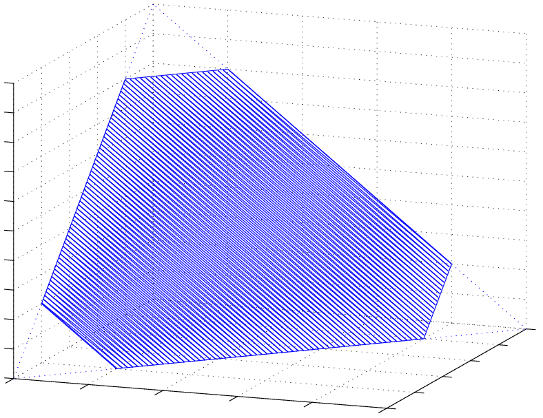
Refer to caption
Figure 3: Subset of simplex satisfying (250).

By a symmetric argument, we have

12n/2​1b​1−b2​𝐞≥𝐝¯≜12n/2​b1−b2​𝐞+𝐝≥𝟎\frac{1}{2^{n/2}}\frac{1}{b\sqrt{1-b^{2}}}\mathbf{e}\geq\bar{\mathbf{d}}\triangleq\frac{1}{2^{n/2}}\frac{b}{\sqrt{1-b^{2}}}\mathbf{e}+\mathbf{d}\geq\mathbf{0} (252)

Since 𝐜¯≜12n/2​a1−a2​𝐞+𝐜\bar{\mathbf{c}}\triangleq\frac{1}{2^{n/2}}\frac{a}{\sqrt{1-a^{2}}}\mathbf{e}+\mathbf{c} and 𝐝¯≜12n/2​b1−b2​𝐞+𝐝\bar{\mathbf{d}}\triangleq\frac{1}{2^{n/2}}\frac{b}{\sqrt{1-b^{2}}}\mathbf{e}+\mathbf{d},

𝐜¯T​𝐝¯=\displaystyle\bar{\mathbf{c}}^{T}\bar{\mathbf{d}}= (12n/2​a1−a2​𝐞+𝐜)T​(12n/2​b1−b2​𝐞+𝐝)\displaystyle\left(\frac{1}{2^{n/2}}\frac{a}{\sqrt{1-a^{2}}}\mathbf{e}+\mathbf{c}\right)^{T}\left(\frac{1}{2^{n/2}}\frac{b}{\sqrt{1-b^{2}}}\mathbf{e}+\mathbf{d}\right)
=\displaystyle= a​b(1−a2)​(1−b2)+12n/2​a1−a2​𝐞T​𝐝+12n/2​b1−b2​𝐞T​𝐜+𝐜T​𝐝\displaystyle\frac{ab}{\sqrt{(1-a^{2})(1-b^{2})}}+\frac{1}{2^{n/2}}\frac{a}{\sqrt{1-a^{2}}}\mathbf{e}^{T}\mathbf{d}+\frac{1}{2^{n/2}}\frac{b}{\sqrt{1-b^{2}}}\mathbf{e}^{T}\mathbf{c}+\mathbf{c}^{T}\mathbf{d}
=\displaystyle= a​b(1−a2)​(1−b2)+𝐜T​𝐝\displaystyle\frac{ab}{\sqrt{(1-a^{2})(1-b^{2})}}+\mathbf{c}^{T}\mathbf{d} (253)

Then,

max𝐜,𝐝𝐜T​𝐝=max𝐜¯,𝐝¯𝐜¯T​𝐝¯−a​b(1−a2)​(1−b2)\max_{\mathbf{c},\mathbf{d}}\quad\mathbf{c}^{T}\mathbf{d}=\max_{\bar{\mathbf{c}},\bar{\mathbf{d}}}\quad\bar{\mathbf{c}}^{T}\bar{\mathbf{d}}-\frac{ab}{\sqrt{(1-a^{2})(1-b^{2})}} (254)

The feasible sets of 𝐜¯\bar{\mathbf{c}} and 𝐝¯\bar{\mathbf{d}} are defined as follows,

𝒞≜\displaystyle\mathcal{C}\triangleq {𝐱:12n/21a​1−a2𝐞≥𝐱≥𝟎and𝐞T𝐱=2n/2a1−a2}\displaystyle\left\{\mathbf{x}:\frac{1}{2^{n/2}}\frac{1}{a\sqrt{1-a^{2}}}\mathbf{e}\geq\mathbf{x}\geq\mathbf{0}\quad\text{and}\quad\mathbf{e}^{T}\mathbf{x}=2^{n/2}\frac{a}{\sqrt{1-a^{2}}}\right\} (255)
𝒟≜\displaystyle\mathcal{D}\triangleq {𝐱:12n/21b​1−b2𝐞≥𝐱≥𝟎and𝐞T𝐱=2n/2b1−b2}\displaystyle\left\{\mathbf{x}:\frac{1}{2^{n/2}}\frac{1}{b\sqrt{1-b^{2}}}\mathbf{e}\geq\mathbf{x}\geq\mathbf{0}\quad\text{and}\quad\mathbf{e}^{T}\mathbf{x}=2^{n/2}\frac{b}{\sqrt{1-b^{2}}}\right\} (256)

Consider the following optimization problem

max𝐜¯∈𝒞,𝐝¯∈𝒟𝐜¯T​𝐝¯\max_{\bar{\mathbf{c}}\in\mathcal{C},\bar{\mathbf{d}}\in\mathcal{D}}\quad\bar{\mathbf{c}}^{T}\bar{\mathbf{d}} (257)

In the following, we will show that there exist 𝒞′⊆𝒞\mathcal{C}^{\prime}\subseteq\mathcal{C} and 𝒟′⊆𝒟\mathcal{D}^{\prime}\subseteq\mathcal{D} such that

max𝐜¯∈𝒞,𝐝¯∈𝒟𝐜¯T​𝐝¯=max𝐜¯∈𝒞′,𝐝¯∈𝒟′𝐜¯T​𝐝¯\max_{\bar{\mathbf{c}}\in\mathcal{C},\bar{\mathbf{d}}\in\mathcal{D}}\quad\bar{\mathbf{c}}^{T}\bar{\mathbf{d}}=\max_{\bar{\mathbf{c}}\in\mathcal{C}^{\prime},\bar{\mathbf{d}}\in\mathcal{D}^{\prime}}\quad\bar{\mathbf{c}}^{T}\bar{\mathbf{d}} (258)

If we assume that

max𝐜¯∈𝒞𝐜¯T​𝐝¯\displaystyle\max_{\bar{\mathbf{c}}\in\mathcal{C}}\quad\bar{\mathbf{c}}^{T}\bar{\mathbf{d}} =max𝐜¯∈𝒞′𝐜¯T𝐝¯∀𝐝¯∈𝒟\displaystyle=\max_{\bar{\mathbf{c}}\in\mathcal{C}^{\prime}}\quad\bar{\mathbf{c}}^{T}\bar{\mathbf{d}}\qquad\forall\bar{\mathbf{d}}\in\mathcal{D} (259)
max𝐝¯∈𝒟𝐜¯T​𝐝¯\displaystyle\max_{\bar{\mathbf{d}}\in\mathcal{D}}\quad\bar{\mathbf{c}}^{T}\bar{\mathbf{d}} =max𝐝¯∈𝒟′𝐜¯T𝐝¯∀𝐜¯∈𝒞\displaystyle=\max_{\bar{\mathbf{d}}\in\mathcal{D}^{\prime}}\quad\bar{\mathbf{c}}^{T}\bar{\mathbf{d}}\qquad\forall\bar{\mathbf{c}}\in\mathcal{C} (260)

and we also assume that the set 𝒞′\mathcal{C}^{\prime} (𝒟′\mathcal{D}^{\prime} respectively) does not depend on the value of 𝐝¯\bar{\mathbf{d}} (𝐜¯\bar{\mathbf{c}}), then we have

max𝐜¯∈𝒞,𝐝¯∈𝒟𝐜¯T​𝐝¯\displaystyle\max_{\bar{\mathbf{c}}\in\mathcal{C},\bar{\mathbf{d}}\in\mathcal{D}}\quad\bar{\mathbf{c}}^{T}\bar{\mathbf{d}} =max𝐜¯∈𝒞max𝐝¯∈𝒟𝐜¯T𝐝¯\displaystyle=\max_{\bar{\mathbf{c}}\in\mathcal{C}}\quad\max_{\bar{\mathbf{d}}\in\mathcal{D}}\quad\bar{\mathbf{c}}^{T}\bar{\mathbf{d}}
=1​max𝐜¯∈𝒞max𝐝¯∈𝒟′𝐜¯T​𝐝¯\displaystyle\overset{1}{=}\max_{\bar{\mathbf{c}}\in\mathcal{C}}\quad\max_{\bar{\mathbf{d}}\in\mathcal{D}^{\prime}}\quad\bar{\mathbf{c}}^{T}\bar{\mathbf{d}}
=2​max𝐝¯∈𝒟′max𝐜¯∈𝒞𝐜¯T​𝐝¯\displaystyle\overset{2}{=}\max_{\bar{\mathbf{d}}\in\mathcal{D}^{\prime}}\quad\max_{\bar{\mathbf{c}}\in\mathcal{C}}\quad\bar{\mathbf{c}}^{T}\bar{\mathbf{d}}
=3​max𝐝¯∈𝒟′max𝐜¯∈𝒞′𝐜¯T​𝐝¯\displaystyle\overset{3}{=}\max_{\bar{\mathbf{d}}\in\mathcal{D}^{\prime}}\quad\max_{\bar{\mathbf{c}}\in\mathcal{C}^{\prime}}\quad\bar{\mathbf{c}}^{T}\bar{\mathbf{d}}
=max𝐜¯∈𝒞′,𝐝¯∈𝒟′𝐜¯T𝐝¯\displaystyle=\max_{\bar{\mathbf{c}}\in\mathcal{C}^{\prime},\bar{\mathbf{d}}\in\mathcal{D}^{\prime}}\quad\bar{\mathbf{c}}^{T}\bar{\mathbf{d}} (261)

where

  1. 1.

    because of (260);

  2. 2.

    because we assume that the set 𝒟′\mathcal{D}^{\prime} does not depend on the value of 𝐜¯\bar{\mathbf{c}};

  3. 3.

    because of (259).

Now we need to show our assumptions, (259) and (260), are valid, for which we need the following lemma.

Lemma 6

[22, p. 722] Let 𝒞\mathcal{C} be a convex subset of ℝn\mathbb{R}^{n}, and let 𝒞∗\mathcal{C}^{\ast} be the set of minima of a concave function f:𝒞⟼ℝf:\mathcal{C}\longmapsto\mathbb{R} over 𝒞\mathcal{C}. If 𝒞\mathcal{C} is closed and contains at least one extreme point, and 𝒞∗\mathcal{C}^{\ast} is nonempty, then 𝒞∗\mathcal{C}^{\ast} contains some extreme point of 𝒞\mathcal{C}.

Here the extreme point is defined as follows:

Definition 2

[22, p. 721] A vector 𝐱\mathbf{x} is said to be an extreme point of a convex set 𝒞\mathcal{C} if 𝐱\mathbf{x} belongs to 𝒞\mathcal{C} and there do not exist vectors 𝐲∈𝒞\mathbf{y}\in\mathcal{C} and 𝐳∈𝒞\mathbf{z}\in\mathcal{C}, with 𝐲≠𝐱\mathbf{y}\neq\mathbf{x} and 𝐳≠𝐱\mathbf{z}\neq\mathbf{x}, and a scalar α∈(0,1)\alpha\in(0,1) such that 𝐱=α​𝐲+(1−α)​𝐳\mathbf{x}=\alpha\mathbf{y}+(1-\alpha)\mathbf{z}. An equivalent definition is that 𝐱\mathbf{x} cannot be expressed as a convex combination of some vectors of 𝒞\mathcal{C}, all of which are different from 𝐱\mathbf{x}.

Thus, if we assume

𝒞′\displaystyle\mathcal{C}^{\prime} ≜{extreme points of ​𝒞}\displaystyle\triangleq\{\text{extreme points of }\mathcal{C}\} (262)
𝒟′\displaystyle\mathcal{D}^{\prime} ≜{extreme points of ​𝒟}\displaystyle\triangleq\{\text{extreme points of }\mathcal{D}\} (263)

(259) and (260) will be satisfied. We observe that the set 𝒞′\mathcal{C}^{\prime} (respectively, the set 𝒟′\mathcal{D}^{\prime}), which consists of all the extreme points in the set 𝒞\mathcal{C} (in the set 𝒟\mathcal{D} ), does not depend on the value of 𝐝¯\bar{\mathbf{d}} (𝐜¯\bar{\mathbf{c}}).

Next, we determine the extreme point set 𝒞′\mathcal{C}^{\prime} in the following lemma.

Lemma 7

The set 𝒞′\mathcal{C}^{\prime} consists of all the vectors, each of which contains 2n​a22^{n}a^{2} non-zero entries with value 12n/2​1a​1−a2\frac{1}{2^{n/2}}\frac{1}{a\sqrt{1-a^{2}}}, when nn is sufficiently large.

Proof:  We define the set 𝒞′′\mathcal{C}^{\prime\prime} as the set where each element contains 2n​a22^{n}a^{2} non-zero entries equal to 12n/2​1a​1−a2\frac{1}{2^{n/2}}\frac{1}{a\sqrt{1-a^{2}}}. It is easy to see that every vector in 𝒞′′\mathcal{C}^{\prime\prime} is within the set 𝒞\mathcal{C}. We need to show that any vector in the set 𝒞\mathcal{C} is a convex combination of some vectors in 𝒞′′\mathcal{C}^{\prime\prime}. This can be proven by induction. It is easy to see that, if a vector such that 2n−12^{n}-1 out of 2n2^{n} entries take values from {0,12n/2​1a​1−a2}\{0,\frac{1}{2^{n/2}}\frac{1}{a\sqrt{1-a^{2}}}\}, the last entry will converge to 00, when nn goes to infinity. Let 𝐬∈𝒞\mathbf{s}\in\mathcal{C} such that ll out of 2n2^{n} entries take values in (0,12n/2​1a​1−a2)(0,\frac{1}{2^{n/2}}\frac{1}{a\sqrt{1-a^{2}}}). Then, we choose any 22 out of these ll entries, which are equal to α\alpha and β\beta, respectively. If α+β≤12n/2​1a​1−a2\alpha+\beta\leq\frac{1}{2^{n/2}}\frac{1}{a\sqrt{1-a^{2}}}, then

[⋯α⋯β⋯]\displaystyle\begin{bmatrix}\cdots&\alpha&\cdots&\beta&\cdots\end{bmatrix}
=βα+β​[⋯0⋯α+β⋯]+αα+β​[⋯α+β⋯0⋯]\displaystyle\qquad\qquad=\frac{\beta}{\alpha+\beta}\begin{bmatrix}\cdots&0&\cdots&\alpha+\beta&\cdots\end{bmatrix}+\frac{\alpha}{\alpha+\beta}\begin{bmatrix}\cdots&\alpha+\beta&\cdots&0&\cdots\end{bmatrix} (264)

If α+β≥12n/2​1a​1−a2\alpha+\beta\geq\frac{1}{2^{n/2}}\frac{1}{a\sqrt{1-a^{2}}}, then

[⋯α⋯β⋯]\displaystyle\begin{bmatrix}\cdots&\alpha&\cdots&\beta&\cdots\end{bmatrix}
=12n/2​1a​1−a2−β22n/2​1a​1−a2−α−β​[⋯12n/2​1a​1−a2⋯α+β−12n/2​1a​1−a2⋯]\displaystyle\qquad\qquad=\frac{\frac{1}{2^{n/2}}\frac{1}{a\sqrt{1-a^{2}}}-\beta}{\frac{2}{2^{n/2}}\frac{1}{a\sqrt{1-a^{2}}}-\alpha-\beta}\begin{bmatrix}\cdots&\frac{1}{2^{n/2}}\frac{1}{a\sqrt{1-a^{2}}}&\cdots&\alpha+\beta-\frac{1}{2^{n/2}}\frac{1}{a\sqrt{1-a^{2}}}&\cdots\end{bmatrix}
+12n/2​1a​1−a2−α22n/2​1a​1−a2−α−β​[⋯α+β−12n/2​1a​1−a2⋯12n/2​1a​1−a2⋯]\displaystyle\qquad\qquad\quad\;+\frac{\frac{1}{2^{n/2}}\frac{1}{a\sqrt{1-a^{2}}}-\alpha}{\frac{2}{2^{n/2}}\frac{1}{a\sqrt{1-a^{2}}}-\alpha-\beta}\begin{bmatrix}\cdots&\alpha+\beta-\frac{1}{2^{n/2}}\frac{1}{a\sqrt{1-a^{2}}}&\cdots&\frac{1}{2^{n/2}}\frac{1}{a\sqrt{1-a^{2}}}&\cdots\end{bmatrix} (265)

which means that 𝐬\mathbf{s} can be expressed as a convex combination of two vectors. These two vectors belong to set 𝒞\mathcal{C} and both of them have l−1l-1 out of 2n2^{n} entries takes value in (0,12n/2​1a​1−a2)(0,\frac{1}{2^{n/2}}\frac{1}{a\sqrt{1-a^{2}}}). By induction, we can show that every vector in set 𝒞\mathcal{C} can be expressed as a convex combination of some vectors in 𝒞′′\mathcal{C}^{\prime\prime}. On the other hand, it is easy to see that any vector 𝐬\mathbf{s} in 𝒞′′\mathcal{C}^{\prime\prime} cannot be expressed as a convex combination of some vectors in the set 𝒞\mathcal{C} other than 𝐬\mathbf{s} itself. Thus we conclude that 𝒞′=𝒞′′\mathcal{C}^{\prime}=\mathcal{C}^{\prime\prime}.  ■\blacksquare

Similarly, the set 𝒟′\mathcal{D}^{\prime} consists all the vectors, each of which contains 2n​b22^{n}b^{2} non-zero entries with value 12n/2​1b​1−b2\frac{1}{2^{n/2}}\frac{1}{b\sqrt{1-b^{2}}}. Then,

max𝐜¯∈𝒞,𝐝¯∈𝒟𝐜¯T​𝐝¯=max𝐜¯∈𝒞′,𝐝¯∈𝒟′𝐜¯T​𝐝¯=min⁡(a2,b2)​1a​1−a2​1b​1−b2\max_{\bar{\mathbf{c}}\in\mathcal{C},\bar{\mathbf{d}}\in\mathcal{D}}\quad\bar{\mathbf{c}}^{T}\bar{\mathbf{d}}=\max_{\bar{\mathbf{c}}\in\mathcal{C}^{\prime},\bar{\mathbf{d}}\in\mathcal{D}^{\prime}}\quad\bar{\mathbf{c}}^{T}\bar{\mathbf{d}}=\min(a^{2},b^{2})\frac{1}{a\sqrt{1-a^{2}}}\frac{1}{b\sqrt{1-b^{2}}} (266)

and,

max𝐜,𝐝𝐜T​𝐝=\displaystyle\max_{\mathbf{c},\mathbf{d}}\quad\mathbf{c}^{T}\mathbf{d}= max𝐜¯∈𝒞,𝐝¯∈𝒟𝐜¯T​𝐝¯−a​b(1−a2)​(1−b2)\displaystyle\max_{\bar{\mathbf{c}}\in\mathcal{C},\bar{\mathbf{d}}\in\mathcal{D}}\quad\bar{\mathbf{c}}^{T}\bar{\mathbf{d}}-\frac{ab}{\sqrt{(1-a^{2})(1-b^{2})}}
=\displaystyle= min⁡(a2,b2)​1a​b​(1−a2)​(1−b2)−a​b(1−a2)​(1−b2)\displaystyle\min(a^{2},b^{2})\frac{1}{ab\sqrt{(1-a^{2})(1-b^{2})}}-\frac{ab}{\sqrt{(1-a^{2})(1-b^{2})}}
=\displaystyle= min⁡(a2,b2)​min⁡(1−a2,1−b2)​1a​b​(1−a2)​(1−b2)\displaystyle\min(a^{2},b^{2})\min(1-a^{2},1-b^{2})\frac{1}{ab\sqrt{(1-a^{2})(1-b^{2})}} (267)

Hence,

λ≤λ2​(P~U​V)​1+𝐜T​𝐝2≤λ2​(P~U​V)​1+min⁡(a2,b2)​min⁡(1−a2,1−b2)a​b​(1−a2)​(1−b2)2\lambda\leq\lambda_{2}(\tilde{P}_{UV})\frac{1+\mathbf{c}^{T}\mathbf{d}}{2}\leq\lambda_{2}(\tilde{P}_{UV})\frac{1+\frac{\min(a^{2},b^{2})\min(1-a^{2},1-b^{2})}{ab\sqrt{(1-a^{2})(1-b^{2})}}}{2} (268)

The lower bound of λ\lambda can be derived in a similar manner. We rewrite (B.2) in the following form

P~X1​X2\displaystyle\tilde{P}_{X_{1}X_{2}} =[a1−a2]​[b1−b2]+(−λ)​[1−a2−a]​[−1−b2b]\displaystyle=\left[\begin{array}[]{c}a\\ \sqrt{1-a^{2}}\end{array}\right]\left[\begin{array}[]{cc}b&\sqrt{1-b^{2}}\end{array}\right]+(-\lambda)\left[\begin{array}[]{c}\sqrt{1-a^{2}}\\ -a\end{array}\right]\left[\begin{array}[]{cc}-\sqrt{1-b^{2}}&b\end{array}\right]

By the same arguments as above, we obtain

−λ\displaystyle-\lambda ≤λ2​(P~U​V)​1+min⁡(1−a2,b2)​min⁡(a2,1−b2)a​b​(1−a2)​(1−b2)2\displaystyle\leq\lambda_{2}(\tilde{P}_{UV})\frac{1+\frac{\min(1-a^{2},b^{2})\min(a^{2},1-b^{2})}{ab\sqrt{(1-a^{2})(1-b^{2})}}}{2} (275)

Combining (268) and (275), we have

−λ2​(P~U​V)​1+min⁡(1−a2,b2)​min⁡(a2,1−b2)a​b​(1−a2)​(1−b2)2≤λ≤λ2​(P~U​V)​1+min⁡(a2,b2)​min⁡(1−a2,1−b2)a​b​(1−a2)​(1−b2)2-\lambda_{2}(\tilde{P}_{UV})\frac{1+\frac{\min(1-a^{2},b^{2})\min(a^{2},1-b^{2})}{ab\sqrt{(1-a^{2})(1-b^{2})}}}{2}\leq\lambda\leq\lambda_{2}(\tilde{P}_{UV})\frac{1+\frac{\min(a^{2},b^{2})\min(1-a^{2},1-b^{2})}{ab\sqrt{(1-a^{2})(1-b^{2})}}}{2} (276)

■\blacksquare

References

  • [1] W. Kang and S. Ulukus. A single-letter upper bound for the sum rate of multiple access channels with correlated sources. In Proc. 39th Asilomar Conf. on Signals, Systems and Computers, Pacific Grove, CA, Oct. 2005.
  • [2] W. Kang and S. Ulukus. An outer bound for multiple access channels with correlated sources. In Proc. 40th Conf. on Information Sciences and Systems (CISS), Princeton, NJ, Mar. 2006.
  • [3] W. Kang and S. Ulukus. An outer bound for multi-terminal rate-distortion region. In Proc. IEEE International Symp. on Information Theory (ISIT), Seattle, WA, Jul. 2006.
  • [4] S. Y. Tung. Multiterminal Source Coding. Ph.D. Dissertation, Cornell University, 1978.
  • [5] K. B. Housewright. Source Coding Studies for Multiterminal Systems. Ph.D. Dissertation, University of California, Los Angeles, 1977.
  • [6] T. Berger. Multi-terminal source coding. Chapter in The Information Theory Approach to Communications (G. Longo, ed.), Springer-Verlag, 1978.
  • [7] T. M. Cover, A El Gamal, and M. Salehi. Multiple access channel with arbitrarily correlated sources. IEEE Trans. Inform. Theory, 26:648–657, Nov. 1980.
  • [8] R. Ahlswede and T. S. Han. On source coding with side information via a multiple-access channel and related problems in multi-user information theory. IEEE Trans. Inform. Theory, 29(3):396–412, 1983.
  • [9] T. M. Cover and J. A. Thomas. Elements of Information Theory. John Wiley and Sons, 1991.
  • [10] H. S. Witsenhausen. On sequences of pairs of dependent random variables. SIAM Journal on Applied Mathematics, 28:100–113, Jan. 1975.
  • [11] K. Marton. The structure of isomorphisms of discrete memoryless correlated sources. Zeitschrift für Wahrscheinlichkeitstheorie und verwandte Gebiete, 56(3):317–327, 1981.
  • [12] A. Berman and R. J. Plemmons. Nonnegative matrices in the mathematical sciences. Academic Press, 1979.
  • [13] R. A. Horn and C. R. Johnson. Matrix Analysis. Cambridge, 1985.
  • [14] R. A. Horn and C. R. Johnson. Topics in Matrix Analysis. Cambridge, 1991.
  • [15] A. D. Wyner and J. Ziv. The rate-distortion function for source coding with side information at the decoder. IEEE Trans. Inform. Theory, 22(1):1–10, 1976.
  • [16] A. B. Wagner and V. Anantharam. An infeasibility result for the multiterminal source-coding problem. Submitted to IEEE Trans. Inform. Theory, 2006, http://arxiv.org/pdf/cs.IT/0511103.
  • [17] S. Servetto. The region of achievable rates for multiterminal source coding. Submitted to the IEEE Transactions on Information Theory, 2006, http://cn.ece.cornell.edu/publications/papers/20060228/pp1.pdf.
  • [18] G. Dueck. A note on the multiple access channel with correlated sources. IEEE Trans. Inform. Theory, 27:232–235, Mar. 1981.
  • [19] S. S. Pradhan, S. Choi, and K. Ramchandran. A graph-based framework for transmission of correlated sources over multiple access channels. Submitted to IEEE Trans. Inform. Theory, 2006, http://www.eecs.umich.edu/∼\simpradhanv/paper/ittrans06_1.pdf.
  • [20] A. Lapidoth and S. Tinguely. Sending a bi-variate Gaussian source over a Gaussian MAC. In Proc. IEEE International Symp. on Information Theory (ISIT), Seattle, WA, Jul. 2006.
  • [21] G. W. Stewart. On the early history of the singular value decomposition. SIAM Review, 35:551–566, Dec. 1993.
  • [22] D. P. Bertsekas. Nonlinear Programming. Athena Scientific, 2 edition, 1999.