A Continuum Theory for Unstructured Mesh Generation in Two Dimensions
Abstract
A continuum description of unstructured meshes in two dimensions, both for planar and curved surface domains, is proposed. The meshes described are those which, in the limit of an increasingly finer mesh (smaller cells), and away from irregular vertices, have ideally-shaped cells (squares or equilateral triangles), and can therefore be completely described by two local properties: local cell size and local edge directions. The connection between the two properties is derived by defining a Riemannian manifold whose geodesics trace the edges of the mesh. A function , proportional to the logarithm of the cell size, is shown to obey the Poisson equation, with localized charges corresponding to irregular vertices. The problem of finding a suitable manifold for a given domain is thus shown to exactly reduce to an Inverse Poisson problem on , of finding a distribution of localized charges adhering to the conditions derived for boundary alignment. Possible applications to mesh generation are discussed.
Keywords:
Unstructured mesh generation, differential geometry.1 Overview
A mesh is a partition of a domain into smaller parts, typically with simpler geometry, called cells. In two dimensions, both on the plane and on curved surfaces, cells are usually triangles or quadrilaterals. The shapes of the cells may be important; for many applications, cells with shapes similar to an equilateral triangle or a square are preferred. The problem of mesh generation can then be seen as an optimization problem: to find a partition of a domain into well-shaped cells, possibly under additional demands, such as cell size requirements.
The mesh generation problem has been the subject of extensive research. Many techniques for creating meshes exist, especially in two dimensions [1],[2],[3]. Nevertheless, some of the most popular techniques, which create good meshes in many cases, are heuristic in nature, and may create less than optimal meshes for some inputs. Two of the inherent characteristics of the mesh generation problem seem to make it very difficult to solve:
- (Characteristic 1)
-
The constraints on cells’ shapes are global. That is, the shape of one cell is constrained by the possible shapes of its neighbors, which in turn are constrained by the shapes of their neighbors, and so on. Thus, at least in principle, the constraints on the mesh layout extend over the whole domain (or more precisely, over each connected component of the domain).
- (Characteristic 2)
-
The problem combines discrete and continuous aspects. The number of cells and the mesh connectivity (i.e.: which cells are neighbors? which faces do they share?) are of discrete nature, whereas the locations of the vertices can vary continuously. These aspects are closely intertwined, preventing the sole use of purely discrete techniques (algebraic, graph-theoretic, etc.), or techniques designed for use in problems of continuous nature.

The meshes created by mesh generation algorithms can be divided into structured meshes, and unstructured meshes. A structured mesh is a mesh whose connectivity is that of a regular grid, see Fig. 1 ,(iii). By assuming the connectivity of the mesh beforehand, the problem of creating such a mesh is considerably simplified (see Characteristic 2 above), and reduces to the problem of assigning locations to the mesh vertices. One way of doing that is by finding a mapping function that maps the domain of the regular grid to the domain to be meshed, and using it to map the vertices. Such techniques are known as mapping techniques. For small enough cells, the differential properties of the mapping function at the cell’s location dictate its shape. If, for example, a mapping is angle preserving, then the inner angle of a small enough cell will be approximately preserved under the mapping. For a survey, see Ref. 2. Mapping techniques have also been offered for unstructured meshes, (in the context of smoothing a given mesh see [5],[6] and references therein), as long as the connectivity of the mesh is given beforehand.
Just as a structured mesh can be imagined as created by mapping of a region of the plane to the domain to be mapped, an unstructured mesh in two dimensions can be imagined as a surface, that is mapped onto the domain to be meshed. The simplest example is that of an unstructured mesh with just one irregular vertex (a vertex that has more or less than four cells incident upon it). The surface to be mapped in this case is a cone. This can be visualized using the Volterra construction [7]: Consider a piece of paper with an angular section cut out, see Fig. 2,(i). If the two edges of the section are identified, i.e. glued together, the paper will assume the shape of a cone, see Fig. 2,(ii). If the cone is then mapped to the plane, a regular grid drawn on the cone would be mapped to an unstructured mesh such as the one shown in Fig. 2,(iii). The mapping shown in Fig. 2,(iii) has the special property of being conformal: a small square on the cone is approximately mapped to a square on plane. This creates well shaped cells in the resulting mesh: in the limit of an increasingly smaller cell, its square shape is preserved under the conformal mapping. A similar construction can be imagined for creating an unstructured mesh with more than one irregular vertex; each irregular vertex will then correspond to one “cone tip” of the surface.
The approach of the present work to the problem of creating unstructured meshes can be expressed as follows: given a domain to be meshed, what surface, with a square grid drawn upon it, can be mapped conformally into this domain? Thus, it is not just the mapping function that is sought after, but rather the surface to be mapped together with the mapping function. Unlike mapping techniques, however, the mapping function is required to be conformal.

A mathematical framework highly suitable for dealing with such questions is Riemannian geometry. Given the domain to be meshed, Riemannian geometry allows one to define a “new geometry” for that domain. This includes a redefinition of the distances between points of the domain, and it is used here to redefine distances such that a cell edge have unit length. Thus, instead of defining the surface that is mapped and the mapping function separately, both are treated together, as the mapping induces a new distance definition on the domain to be meshed. For example, the cone in Fig. 2,(ii) and the surface in Fig. 2 ,(iii) have the “same geometry” (i.e. are isometric) if the distances in Fig. 2,(iii) are defined such that cell-edges have unit length. Using the terminology of Riemannian geometry, the problem can be restated as assigning a new metric to the domain being meshed, having the following properties:
- (Property 1)
-
The metric is locally flat everywhere, except at some points, called cone points. A “flat” region can be imagined as a bent, but not stretched, piece of paper. The cone points are the “tips of the cones” as described above.
- (Property 2)
-
A single real function is defined in the domain (except at cone points), such that at any given point , the new metric at is proportional to the original metric : , with ,. (On the plane with Cartesian coordinates .) We stress that the proportionality can vary throughout the domain. The quantity is the local change in the distance definition and will be associated with the local cell size. (In manifold theory terminology, the metric is conformally related to ).
These two properties are not sufficient for our purposes. First of all, as the Volterra construction implies, for a grid of squares to be drawn around a cone tip, the total angle as measured around the tip must be a multiple of radians. Secondly, the mesh must be aligned along the boundary, see Fig. 3. To formalize these demands, we define the direction of mesh-edges at each point on the surface. Since the edges are assumed to form right angles at incidence, this direction is defined up to an addition of radians11 1 In the case of a triangular mesh, the direction will be defined up to an addition of .. The four directions at each point will hence be called a cross, and the field of directions on the entire domain being meshed will be called a cross-field. The cross-field is related to the new metric by requiring that the curves, generated by following the directions of the cross-field, along which the edges will be laid, will be geodesics of the new metric . (Geodesics are the generalizations of straight lines for surfaces and manifolds.) The boundary alignment is formalized by requiring that the crosses be aligned with the boundary.
We therefore add the following property to the required properties of the new metric:
- (Property 3)
-
A cross-field exists. (Exact definition is given in section 3.)
Property 1 states that the Gaussian curvature of the manifold with metric be identically zero everywhere, except at cone points. Combined with the equation of Property 2, the two formulas give a remarkably simple result, viz. that must obey the Poisson equation everywhere exept at cone points, where is the Gaussian curvature of the surface. This is a well known result in conformal geometry, see section 3.

The main result of the present work is that for a cross-field to exist the function , which uniquely defines the manifold, has to obey the Poisson equation , with the Gaussian curvature of the surface to be meshed ( vanishes for the plane), and a sum of “localized charges” (Dirac delta functions). The charges are placed at the cone points’ locations, thus corresponding to the irregular vertices of the mesh. The charge strength is equal to the cone excess angle (the difference between the cone angle and ) which corresponds to the number of cells incident on the irregular vertex. For example, in the manifold shown in Fig. 2,(iii), the cone point has an excess angle of . The charge of the cone point, located at a point , corresponding to such a excess angle is , where is the Dirac delta function in two dimensions. This is the charge of any singularity corresponding to an irregular vertex surrounded by three cells. Along with the boundary alignment conditions on , the problem of finding an appropriate manifold is thus reduced to an Inverse Poisson problem, of finding a charge distribution adhering to these conditions. The reduction gives exact, global relations that the function must obey.
The inverse Poisson problem on planar domains is of interest in many fields of science and engineering (see references in section 7.3); the relevance of existing techniques to the present application remains to be examined. Another possible application is to the problem of creating a surface mesh aligned with predefined directions, which has recently attracted much attention [4],[8],[13],[14]. The algorithm described in [13] creates conformal parametrizations and meshes approximately aligned with predefined directions. In that work, the local size and the local direction are treated as independent variables. In order to reduce the number of singularities, a preprocessing step that modifies the cell size demand (the “curl correction” process) can be applied. In contrast, the theory developed in the present work uses conformality to a-priory link the cell-size and cell-direction fields, leaving just one field to work with, either the cell-size or the cell-direction. The applications of this theory to surface parameterization and surface quadrangulation problems are an interesting subject for future work.
Conformal parametrization of manifolds with conical singularities have been used in surface parametrization problems. For reviews and related work, see [9]-[13]. Mesh generation with boundaries and surface parametrization are different problems, because of the boundary alignment requirement in mesh generation. For example, the parametrization problem for planar domains is trivial: the coordinates of the plane form a good parametrization, but do not solve the mesh generation problem.
The rest of the article is organized as follows: In section 2 some elements of differential geometry are shortly reviewed. In section 3 the cross-field and -manifold are defined. Section 4 discusses the relation of the definitions in previous sections to mesh generation. Cone points are analyzed in section 5. The necessary and sufficient conditions for cross-field existence are developed in section 6. The set of conditions derived in sections 5,6 forms the core result of the work. In section 7 the theory is discussed through four case studies. Case Studies A,B are used to discuss the meaning of the conditions derived before. In Case Study C the possible structure of a mesh generation algorithm is discussed. An example quadrilateral mesh problem, though admittedly simple and artificial, demonstrates how, given an input, a manifold with cone points is constructed, adhering to the imposed conditions. This manifold allows the construction of meshes with irregular vertices; at any given point in the domain that is not an irregular vertex, at the limit of increasingly finer meshes, the cells’ shapes tend to a square. Case study D gives an example of a curved surface meshing problem, and how it is solved.
2 Parallel Transport and Geodesics
In this section basic facts from differential geometry, required in subsequent sections, are shortly reviewed. More complete accounts can be found in any textbook on differential geometry, such as [15],[16].
For a surface embedded in three-dimensional space, distances and angles on the surface can be defined by the embedding. In some coordinate system, denote by the metric given by the embedding. For example, on the plane with Cartesian coordinates, , the Kronecker delta. Another metric, , is said to be conformally related to , if there exists a real function on the surface such that
| (1) |
Given two vectors defined at some point on a surface or Riemannian manifold, the angle between them is given by
| (2) |
where summation over repeated indices (the Einstein convension) is assumed. The angle as measured with the metric is
| (3) |
Substituting in Eq. (3 ), and comparing with Eq. (2) it is found that , so the measurement of angles using the two conformally related metrics agrees.
Given a vector field on the plane (with the Euclidean metric) the question of whether two vectors at two different points are parallel has a definite answer. This is not the case on curved surfaces, and more generally, for Riemannian manifolds. There, the definition of parallel vectors at different locations generally depends on the path chosen between the points. For a curve connecting points and , the parallel transport of a vector from to along can be defined. If is such a vector at we denote its parallel translate to along by , see Fig. 4.

The geodesic curvature of a curve is the amount by which a curve “turns”. On the plane (with the Euclidean metric) turning is measured by the change of the angle of the tangent vector to the curve. On a surface (and, more generally, on a Riemannian manifold) the angle is defined relative to a vector that is parallel translated along the very same curve. For a curve , denote the tangent vector at by . Define . Then
| (4) |
where is the length parameterization of , see Fig. 5.

The parallel transport depends on the metric, so a curve can have different geodesic curvatures under different metrics. Let be the geodesic curvatures of a curve at some point , with the metrics respectively, related as in Eq. (1). (Henceforth, all quantities relating to the metric will be marked with a tilde.) Then are related by
| (5) |
where is the derivative of along the normal vector , which is defined such that form a right hand system. Eq. (5) is derived in appendix A.
A geodesic is a generalization of a straight line. It is the curve whose geodesic curvature vanishes. The equation for a geodesic of the metric is found by substituting in Eq. (5):
| (6) |
Two integral theorems are used throughout the paper. The first is the Gauss-Bonnet theorem, which relates the change in a vector undergoing parallel transport along a closed loop, to the total Gaussian curvature inside the loop. Let be a closed curve, , enclosing a region . The junction angles, , measure the change in direction of the tangent at junction points. As a convention we assume that is traversed in a counter-clockwise direction. let be a vector at . Then the angle is equal to
| (7) |
where is the Gaussian curvature.
The second integral theorem is Green’s theorem, also known as the divergence theorem, or Gauss’ theorem. Suppose is a curve enclosing a region , transversed in a counter-clockwise manner, and a function defined on the surface. Then
| (8) |
The (unconventional) minus sign appears because the normal direction to was defined such that form a right hand system, so points inwards. For a surface the Laplacian operator denotes the Laplace-Beltrami operator [16].
If two metrics are conformally related as in Eq. (1 ), and the manifold with the metric is flat, i.e.
| (9) |
a differential equation for can be derived. This can be done using the expression for the curvature in terms of . It is derived here in a different way, using the integral theorems quoted above, as this technique is used again in subsequent sections.
Suppose that a region equipped with the metric is flat, i.e. Eq. (9) holds in . Then according to the Gauss-Bonnet theorem, Eq. (7),
| (10) |
The length element for the two metrics discussed are related by
| (11) |
Substitute Eq. (5),(11) in Eq. (10) to get
| (12) |
Here Green’s theorem, Eq. (8), was used. Subtracting Eq. (10) from (12),
| (13) |
where Gauss-Bonnet was used. Since this result is true for an arbitrary flat region , the integrand must vanish, i.e., for any point in where Eq. (9) holds:
| (14) |
Eq. (14) is a differential equation for . It is a well-known result in conformal geometry, see e.g. [17],[18].
3 Cross-field and -manifold definitions
The input to the mesh generation problem is assumed to be a surface embedded in three dimensional Euclidean space, such that:
- (i)
-
Its boundary is a union of a finite number of connected components .
- (ii)
-
Every component is a piecewise closed curve.
The points where a boundary component is not differentiable will be called junction points. The set of all junction points will be denoted by .
The edges of the final mesh are to be laid along geodesic curves of a manifold that will be defined below, the -manifold. To create a high quality mesh, these curves should cross each other, and reach the boundary, at certain angles. In the case of a quadrilateral mesh, a cell with right inner angles is preferred for many applications. In the case of a triangular mesh, the preferred inner angle is radians. It is therefore natural to define the direction of edges at a point to within an addition of radians in the quadrilateral case, and radians in the triangular case. This difference between the two cases leads to slightly different results; for clarity of presentation, the quadrilateral case is presented first, and the results for the triangular case are defered to Appendix B.
The directions of edges at a point will be called a cross. The field of edge directions will be called a cross-field.
Definition 1 (Cross)
First, define an equivalence of vectors in : for 2 vectors , if and only if , are parallel or perpendicular. A cross is an element of .
Thus, a given cross is a set of vectors, every pair of which are either perpendicular or parallel.
If two vectors, defined at some point, undergo parallel transport along the same curve, the angle between two vectors is preserved: the angle before the parallel transport is equal to the angle after the parallel transport [15]. Therefore, the cross equivalence class structure is preserved, and the parallel transport of crosses is well-defined.
Let be a finite set of points in . Denote the metric on by . Supoose a metric is defined on . The following definition of a cross-field assures that the flow lines of the cross-field are geodesics, and that the crosses on the boundary are aligned with boundary.
Definition 2 (Cross-field)
A cross-field on a given manifold with metric is a mapping such that:
- (i)
-
For points , the parallel transport under the metric of to along a curve is independent of , and is equal to : .
- (ii)
-
For , the tangent belongs to the cross there: .

The flow-lines curves of a cross-field are geodesics of the metric . That is, a geodesic aligned with the cross-field at one point (i.e., whose tangent belongs to the cross at that point), is aligned with the cross-field everywhere else on the curve. This is because both the cross-field and the tangent to a geodesic are parallel-translated along the geodesic, see definition 2,(i), and the discussion preceding Eq. (6). Geodesic curves aligned with the cross-field will be called cross-field geodesics. Cross-field geodesics and their relation to the cross-field are illustrated in Fig. 6.
As before, let be a finite set of points in . We now define the -manifold.
Definition 3 (-manifold)
A -manifold is a Riemannian manifold defined on , with metric such that:
- (i)
-
is conformally related to , i.e. where is a real function on .
- (ii)
-
The -manifold is locally flat, i.e. its Gaussian curvature tensor for all points in .
- (iii)
-
For every boundary point , , the limits and exist and are continuous along at .
- (iv)
-
A cross-field with the metric exists.
The points in will be called cone points. This name is justified in section 5, see also section 1. For now, the points in are just points where is undefined.
In the following sections, the requirement that a -manifold exists is translated into conditions on the function .
4 Relation to mesh generation
The cross-field formulates the demand that mesh cells have certain inner angles. In order to have square-like shapes, the cells should further have edges of similar lengths. This is where the conformal metric property of the -manifold comes into play.
Integrating over Eq. (11), the length of a curve on a -manifold is given by
| (15) |
The area of a region of a manifold is given by [15],[16]
| (16) |
where . The tilde denotes, as before, a quantity with respect to -manifold metric .
The following claim is a consequence of the isometry of a flat manifold to the Euclidean plane [16]. It is the “manifold version” of the properties of a rectangle.
Claim 1
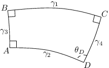
Let be 4 geodesic segments in a flat region of a manifold, organized as in Fig. 7. Suppose that the inner angles at the vertices are right angles, and is the manifold-length of the i-th side of the “rectangle”. Then the inner angle at , , is a right angle, and . The area of the “rectangle” is .
On an Euclidean plane, the properties of a rectangle allow one to lay a grid on a region of the plane. A grid can be regarded as two families of mutually perpendicular straight lines, with equal spacing between lines of each family. The same can be done for a -manifold using the “rectangle” properties stated in claim 1, see Fig. 8. The grid divides the space into square-like regions, each bounded by four geodesic segments of manifold length , that will be called manifold-edges. The regions enclosed by the manifold-edges will be called manifold-cells.

is a single, fixed number for the mesh. The overall size on the surface or plane of the manifold-cells can be controlled by adding a constant to , so the freedom in choosing is redundant, and we set . According to Claim 1 such a cell has unit -manifold area. According to Eq. (15), for small enough manifold cells (large enough ), a manifold edge of length has length , and is interpreted as the local edge length, or local cell size.
A geometrical interpretation of the relation, Eq. (6), can now be given. For a mesh with approximately square cells, the curving of manifold-edges is related to the changes in cell size in the perpendicular direction, see Fig. 9. This is quantified in Eq. (6): is the curvature of the lines defining the edges, and is the change in , which is related to local cell size by .

5 Cone-points
The existence of a cross-field restricts the possible behavior of in the vicinity of cone points. Let be a cone point, and a point that is not a cone point. Let be a simple closed curve starting from that encloses , and only of , see Fig. 10. The junction angles of are denoted by . According to cross-field definition, the cross is parallel translated to along , that is, a vector is parallel translated along , to . By the defintion of a cross, are either parallel or perpendicular, and the angle is , . Using Eq. (5),(7):
| (17) |
where is the region enclosed by .

On a -manifold a manifold-cell has unit area, so in order to have a finite number of cells, the the area of the -manifold must be finite. This will further restrict the type of singularity allowed at a point , as is now shown.
For a cone point on the surface let be a neighborhood of in which there exist isothermal coordinates . In such coordinates, which can always be found locally22 2 The original proof, due to Gauss, requires that the surface is analytic [16]. There are proofs with weaker assumptions, but these distinctions are immaterial for the present purposes., the metric takes the form: , where is a real function of . Note that on the plane, the standard Cartesian coordinates satisfy , and hence are isothermal. In isothermal coordinates the Laplace-Beltrami operator can be written as33 3 This can be seen by substituting the form of the metric tensor in isothermal coordinates into the definition of the Laplace-Beltrami operator: , see e.g. [16].
| (18) |
Eq. 18 can be seen as a generalization of the usual planar Laplacian, given by . Let be a disk of radius in , i.e. the region for which . In isothermal coordinates Eq. (14) reads
in the punctured disk . In polar isothermal coordinates , (that is, the polar coordinates corresponding to ), the general form of this solution can be written as (see e.g. [20]):
| (19) |
where is a solution to the Poisson equation in (including ), and are all real numbers.
Let be a curve tracing the circle , in the counter-clockwise direction. For given by Eq. (19), the flux of through is
| (20) |
where Green’s theorem, Eq. (8) was used to convert the first term to a surface integral. In the limit Eq. (20) becomes: , and Eq. (17) with becomes: for some . Comparing the two limiting values for we find
| (21) |
for some .
The quantity will be called the charge of the cone-point. Eq. (21) states that the charges must be multiples of .
In order to have a finite number of unit-area manifold cells, the manifold-area of a neighbourhood of must be finite. The manifold area of the disc of radius around is obtained by substituting Eq. (19) into Eq. (16):
| (22) |
Since a solution of is bounded in a compact region, does not effect the convergence of the integral, nor does , which is bounded away from zero. To converge, it is required that for every , and that . This restricts to the form
| (23) |
with . This is a solution of the Poisson equation for one point-source
| (24) |
in a neighborhood of . For many cone points Eq.
(24) becomes:
Condition 1:
obeys the equation
| (25) |
the Poisson equation with point sources (delta functions) , with , .

For a planar domain, Condition 1 can be rewritten as
Condition 1 (planar domain):
For , can be written as
with , , and on .
Fig. 11 shows selected cross-field geodesics for a planar domain around a singularity (with ), spaced at manifold-distances of from each other, for different singularity strengths. In practice, good candidates for meshes will only have singularities of charge , due to the inner-angles of cells incident on the singularity, see also Remark 7 in section 7.3 below.
To summarize this section, it has been shown that the existence of a grid of geodesics that follow a cross-field and create a finite number of cells, restrict the form that the function can take. This is formulated in Condition 1, stating that must obey the Poisson equation, with delta function charges corresponding to cone points.
6 Boundary Alignment Conditions
This section examines the conditions for boundary alignment of a cross-field, see Definition 2,(ii). Three conditions will shown to be necessary. Sufficiency of the conditions is discussed in section 6.1.
We start by developing an equation that will be used in the derivation of the conditions below. Let be two points on two boundary curves , respectively. Note that may be the same boundary curve: . Let be some curve from to , see Fig. 12. For denote by . By definition of a cross-field, the cross in must be parallel-translated along to the cross in . The cross in contains , and the cross in contains so
| (26) |

where is defined as
| (27) |
The last equality is due to the preservation of angle in parallel transport, together with Eq. (4). Eq. (5) and (11) can now be used with Eq. (27)
Substituting this into Eq. (26) we find the relation
| (28) |
Eq. (28) is used below to develop the next three conditions.

Let be a segment of a boundary curve , between points that are not junction points: , and suppose does not contain junction points. Choose some smooth curve from to , whose tangents at coincide with the tangents to , see Fig. 13, i.e. , and such that the region enclosed by does not include any cone points. According to Eq. (28),
| (29) |
According to Gauss-Bonnet, Eq. (7),
| (30) |
where is the area enclosed by . Green’s theorem gives
| (31) |
Substituting Eq. (30),(31) and recalling that in (see Eq. (14)), Eq. (29) now reads
| (32) |
When , the integrals both tend to zero, and the equality is possible only if . Then
| (33) |
and with it follows that
Condition 2:
For a point with boundary curvature , must satisfy
The equation in Condition 2 is the same as Eq. (6). This is not incidental: Condition 2 causes cross-field geodesics, that are close and parallel to the boundary, to follow the shape of the boundary, as shown in Fig. 3.
For a point , that is, a junction or cone point of the boundary, let be two points on both sides of the junction point , and the boundary segment from to , see Fig. 14. Let be a curve from to . The Gauss-Bonnet theorem, Eq. (7), for the curve reads
| (34) |
where is inner angle at , and are defined as in Eq. (28). Eq. (28) reads

Condition 3:
For a curve as described above:
| (36) |
with . This requires to have a singularity at . On the plane, for example, has a singularity of type at distance from .
The final condition to be imposed on is a relation between different boundary components, and accordingly, its formulation is not local. It is just a restatment of Eq. (28).
Condition 4:
For two boundary components , and a curve connecting to it is necessary that
| (37) |
for an integer . are defined as in Eq. (28).
Condition 4 states that the total flux through a curve connecting the two boundary components can only belong to a certain, discrete, set of values.

Condition 4 has can be put in a simpler form when the domain is planar. Let be the angle between the -axis and , see Fig. 15. Then, because is equal to the change from to in the angle between the tangent to and the -axis we have
Condition 4 for the planar case then reads
Condition 4 (planar domain):
For two boundary components , and a curve connecting to it is necessary that
for an integer .
6.1 Sufficiency of the conditions
In the previous sections Conditions 1-4 were shown to be necessary for the existance of a -manifold. This section considers the question: when are Conditions 1-4 sufficient? It turns out that the answer to this question depends on the genus of the surface. Intuitively, the genus of a surface is the number of handles a surface has [22]. For example a sphere or a disk are genus-0 surfaces, and a torus is a genus-1 surface. A surface of any genus can have any number of boundaries: for example, any planar domain, with an arbitrary number of boundaries, is a genus-0 surface.
The following theorem states that for genus zero surfaces, Conditions 1-4 are sufficient. The theorem also shows how to construct the cross-field given the function . For higher genus surfaces, an additional condition is required, constraining the parallel transport along curves “passing through” the handles of higher genus surfaces. A detailed disscusion is out of the scope of the present work, but a brief account is given in Appendix C.
Theorem 4
Suppose is a surface of genus-. Let be some boundary point such that . Assume satisfies Conditions (1),(2),(3), and satisfies Condition (4) with curves between and points , for every . Let be the (unique) cross such that . For every , let be some curve from to , and define to be the translate of along . Then is independent of , and is a cross-field.
The proof is given in Appendix C.
Remark 5
If the surface is closed, i.e. has no boundaries, the cross at some point on the surface must be fixed for the cross-field to be unique.
7 Discussion: Finding a -manifold
According to Theorem 4 in section 6.1, if a function is found, satisfying Conditions 1-4, a -manifold exists, and its cross-field can be calculated.
In addition to Conditions 1-4, a meshing problem can include other requirements, such as cell size requirements on the boundaries, or inside the mesh. Clearly, finding an appropriate -manifold then depends on these conditions as well. In what follows the problem of finding a -manifold under different requirements will be discussed.
The next three sections focus on the planar case, and give concrete examples of the theory presented above. The fourth section gives an example of a curved surface meshing, that is solved analytically.
After finding a valid -manifold, the final stage of a mesh generation process involves finding a discrete partition into well-shaped manifold cells, see below. A comprehensive discussion of this step will not be given here, but some comments on this process will be made as part of the case studies.
7.1 Case Study A: No singularities are needed
Sections 7.1,7.2,7.3 deal with meshing of planar domains. On the plane, the geodesic curvature reduces to the curvature of a planar curve, which will be denoted by .
We start with a simple planar case. Suppose that the boundary has only one connectivity element (loop) . Furthermore, suppose that all junction angles (equal to , the inner angle) are multiples of , and that the their sum is . In such a case, Condition 4 is empty (since there is only one boundary loop), and Condition 3 can be satisfied with , and without any additional singularities at the junction points. Condition 2 are Neumann boundary conditions on . is a simple loop, and the sum of junction angles is , thus the total is flux of through the boundary is
Therefore given the boundary conditions a solution to the Laplace equation (that is, with no singularities) exists, and is unique up to an additive constant [19].
A simple example of such a case, that can be solved analytically, is a section of an annulus between two radial lines, see Fig. 16. The boundary conditions on the sides of the boundary, dictated by the shape of the boundary are given, according to Condition 2, by (note that can be negative, see Eq. (4)):
| (38) | ||||


The solution to the Laplace equation with boundary conditions given in Eq. (38) is
| (39) |
Here, is the distance from the center of the ring, and is a constant. Note that no specification of the local cell size was given in the input, and, according to section 4, the resulting local cell-size function is part of the solution. It is given by , with .
Fig. 17 shows geodesics starting from the boundaries. To create the figure, as well as Fig. (18), Fig. (19) and Fig. (20 ),(iii), the Poisson equation was solved numerically on a triangular mesh inside the domain (even though an analytical solution is known in the case shown in Fig. (17)). The geodesics were calculated by solving the geodesic equation, Eq. (6), with initial tangent perpendicular to the boundary. The integration constant was chosen such that 10 manifold-edges will fit on the radial boundaries, i.e. that . This fixes the solution completely, and gives a non-integer manifold-length along the arcs. Fig. 17,(i) shows geodesics spaced at unit manifold-distances of each other. Whereas the radial direction fits exactly 10 manifold-edges of equal length, the manifold-distance from the left-most geodesic to the boundary is less then 1, resulting in manifold cells with high aspect ratio in the left-most row of cells. In Fig. 17, (ii), two different spacings are used, so as to allow equal spacing in both the radial and tangential directions, with an aspect ratio as close to one as possible. Fig. 18 shows an example with a more elaborate boundary adhering to the restrictions stated in the beginning of section 7.1. Again, the equally-spaced geodesics of Fig. 18,(ii) do not form well-shaped (or even valid) cells44 4 The geodesics shown near the right and bottom of the intrusion in Fig. 18 are not parallel to the boundary. This is due to the change in cell size. Other geodesics, closer to the boundary, follow the shape of the boundary more closely.. A valid discretization can be created, e.g. by using geodesics emanating from the junction points to decompose the domain.
Remark 6
Note that in general, local edge directions are not aligned with the flow lines of , as can be seen e.g in Fig. 18.

We now lift the restriction that all junction angles are multiples of . If the angle is not , Condition 3 requires that have a radial-singularity at the junction point. Denote the junction inner-angle by . Suppose that contains a singularity caused by placing a charge at the junction point, i.e. . (If two or more boundary segments are incident on the same point, other functions may be required.) Let be the curve formed by traversing an arc of the circle at a distance from the junction point in a counter-clockwise direction, as in Fig. 14. Then according to Condition 3 (Eq. (36))
for , so
| (40) |
for . must be positive, since otherwise , causing the manifold-area to diverge at the singularity, by the same argument as presented in section 5. Apart from this restriction the number is not fixed, and affects the manifold-angle at the singularity, i.e. the number of manifold-cells incident on the junction.

The example in Fig. 19 shows a domain enclosed by one boundary element. In one junction, the inner angle is , which, according to Eq. (40), requires a singularity of charge , for placed at the junction. The solution was calculated by decomposing into 2 contributions: . is the charge potential, . was computed by numerically solving the Laplace equation on a triangular mesh with boundary conditions .
The examples that were presented in this case study could have been obtained by a conformal mapping from a “logical” domain. This is, of course, not true when cone points are present inside the domain55 5 Even without cone-points inside the domain, this is not always possible, since the mapping from to the “logical” domain is not, in general, one-to-one. In manifold-theory terminology, even if the manifold is flat and simply connected, it is not necessarily covered by a single geodesic coordinate patch of the conformal metric..
Note, however, that unlike many mapping techniques, even if such a “logical” domain can be defined, its shape is not fixed in advance, and is part of the solution. This is even more pronounced in problems involving cone points, see below. Conformal mappings that are also boundary aligned are quite limited in the scope of problems they can mesh, and sometimes yield large differences in cell size (as in the example shown in Fig. 18). That is why in mapping techniques the conformal restriction is lifted, see e.g. Ref. 2. In the present work, the conformal condition (in its manifold formulation) is retained, and instead cone points are allowed into the manifold.
7.2 Case Study B: Two boundaries, no boundary cell-size demand
The purpose of the example in this section is to demonstrate the meaning and relevance of Condition 4. Unlike the other boundary alignment conditions, the formulation of Condition 4, stating the required relations between different boundary elements, is not local. We now show that the relative placement of different boundary elements can force the introduction of cone points in order to obtain a valid cross-field.
Fig. 20,(i) shows a domain bounded by two boundary elements, an “outer loop” , and an “inner loop” . Assume that there are no cell-size demands. We start by ignoring Condition 4, and trying to proceed as in Case A, that is, searching for a solution without any cone points. The curves composing are straight lines, so the Neumann boundary conditions read , and

the solution to the Laplace equation is trivial: . Condition 3 is also fulfilled with at all junctions. However, this solution does not give a valid cross-field. A cross-field geodesic running from to will not reach at a right angle, see Fig. 20,(ii). Thus, we cannot do without Condition (4), and since the only solution without cone points with boundary conditions is , we learn that a solution without cone points does not exist. One possible solution with cone points is shown in Fig. 20,(iii). This solution, obtained using symmetry arguments, contains two cone points with opposite signs. Selected cross-field geodesics are shown in Fig. 20,(iii). One of them runs from one boundary to the other. The rest are geodesics that are incident on the cone points.
Remark 7
In Fig. 20,(iii), cross-field geodesics reaching the cone points are shown. Three cross-field geodesics reach the left cone point, which has a charge of , and five reach the right cone point, which has a charge of . Moreover, it seems they reach the cone points at equally distributed angles. These observations are true in general. It can be proved that there are always exactly angles from which cross-field geodesics are incident upon a singularity, and these angles are equally distributed around the cone point. Such geodesics will be called star-geodesics. Note that this affects the angles of the mesh-cells created: for small cells with a cone point on one vertex, that vertex’s inner angle will be approximately .
7.3 Case Study C: boundary cell-size demand; finding cone points’ locations
In Case Studies A,B above no constraint on the size of boundary edges was given. Yet the boundary edge-length is often specified in meshing problems. Suppose we are given a function stating the required cell size (that is, cell edge length) at each point on the boundary. The local cell size is , thus , giving a Dirichlet boundary condition on :
| (41) |
Condition 1 states that obeys a Poisson equation with point charges playing the role of cone points. The problem of finding a suitable is reduced to finding a charge distribution (number of charges, their locations and charge-strengths), such that will fulfill Conditions 2,3,4, together with Eq. (41). This is an Inverse Poisson (IP) problem . As opposed to a Direct Poisson problem, where the charge-distribution in is known, and one is asked to find , in an IP problem, certain information on is given, and the charge distribution is to be found.
IP problems have important applications in various areas of science and engineering [23]-[27]. By its nature, the IP problem is ill-posed, and the solution may not be unique, and may be sensitive to small changes of the input, such as small changes in boundary conditions. In problems of this type any prior information on the charge distribution can play an important role in the solution of the problem.
The problem of finding can be broken into the following steps:
- (i)
-
Given the boundaries of the domain, and the cell-size requirement on the boundary, calculate the Neumann boundary conditions (Condition (2)), and Dirichlet boundary condition (Eq. (41)).
- (ii)
-
Impose boundary condition (3), e.g. by placing charges at the junction points (see Eq. (40)).
- (iii)
-
Solve the IP problem: Find the (finite) number, location and strength of charges such that Neumann and Dirichlet boundary conditions calculated in (i), and Condition 4 hold approximately. According to Condition 1, the charges should be of strength , with . The charges can be placed:
- (iv)
-
Once the charges are placed, is found by solving the standard (Direct) Poisson problem.
Remark 8
- (i)
-
Note that since this is an inverse problem, i.e. the charge distribution is not fixed, both Neumann and Dirichlet boundary conditions can be imposed together.
- (ii)

The steps outlined above are illustrated in Fig. 21 . For the purpose of this example, an input to the algorithm described above was created artificially by joining four geodesics of a -field chosen in advance, at right angles to each other. The -field chosen for creating the boundary is a sum of fields from four charges: , with the charges’ strengths and locations. Two charges are located inside the boundary, and two outside, see Fig. 21 ,(i). This defines the shape of the boundary. The cell size requirement imposed on the boundary was , plotted in Fig. 22. The boundary shape and the cell size demand are the input of the problem.

Using this input, the steps of the algorithm outlined above were followed. First (step (i)), Neumann and Dirichlet boundary conditions were calculated from the input. Step (ii) was fulfilled automatically without adding additional charges, because all junction have right inner angles. In step (iii) an algorithm solving the IP problem [28] was invoked. The algorithm exactly reconstructed the location and charge of the two charges inside the domain. (It is important to note that the IP algorithm of [28] could be readily applied due to the artificial nature of the example: the input was constructed such that these two charges will reconstruct the input conditions exactly. This may not be the case in other cases, and may require other IP solution methods.) The -field was then constructed by solving the direct, standard Poisson problem, with given charges. In this example, since the location of the charges inside the domain where recovered exactly, the recovered was exactly .
Fig. 21,(ii) shows cross-field geodesics at equal manifold-distances . As was discussed in section 4, the function is defined up to an additive constant, that controls the overall cell-size. This constant was chosen such that the manifold-distance between two geodesics incident on the two charges be equal to one, see Fig. 21,(ii). In Fig. 21 ,(iii) cross-field geodesics spaced at approximately equal manifold-distances are shown, such that no high aspect-ratio manifold cells, as those in Fig. 21,(ii), exist. Note that the star-geodesics divide the domain into sub-domains without charges, that can be meshed more easily. This hints at possible ways of using the -manifold for creating meshes.
7.4 Other cases
Other mesh requirements can be formulated. Examples include cell-size within the domain (as in adaptive meshing), and cell direction. We comment briefly on these subjects. In the case of adaptive meshing, a requirement for cell size as a function of location inside the domain is given. This is translated to a requirement on by . This fixes completely, and therefore may not be fulfilled exactly along with other conditions, such as having (in the planar case) almost everywhere. However, weaker constraints may be given, such as specifying along curves within the domain. When specifing cell direction, the direction of the cross-field is given. This translated to a constraint similar to Condition 4, on the flux through some arbitrary curve. As is the case with adaptive meshing, a requirement for cell direction everywhere inside the domain is too restrictive, but more limited demands may be applied, such as an approximate alignment.
7.5 A curved surface example
For many surface meshing applications it is desired that the cells be aligned with certain prescribed directions, such as the principle curvature directions of the surface. As an example of a meshing problem of this type, the class of surfaces known as surfaces of revolution is analyzed analytically in this section, and it is shown how a cross-field aligned with the principle directions is constructed in this case.

A surface of revolution is defined by a curve in the plane, that is revolved around the -axis, see Fig. 23 . The direction of rotation will be called the -direction. The line traced by the curve at a given is known as a meridian. The circles at given values are known as circles of revolution [15]. The principle axis directions at a point are the directions of the circle of revolution and meridian passing through that point. A mesh aligned with these directions has cells around every circle of revolution at a given . The cell size at a given point should therefore be . But the cell size is equal to , so is expected to be
| (42) |
We now show that this is indeed the case. By the alignment requirement, edges must be laid along circles of revolution and meridians. Therefore, these must be geodesics of the manifold with metric . Let be the tangent to the curve tracing a circle of revolution at , see Fig. 23. Then the geodesic curvature is equal to
where the angle between and the meridian, , is equal to , so
For a geodesic of , . The normal is directed along the meridian, so can is found by integrating along the meridian . Noting that along , we have
As expected in Eq. (42). The constant is determined once for the surface, e.g. by the number of cells on a given circle of revolution. By comparing with Eq. (42), is interpreted as .
If the surface of revolution reaches the -axis at some point , and is not parallel to the -axis there, the manifold will have a cone points of charge at . To see this, we again use the fact that for a circle of revolution . Integrating over a revolution circle surrounding :
Eq. (7),(25) were used. Thus, by we have . We note that in the vicinity of a singularity of charge the number of cells diverges, see section 5. If this is undesirable, a mesh that isn’t exactly aligned with the principal directions may be constructed, e.g. by replacing the single charge with a few cone points with smaller charges.
8 Conclusions
In this work a continuum description of unstructured meshes was proposed.The structure aims at describing meshes that, away from irregular vertices, have well-shaped cells. In the limit of an increasingly finer mesh, the cell’s shape approaches the shape of a square (in the case of a quadrilateral mesh) or equilateral triangle (for triangle meshes). Accordingly, in the continum limit such meshes can be described by just two local properties: the local cell size, and the local directions of edges, formalized by the notion of a cross.
The connection between cell size and cell direction is established by defining a Riemmanian manifold, the -manifold. The geodesics of the manifold trace the edges of the mesh, as is formalized via the definition of a cross-field. This analysis allows the focus to turn to the irregular vertices, represented in the continuum structure by cone points.
The demand that the mesh conform to the boundary, and have a finite number of cells, produces conditions on the function . The resulting reduced problem is an Inverse Poisson problem, of finding a distribution of localized charges adhering to these conditions. The charges correspond to cone points.
The main component needed to apply the theory to mesh generation of planar domains is a suitable Inverse Poisson algorithm. An algorithm for creating the final discrete mesh is also required.
9 Acknowledgements
I am indebted to Dov Levine for introducing me to the theory of defects, from which this work began. Helpful discussions with Mirela Ben-Chen, Michael Entov, Craig Gotsman and Shlomi Hillel are greatly appreciated.
Appendix A Relation between geodesic curvature at different metrics
In this appendix Eq. (4) is derived. Eq. (4) is a known relation in conformal geometry, however sign and direction convensions vary, so a derivation is given for completeness. Let be a coordinate system, the metric components, and . For a curve parametrized by the length parameter , is given by [16]
| (43) |
where satisfies , . are the Christoffel symbols, related to the metric by the formulas
| (44) |
where is the entry of the inverse of the matrix .
Denote by the “standard” metric induced by the embedding in three dimensional space, by the metric of the -manifold, (see Definition 3), and the corresponding Christoffel symbols by respectively. Substituting (see Definition 3) into Eq. (44), the equation for reads
| (45) |
where comas denote differentiation: . Eq. (45) can now be used to derive a relation between and , the geodesic curvatures in the two metrics, at a point on the curve . The derivation is simpler if a normal coordinate system is chosen, for which , and (this can always be done, see [16]). Noting that , , the equation for reads
The last equality holds because , as can be directly verified, because in arc length parametrization. The convension that form a right-hand system has been used.
Appendix B Triangular Meshes
In this appendix the changes in the definitions and results in sections 3,4, and 5 for the case of triangular meshes are outlined.
Definition 9 (triangle cross field)
Define an equivalence of vectors in : for 2 vectors , if and only if , are form an angle of , with . A cross is an element of .
The cross-field and -manifold are the same as for the quadrilateral case.
The conditions for the existence of a triangle cross-field are:
Condition 1 for triangular meshes reads:
Condition 1. obeys the equation
the Poisson equation with point sources (delta functions)
, with , .
Condition 2. Is the same as
in the quadrilateral case.
Condition 3. Eq.
(36) for the triangular case reads
Condition 4. Eq. (37) of becomes
Fig. 24 shows selected triangle cross-field geodesics around a singularity (with ), spaced at manifold-distances of from each other, for different singularity strengths.

Appendix C Higher-genus surfaces, and a proof of Theorem 4
This appendix includes a proof of Theorem 4, but first, the case of surfaces with genus higher than zero is briefly disscussed. Basic notions of algebraic-topology are used, see e.g. [22].
As the proof of Theorem 4 presented below shows, for a cross-field to exist, the angle change in the parallel-transport of a vector along a loop based at must be a multiple of . Let be the surface with holes are cut around the cone points of . Let be a base point, as in Theorem 4. Let be a set of loops starting at , each encircling a single boundary of (including the holes cut around the cone points). The angle change due to parallel transport around these loops is a multiple of , see the proof of the theorem below. Complete the set to a homotopy basis [22] of , by adding a set of loops based at . The additional condition is that the angle change due to parallel transport around a loop of is a multiple of . Any loop based at is homotopic to a composition of loops from the homotopy basis. Since the manifold is flat with the conformal metric, parallel transport is preserved by the homotopy, hence the change in the angle along any loop is a multiple of and the cross-field is well-defined. The second part of the proof below remains unchanged.
We now turn to the proof of Theorem 4:
Proof. We first prove that for some is independent of . Let be two curves from to . Denote . We need to show that the parallel transport of to gives vectors that belong to the same cross, i.e.
| (46) |
for some . Using Eq. (4),(5), Eq. (46) becomes
| (47) |
where . (Note that Eq. (47) is equivalent to the requirement that the cross in be parallel-translated to itself along .) We now prove Eq. (47). The region enclosed by can contain singularities and boundary curves. Surround them by additional curves, as shown in Fig. 25. Denote the region between the curve and the and curves as (here the assumption that has genus zero enters). Since , Eq. (14), everywhere in , and are finite on the boundary of (due to -manifold definition, (iii)), Green’s theorem, Eq. (8), can be applied in this case, giving
| (48) |
where are the number of points in , and inner-curves enclosed by . Consider a single loop around an inner curve , . is composed of curves around points of on the boundary, and curves between junctions, i.e. , see Fig. 25.

The total flux through is given by
| (49) |
with . The second equality uses Conditions 2,3. The flux through is given by Condition 1:
| (50) |
After substituting Eq. (49 ),(50), Eq. (48) becomes
and using Gauss-Bonnet theorem for a domain with more then one boundary component we find
for some . This proves Eq. (47).
We now turn to prove the property (ii) of a cross-field, its boundary alignment. Let be a boundary point, , . As was shown above, the cross at , , is well-defined. It is left to show that . Denote . The assumptions of the theorem, together with Condition 4, assure that . Let be the section of between and . Define a curve from to composed of smooth curves around the points of in the image of , and curves between junctions, see Fig. 26. The curves avoid the sigularities that the function might have at points in . Let be the junction angle at the point of “bypassed” by the curve (zero for points that are not juction points). Then, if follows closely, the total turn of is equal to :
as can be formally verified by applying the Gauss-Bonet theorem to the area between and . Note furthermore that , the inner angle at that point.

The variation of along is
with . Conditions 2 and 3 were applied for the and curves, respectively. Thus , which completes the proof of the boundary properties of the cross-field .
References
- [1] S. J. Owen, A survey of unstructured mesh generation technology, in Proceedings of the 7th International Meshing Roundtable, (1998).
- [2]
J. F. Thompson, B. Soni and N. P. Weatherrill,
Handbook of Grid Generation (CRC Press, 1999).
- [3] Alliez P., Ucelli G., Gotsman C. and Attene M., Recent Advances in Remeshing of Surfaces, http://www.cs.technion.ac.il/˜gotsman/AmendedPubl/Pierre/remeshing_survey.pdf.
- [4] Alliez, P., Cohen-Steiner, D., Devillers, O., Levy, B., and Desbrun, M., Anisotropic polygonal remeshing, Acm Transactions on Graphics, 22(3), (2003) 485-493.
- [5] G. Hansen, A. Zardecki, D. Greening, R. Bos, A finite element method for three dimensional unstructured grid smoothing, J. Comp. Phys., 202 (2005), 281-297.
- [6] V. D. Liseikin, A Computational Differential Geometry Approach to Grid Generation (Springer, 2004).
- [7] V. Volterra, Sur l’équilibre des corps élastiques multiplement connexes, Ann. Ec. Norm. Sup. 24 (1907) 401-517.
- [8] K. Shimada, J. Liao, T. Itoh, Quadrilateral Meshing with Directionality Control through the Packing of Square Cells, 7th Int. Meshing Roundtable, pp. 61-76, (1998).
- [9] M. S. Floater, and K. Hormann, Surface parameterization: A tutorial and survey, In Advances on Multiresolution in Geometric Modelling. M. S. F. N. Dodgson and M. Sabin, Eds. (Springer-Verlag, New York, 2004).
- [10] X. Gu and S. Yau, Global Conformal Surface Parameterization, Eurographics Symposium on Geometry Processing (2003).
- [11] M. Jin, J. Kim, F. Luo, S. Lee, X. Gu, Conformal Surface Parameterization Using Euclidean Ricci Flow, Technical Report (2006).
- [12] L. Kharevych, B. Springborn and P. Schröder, Discrete conformal mappings via circle patterns, ACM Transactions on Graphics 25(2) (2006).
- [13] N. Ray, W. C. Li, B. Levy, A. Sheffer and P. Alliez, Periodic Global Parameterization, ACM Transactions on Graphics 25(4) (2006).
- [14] Y. Tong, P. Alliez, D. Cohen-Steiner and M. Desbrun, Designing quadrangulations with discrete harmonic forms, Eurographics Symposium on Geometry Processing (2006).
- [15] R. S. Millman and G. D. Parker, Elements of Differential Geometry (Prentice Hall, 1977).
- [16] D. Laugwitz, Differential and Riemannian Geometry (Academic Press, 1965).
- [17] S. A. Chang, Non-linear elliptic equations in conformal geometry (European Mathematical Society, 2004).
- [18] T. Aubin, Some nonlinear problems in Riemannian Geometry (Springer-Verlag, 1998).
- [19] P. R. Garabedian, Partial Differential Equations (John Wiley & Sons, 1964).
- [20] M. Tyn, Partial Differential Equations of Mathematical Physics (Elsevier, 1973).
- [21] J. B. Conway, Functions of One Complex Variable I (Springer, 1997).
- [22] A. Hatcher, Algebraic Topology (Cambridge University Press, 2001). (available at: http://www.math.cornell.edu/˜hatcher/)
- [23] M. Yamaguti et al., eds. Inverse Problems in Engineering Sciences (Springer-Verlag, Tokyo, 1991).
- [24] M. Hämäläinen, R. Hari, R. J. Ilmoniemi, J. Knuutila and O. V. Lounasmaa, Magnetoencephalography - theory, instrumentation, and applications to noninvasive studies of the working human brain, Reviews of Modern Physics 65 Issue 2 (1993) 413-497.
- [25] A. A. Ioannides et. al, Continuous probabilistic solutions to the biomagnetic inverse problem, Inverse Problems 6 (1990) 523-542.
- [26] P. Johnston, ed., Computational Inverse Problems in Electrocardiography (Southampton: WIT Press, 2001).
- [27] D. Zidarov, Inverse Gravimetric Problem in Geoprospecting and Geodesy (Amsterdam: Elsevier, 1990).
- [28] A. El-Badia and T. Ha-Duong, An inverse source problem in potential analysis, Inverse Problems 16 (2000) 651–63.