July 2006 \degreephd \deptDepartment of Electrical Communication Engineering \enggfaculty\phd\iisclogotrue\figurespagetrue
Scheduling for Stable and Reliable Communication
over Multiaccess Channels
and Degraded Broadcast Channels
![[Uncaptioned image]](0609011v1/iisclogo.png)
Electrical Communication Engineering Department Indian Institute of Science, Bangalore - 560012, India.
DECLARATION
I hereby declare that the work reported in this thesis is entirely original. It was carried out by me in the Department of Electrical Communication Engineering, Indian Institute of Science, Bangalore, under the supervision of Professor Utpal Mukherji. I further declare that it has not formed the basis of any degree, diploma, membership, associateship or similar title of any University or Institution.
KCV Kalyanarama Sesha Sayee
Dated: 24 July, 2006
Dr. Utpal Mukherji
Associate Professor
Publications
- 1.
“Multi-access Poisson Traffic Communication with Random Coding, Independent Decoding and Unequal Powers”, Proceedings of Information Theory Workshop, page 220, October 2002.
- 2.
“Stability of Scheduled Multi-access Communication over Quasi-static Flat Fading Channels with Random Coding and Independent Decoding,” 2005 IEEE International Symposium on Information Theory, pages 2261-2265, September 2005.
- 3.
“Stability of Scheduled Message Communication over Degraded Broadcast Channels”, 2006 IEEE International Symposium on Information Theory, pages 2764-2768, July 2006.
- 4.
“A Multiclass Discrete-Time Processor-Sharing Queueing Model for Scheduled Message Communication over Multiaccess Channels with Joint Maximum-Likelihood Decoding”, Submitted to 2006 Allerton Conference.
- 5.
“Scheduling for Stable and Reliable Communication over Multiaccess Channels and Degraded Broadcast Channels,” To be communicated to IEEE Transactions on Information Theory.
Abstract Information-theoretic arguments focus on modeling the reliability of information transmission, assuming availability of infinite data at sources, thus ignoring randomness in message generation times at the respective sources. However, in information transport networks, not only is reliable transmission important, but also stability, i.e., finiteness of mean delay incurred by messages from the time of generation to the time of successful reception. Usually, delay analysis is done separately using queueing-theoretic arguments, whereas reliable information transmission is studied using information theory. In this thesis, we investigate these two important aspects of data communication jointly by suitably combining models from these two fields. In particular, we model scheduled communication of messages , that arrive in a random process, (i) over multiaccess channels, with either independent decoding or joint decoding, and (ii) over degraded broadcast channels. The scheduling policies proposed permit up to a certain maximum number of messages for simultaneous transmission.
In the first part of the thesis, we develop a multi-class discrete-time processor-sharing queueing model, and then investigate the stability of this queue. In particular, we model the queue by a discrete-time Markov chain defined on a countable state space, and then establish (i) a sufficient condition for -regularity of the chain, and hence positive recurrence and finiteness of stationary mean of the function of the state, and (ii) a sufficient condition for transience of the chain. These stability results form the basis for the conclusions drawn in the thesis.
The second part of the thesis is on multiaccess communication with random message arrivals. In the context of independent decoding, we assume that messages can be classified into a fixed number of classes, each of which specifies a combination of received signal power, message length, and target probability of decoding error. Each message is encoded independently and decoded independently. In the context of joint decoding, we assume that messages can be classified into a fixed number of classes, each of which specifies a message length, and for each of which there is a message queue. From each queue, some number of messages are encoded jointly, and received at a signal power corresponding to the queue. The messages are decoded jointly across all queues with a target probability of joint decoding error.
For both independent decoding and joint decoding, we derive respective discrete-time multiclass processor-sharing queueing models assuming the corresponding information-theoretic models for the underlying communication process. Then, for both the decoding schemes, we (i) derive respective outer bounds to the stability region of message arrival rate vectors achievable by the class of stationary scheduling policies, (ii) show for any message arrival rate vector that satisfies the outer bound, that there exists a stationary “state-independent” policy that results in a stable system for the corresponding message arrival process, and (iii) show that the stability region of information arrival rate vectors, in the limit of large message lengths, equals an appropriate information-theoretic capacity region for independent decoding, and equals the information-theoretic capacity region for joint decoding. For independent decoding, we identify a class of stationary scheduling policies, for which we show that the stability region in the limit of large maximum number of simultaneous transmissions is independent of the received signal powers, and each of which achieves a spectral efficiency of 1 nat/s/Hz in the limit of large message lengths.
In the third and last part of the thesis, we show that the queueing model developed for multiaccess channels with joint decoding can be used to model communication over degraded broadcast channels, with superposition encoding and successive decoding across all queues. We then show respective results (i), (ii), and (iii), stated above. \prefacesectionAcknowledgements I wish to thank Prof. Utpal Mukherji for having kindly agreed to supervise my Ph.D. thesis, for the complete freedom given to me after the initial part of my research work, and for the countless hours of time that he gave me during the initial phase of my Ph.D. work. The research discussions with him were so insightful that, after each discussion I was left with wondering how come I didn’t think the way he thought. He has asked all the right questions and often saved me from slipping into mathematical obscurities.
Another individual who deeply influenced me is Prof. Anurag Kumar, who supervised my M.Sc (Engg.) thesis. I wish to thank him for the courses he taught and for having provided excellent lab facilities. His remarks during one of my departmental talks has in fact lead to the title of one of the chapters of this thesis. His advise that I should fill my head with research even while I play tennis has done both good and bad!. I am especially grateful to him for the employment he provided me for over six months in 2001.
Over the last 7 years, I had the fortune of attending many good courses offered by the Mathematics department and TIFR. I have especially enjoyed various courses offered by Prof. Vittal Rao and the Real Analysis course offered by Prof. Mythily Ramaswamy.
My friendship with G. Manjunath, Munish Goyal, C. Venkat (paavi), and Pattu has been the longest and they all have made my stay in the campus more enjoyable.
I wish to thank my Andhra friends Syam Prasad, Praveen, Ravi, Srinu, Krishna, Hema, and recently, Suresh, Moorthy, and N. Gangadhar for having provided wonderful company in the campus. I thank Syam Prasad especially for the moral support he gave me during my not so good times.
I take this opportunity to thank my past lab-mates Dr. Arzad Alam Kherani, Dr. Aditya Karnik, Dr. Munish Goyal, and the present lab-mates Avijit Chakraborthy, R. Venkat, K. Prem Kumar, Mallesh, and Manoj.
Right from the beginning of my stay here in the campus, playing tennis became an integral part of my daily routine. I thank Prof. Narasimhan, Probal, Venkat and Kulkarni for making my evenings more enjoyable.
I also thank SVR Anand, Chandrika and Manjunath. My frequent visits to coffee board with Anand have been more memorable. I take this opportunity to thank R. Srinivasa Murthy, ECE office, for being available to me whenever I needed his assistance.
I am grateful to my wife Sobha for putting up with a moody and nocturnal graduate student for the last one year. Besides supporting me financially, she has given me all the understanding that I could desire. It is my father who inspired me and provided the right environment for my academic growth. His unfailing confidence in my abilities has in fact made this thesis a reality. My mother, brother, sister, and brother-in-law all have extended their valuable support to me during the last 7 years of my stay here.
Chapter 0 Introduction
Information-theoretic arguments focus on modeling the reliability of information transmission, assuming availability of infinite data at sources, thus ignoring randomness in message generation times at the respective sources. However, in information transport networks, not only is reliable transmission important, but also stability, i.e., finiteness of mean delay incurred by messages from the time of generation to the time of successful reception. Usually, delay analysis is done separately using queueing-theoretic arguments, whereas reliable information transmission is studied using information theory. In his seminal paper [7] published in 1985, Gallager explains:
For the last ten years there have been at least three bodies of research on multiaccess channels, each proceeding in virtual isolation from the others and each using totally different models. The objective here is to contrast these bodies of work and to give some perspective on what is needed to provide some unification between the areas. We shall refer to the three areas as collision resolution, multiaccess information theory, and spread spectrum.
Then he goes on to say that
Collision resolution research has always focused on the bursty arrivals of messages and the interference between transmitters, but has generally ignored the noise. More generally, this approach ignores the underlying communication process, assuming only that a message transmission is correctly received in the absence of collision and incorrectly received otherwise.
In this approach (multiaccess information theory), the noise and interference aspects of the multiaccess channel are appropriately modeled, but the random arrivals of the messages are ignored.
In this thesis, we investigate these two important aspects of data communication jointly by suitably combining models from these two fields. In particular, we model scheduled communication of messages , that arrive in a random process, (i) over multiaccess channels, with either independent decoding or joint decoding, and (ii) over degraded broadcast channels. The scheduling policies proposed permit up to a certain maximum number of messages for simultaneous transmission.
1 Problem Formulation
The following three multiuser communication scenarios S1, S2, and S3, are investigated in the dissertation.
- (S1)
There are transmitting stations communicating to a central receiver. We assume that the transmitting stations and central receiver are time synchronized, and that there exists an error-free feedback channel over which the central receiver broadcasts pertinent control information to the transmitting stations. For and integers , let messages of length nats arrive at the th station in a batch arrival process with i.i.d. batch sizes. The transmitter at the th transmitting station is assigned an average transmit power . At transmitting station , there is a block encoder that jointly encodes at most packets into a code word. The central receiver decodes the received word using joint maximum-likelihood decoding. It is required that the received word be decoded with an expected error probability of at most . Then, we ask the question: for what message arrival rates at the respective transmitting stations is the message communication system stable, i.e., messages are decoded in finite mean time?.
- (S2)
There is a base station and potentially an unlimited number of terminals communicating to the base station. We say that a terminal is active if it has a packet to transmit, otherwise the terminal is said to be inactive. Terminals become active at random times. We assume independent and identically distributed quasi-static flat fades from the active terminals to the base station in the respective channels. With this assumption, there is an i.i.d. multiplicative gain in the channel from each terminal to the base station. Thus, for a given multiplicative gain , a message signal of average transmit power will be received at the signal power . We assume that the multiplicative gain is known to the base station, and is a random variable that has possible values for magnitude. Each message has to be decoded with expected error probability at most . Then, again we ask the question: at what rates can the terminals become active so that, when joint maximum-likelihood decoding is performed at the base station, messages are decoded in finite mean time.
- (S3)
There are message sources co-located with a transmitter, and an equal number of receivers. Each source wishes to communicate information to its receiver such that the expected decoding error probability at the th receiver is at most . The transmitter encodes messages from these sources using superposition encoding, and broadcasts the encoded signal over a degraded broadcast channel (DBC). At each receiver, the decoder maps its received signal into an estimate of the message intended for it. Messages are generated at random times at each source. Again we ask the question: at what rates can these sources communicate reliably and stably to their respective receivers.
2 Summary of Related Work
The first effort, in the direction pointed out by Gallager in his seminal work [7], that the random generation of messages and the subsequent reliable information transmission must be understood in a unified framework, was reported in [15] and [13]. The framework considered therein is as follows. Consider a multiaccess message communication system. Requests for message transmissions over a flat bandpass additive white Gaussian noise (AWGN) channel arrive according to a Poisson process. Messages, upon arrival, are given immediate access, i.e., each transmitter transmits its signal, starting at its message arrival time. Existence of an errorless, delayless, control channel in each direction is assumed. Upon noticing the presence of a message request, the receiver and the transmitter agree upon a Gaussian codebook with Gaussian codewords of zero mean, equal power , and uniform power spectral density over a narrow frequency band of width , following the random coding principle. Messages are selected from a finite message alphabet of size . Each message has to be transmitted reliably with reliability quantified by the tolerable message decoding error probability, .
Signal propagation delays in the system are assumed to be negligible. It is assumed that the receiver operates with full knowledge of the message alphabet sizes and received signal powers of all transmitters in the system. The receiver decodes the message of a transmitter by treating the signals from other transmitters as independent additive noise. This is the independent decoding assumption for decoding of a message at the receiver. The receiver uses the codebook of a transmitter in maximum likelihood decoding of the message of the transmitter. Each message transmits its signal for a random duration determined by the receiver. A stopping rule is used by the receiver to stop transmission of the signal for a message. The stopping rule ensures that the expected probability of error in decoding a message in the system is less than the tolerable value .
In [15], [13] this random-coded multi-access system is then modelled as a continuous-time processor-sharing queue in which the transmitters are “customers” that are “served” by the receiver. The processor-sharing model is then analyzed to determine the stability condition and the mean delays experienced by the incoming messages, by determining steady-state probabilities.
3 Modelling
In this thesis, we first generalize the framework [15], [13] that models both the random message arrivals and the subsequent reliable communication by suitably combining techniques from queueing theory and information theory. We then investigate message communication over (i) multiaccess channels with independent decoding and joint maximum-likelihood decoding, and (ii) degraded broadcast channels, in that general framework. In the following, we point out the ways in which our model differs from the model in [15], [13], and then summarize the contributions made in the thesis.
- 1.
Signal transmissions from different transmitters may be received at different signal powers at the receiver
-
Unlike in the model [15], [13], we allow independent and identically distributed quasi-static flat fades from the transmitters to the receiver in the respective channels. With this assumption, there is an i.i.d. multiplicative gain in the channel from each transmitter to the receiver. Thus, for a given multiplicative gain , a message signal of average power will be received at the signal power . We assume that the multiplicative gain is known to the receiver, and is modelled as a random variable that has a finite number of finite possible magnitudes.
-
- 2.
The receiver schedules message transmissions
-
We assume that messages can be classified into a fixed number of classes each of which specifies a combination of received signal power, message length, and target probability of decoding error. The notion of message classes naturally leads to scheduling, i.e., the question of how many messages of each class are to be scheduled at a given time. Due to the complexity involved in joint maximum-likelihood decoding of an arbitrary number of messages, we restrict the receiver to schedule upto at most some finite number of messages at a time. Also, in the case of DBC, the complexity involved in joint superposition encoding of an arbitrary number of messages again leads us to the same restriction. Specifically, the scheduling policies proposed in this thesis permit up to a certain maximum number of messages for simultaneous transmission.
-
- 3.
Decoding techniques
-
In [15], [13], independent maximum-likelihood decoding of signal transmissions is proposed. In independent decoding, a message signal is decoded treating all other signal transmissions, if any, as interference. Thus the effective noise is the sum of additive Gaussian noise plus other active signal transmissions present in the system. We should observe here that scheduling at most a finite number of messages for simultaneous transmission has the effect of limiting the interference as seen by any message transmission, i.e., transmissions can interfere. Since independent decoding is suboptimal, we also consider joint maximum-likelihood decoding of signal transmissions across all message classes with a common target probability of joint decoding error. Some previous work with joint decoding is reported in [14]. But, to our knowledge, the details of this work have not been published elsewhere. We believe that the decoding technique proposed in [14] is complicated for the following reason: to decode active transmitters, one has to create joint decoders, one for each non-empty subset of the set of active transmitters, and this number increases exponentially with . With scheduling being made part of our model and with the restriction on the maximum number of simultaneous message transmissions, a message is decoded by only one joint decoder.
-
In our model, the communication channel is a quasi-static flat bandpass AWGN channel of bandwidth . Formally, , where the input is a band-limited zero-mean Gaussian process of bandwidth and average power , is a finite valued real random variable, and is a white Gaussian noise process independent of the input with noise power spectral density . The analysis of the model starts with first replacing this continuous-time model by an equivalent discrete-time model. This is done by first replacing the continuous-time model by an equivalent continuous-time complex low-pass model. In this model, the inputs and outputs are continuous-time complex low-pass signals of bandwidth , and the channel is a low-pass filter of bandwidth . Then using the sampling theorem for low-pass signals, we sample the input and output at the rate of complex samples per second, or real samples per second. Thus we reduce the continuous-time AWGN channel to a sequence of independent complex baseband channels such that the model for the th channel is . The input is circular symmetric complex Gaussian random variable with the distribution , and noise is circular symmetric complex Gaussian random variable with the distribution . In this thesis, we analyze communication over stationary discrete memoryless channel (DMC) with complex inputs and outputs.
4 Contributions
For multiaccess communication with independent decoding, we show the following.
- 1.
For finite message lengths, inner bounds and outer bounds to the message arrival rate stability region are derived. For arrival rates within the inner bounds, we show finiteness of the stationary mean for the number of messages in the system and hence for message delay. For the case of equal received signal powers, with sufficiently large SNR, the stability threshold increases with decreasing maximum number of simultaneous transmissions.
- 2.
When message lengths are large , the information arrival rate stability region has an interpretation in terms of interference-limited information-theoretic capacities. For the case of equal received powers, this stability threshold is the interference-limited information-theoretic capacity.
- 3.
We propose a class of stationary policies called state-independent scheduling policies, and then show that they achieve this asymptotic information arrival rate stability region.
- 4.
In the asymptotic limit corresponding to immediate access, the stability region for non-idling scheduling policies is shown to be identical irrespective of received signal powers. This observation essentially shows that transmit power control is not needed. We show that, in the asymptotic limit corresponding to immediate access and large message lengths, a spectral efficiency of 1 nat/s/Hz is achievable with non-idling scheduling policies.
For multiaccess communication with joint maximum-likelihood decoding and degraded broadcast channels with joint superposition encoding and successive decoding, we show the following.
- 1.
For scheduled message communication over (i) multiaccess channels with joint maximum-likelihood decoding, and (ii) degraded broadcast channel, we derive outerbounds to the respective stability region of message arrival rate vectors achievable by the class of stationary scheduling policies. Then we show for any message arrival rate vector that satisfies the outer bound, that there exists a stationary “state-independent” scheduling policy that results in a stable system for the corresponding message arrival processes.
- 2.
We show that the stability region of information arrival rate vectors for (i) multiaccess communication with joint maximum-likelihood decoding, and (ii) message communication over degraded broadcast channels, with superposition encoding and successive decoding, are the information-theoretic capacity regions, respectively. For example, consider a rate vector in the two-user multiaccess achievable rate region corresponding to an arbitrary product probability distribution . Then we show that there exists a scheduling strategy that tells us how many messages of what length from each information source must be scheduled together so that, when the th source, , generates information at the rate information units/time unit, the corresponding message communication system is stable, i.e., messages are decoded in finite mean time.
5 A Note to the Reader
Chapter 1 can be read independent of everything else in this thesis. But the purposes of the model introduced and the results obtained in that chapter become apparent in subsequent chapters. Chapter 2 and Chapter 3 can be read to a large extent independently. Except for Section 1, Chapter 4 should be read only after Chapter 3 is read.
Chapter 1 A MultiClass Discrete-Time Processor-Sharing Queue
In this chapter, we develop a multi-class discrete-time processor-sharing queueing model, and then investigate the stability of this queue. In particular, we model the queue by a discrete-time Markov chain defined on a countable state space, and then establish (i) a sufficient condition for -regularity [10] of the chain, and hence positive recurrence and finiteness of stationary mean of the function of the state, and (ii) a sufficient condition for transience of the chain. These stability results form the basis for the conclusions drawn in the following chapters.
1 The Queueing Model
Consider a queueing system consisting of queues operating in discrete-time. Time is divided into equal length time intervals called time-slots. Each queue is fed by an independent, stationary, batch arrival process with i.i.d. batch sizes for different time-slots. Let the random variable represent the number of customers that arrive in any time-slot to the th queue. Assume that the pmf , has finite moments and . are independent random variables. Let be the vector of arrival rates of the arrival processes.
We assume that a customer that arrives at the system has associated with it a class that gives sufficient information about the customer. A customer requires an amount of service and the service requirement is modeled as a constant quantity. Let denote the service requirement of a class- customer. When the cumulative service quantum that a customer has received equals or exceeds its service requirement, the customer leaves the system. To define the state of the system we keep track of the residual service requirement of each customer present in the system. We shall define by the state of queue , where denotes the number of class- customers in state and gives the residual service requirement of th customer of class- in state , and by
| (1) |
the state of the system. Obviously, is the total number of customers in the system state .
Further, we assume that the server schedules certain numbers of customers of the various classes for providing simultaneous service in each time-slot using a preemptive resume scheduling policy. We define a schedule by a non-negative integer vector For an integer , we define the set to be the set of all schedules that schedule at most customers in each time-slot. We say that schedule is feasible in state if , for . We implement a feasible schedule by serving the first customers at the head of queue-, for . A schedule such that for is called the empty schedule.
In this thesis we consider only stationary scheduling policies. We define a stationary deterministic scheduling policy as a mapping for which the schedule is feasible in state for all . For a stationary randomized policy , is then a random variable taking values in with some probability distribution . We note here that deterministic policies are special cases of randomized scheduling policies.
Define to be the service quantum 11 1 We use the convention that if . that a class- customer is eligible to receive under the schedule . We allow for the possibility that the service quantum made available to a customer in a time-slot may be more than the residual service requirement of the customer, and in that case, the amount by which the offered service quantum is in excess of the customer residual requirement goes unused. Since customers of class- are provided service under the schedule , a total service quantum upto can be provided to class- customers. But, this could be interpreted as being equivalent to completing service of up to customers in a time-slot under the schedule . Thus, for each , we define a rate vector , in units of customers/time-slot, where for .
Here we make the observation that the service quantum made available to a class- customer can vary with the schedule , and also, the fraction of the total service quantum made available to class- under the schedule can vary over the set of customer classes. In other words, the server is modeled as a possibly non-uniform processor-sharing server.
Let be the countable set of all state vectors . Countability of the state space follows from the fact that the residual service requirement variable for any customer class can take only finitely many values. Let be a discrete-time Markov chain defined over the state space with as the state transition probability matrix under the scheduling policy . In each time-slot three events take place. Just after the beginning of a time-slot, first, the system state is read, next the schedule is implemented and finally, new arrivals, if any, are admitted into the system.
2 Stability for the Underlying Markov Chain
Let be a positive recurrent discrete-time Markov chain defined on a countable state space with stationary probability measure . Let be a bounded function on . Then the ensemble average of , , exists and for every initial condition ,
We can relax the boundedness assumption made on and still have the ensemble average exist if the Markov chain under consideration is “-regular” [11] [10].
Definition 2.1 (-Regularity)
Let be a function defined on the state space . A set is called -regular if, for each non-empty subset ,
where is the first passage time to the set . The Markov-chain chain itself is called -regular if there is a countable cover of with -regular sets.
A -regular chain is positive recurrent and possesses an invariant probability measure satisfying . An approach to establish -regularity for a Markov chain with transition probability matrix is to (i) construct a Lyapunov function , (ii) find a function that is near-monotone, i.e., is finite for any , and (iii) find a constant such that
Then, under the above assumptions, Theorem 10.3 in [10] guarantees that the Markov chain is -regular. The notion of stability that we consider in this thesis, for a discrete-time Markov chain defined on a countable state space, and underlying the queueing model, is given in the following definition.
Definition 2.2
We say that a discrete-time countable-state Markov chain under a stationary scheduling policy is (i) stable if it is positive recurrent and has finite stationary mean for the number of customers in the system, and (ii) unstable if it is transient.
3 Sufficient Conditions for -Regularity and Transience for the Queueing Model
1 A Sufficient Condition for -Regularity
In what follows in the present chapter and in subsequent chapters, we will need to consider non-negative real valued functions defined on the state space that possess the property 3.1 stated below. To state that property, we first fix a scheduling policy . Let (a sample value for the random variable ) new customers arrive to the th queue in any time-slot, and let . In this thesis, we assume customer arrival processes in the future to be independent of the current state of the system. For each customer-class , we assume the existence of a real-valued deterministic function , defined on the state space and with the following property: assume that class- customers arrive in state and that the feasible schedule is implemented in the state . As a result, assume that the chain moves to the state . Then can be written as
| (2) |
where and are non-negative numbers. When this property holds we say that, as the chain makes the transition , first decreases by , due to the delivery of service quantum, and then increases by , due to new customer arrivals, thus increasing by the net amount .
Property 3.1
Let . For a given stationary scheduling policy , customer arrival processes , the function satisfies
where , and depends on the precise specification of the scheduling policy .
Define to be a probability distribution on the set of schedules , and indexed by the state . The interpretation for is that the schedule gets implemented in the state with probability .
Further, we assume that, for each class-, a partition of the state space exists such that is finite. Define the following set of partitions: for ,
Define , and the following two quantities
| (3) | |||||
| (4) |
Equivalently, for any arbitrarily small , there exists a partition such that . That is, for . Similarly, for an arbitrarily small , there exists a partition such that for . Define the expected increase in the function , in any state , due to customer arrivals as
| (5) |
where ,
and assume that and the second moment
are finite. We assume that
. This assumption is valid in most
practical situations, because the total service quantum available to any
queue in any time-slot is bounded. Assume that, for each real number
and for each , , the set
is such that is bounded on . Then we prove
the following simple observation.
Lemma 3.1
Define . Then for each real number , the set is a finite set. Hence the function is near-monotone.
Proof 3.1.
Since , for each , we have that , for each , is bounded on the set . From the definition of state , since each residual service requirement variable can assume only finitely many values, it follows that is a finite set.
Let be a Lyapunov function defined on . Let be the set of customer arrival rate vectors such that, for , the Markov chain under the scheduling policy is stable. Define the set such that .
Lemma 3.2.
For , assume that (i) is a real-valued function defined on the state space , and (ii) possesses property 3.1. Assume that the function 22 2 It is possible that a near-monotone function can arise as a sum of non near-monotone functions . is near-monotone and
where and are as defined in (3) and (5) respectively. Then the Markov chain for the queueing model is -regular if, for each , .
Proof 3.3.
For each , define a function , as . The expected drift in in an arbitrary state , conditioned on the schedule to be implemented in the state , is
The unconditional expected drift is then written as
where .
Let be an arbitrary small positive real number. Then there exists a partition such that, for , the unconditional expected drift is bounded above as
Assume that , and then scale the function as
Then, for the expected drift in can be bounded above as
Since is bounded for , and and are finite for , therefore, for , , where is a finite constant. Hence, for all , , where . Define . Then, for ,
where . Since the arguments presented above are valid for any arbitrarily small , we conclude that the Markov chain is -regular when for . As a consequence, the Markov chain is positive recurrent and the function of the state has finite stationary mean.
From Lemma 3.2, we see that is an innerbound to the stability region of message arrival rate vectors .
Remark: Under the conditions in the statement of Lemma 3.2, Foster’s criterion [11] also holds. To see this, we first observe that the drift is negative when . Due to near-monotone property of the -function (Lemma 3.1), the set of states for which is a finite set. Hence the drift is strictly negative except possibly on a finite subset of the state space.
2 A Sufficient Condition for Transience
In the following theorem, we prove sufficiency of a condition for transience of the Markov chain for the queueing model by showing the existence of a Lyapunov function that satisfies the theorem for transience stated in Appendix 6.
Lemma 3.4.
Proof 3.5.
Define a Lyapunov function , of the form , where . It can be easily seen that with this choice of , is bounded for all . We now show the existence of for which the Lyapunov function satisfies the conditions for the theorem for transience. For , the conditional expected drift can be written as
The unconditional expected drift , in state , then becomes
Define . We can observe that and
Given small , there exists a partition such that for , and . Let . We then have , and hence is a decreasing function in at . Therefore, there exists a such that for . Since is unbounded over the set and by the choice of the Lyapunov function , there exists such that . Thus we have found a bounded non-negative function such that (i) for , and (ii) there exists an such that .
Since is an arbitrary small positive number, we conclude from the theorem for transience stated in the Appendix 6 that, is transient for .
Now, by further assuming that finiteness of stationary mean for implies finiteness of stationary mean for the number of customers in the system, we state the following theorem on stability of the queueing model.
Theorem 3.6.
For the stationary scheduling policy , the Markov chain for the queueing model is (i) stable if for each queue-, and (ii) unstable if for at least one queue-.
We observe here that the sufficiency result for -regularity stated in Lemma 3.2 is defined by conditions, one for each customer class. Now we prove a sufficiency result that is defined by only one condition. Assume the existence of a near-monotone function that satisfies Property 3.1, i.e., . Define the expected increase in as , and . Define the set of partitions , and the two quantities and . Now we state the following Lemma 3.7.
Lemma 3.7.
Let be a stationary scheduling policy.
- (A)
Assume the existence of a near-monotone function that satisfies Property 3.1. Define the Lyapunov function . Then the Markov chain for the queueing model is -regular if, .
- (B)
Let be a non-negative unbounded function defined on such that satisfies property 3.1. Then the Markov chain for the queueing model is transient if .
4 A General Outer Bound to The Stability Region of Customer Arrival Rate Vectors,
In this section, we derive an outerbound to the region of customer arrival rate vectors for each of which there exists a stationary scheduling policy such that the corresponding Markov chain is stable. Consider customer arrival processes and a stationary scheduling policy that schedules at most messages for simultaneous transmission. Let denote the convex hull of the set of rate vectors .
Theorem 4.1.
Let the Markov chain , for the customer arrival processes and the stationary scheduling policy , be stable. Then .
Proof 4.2.
We first observe that, for finite , finiteness of stationary mean for the total number of customers in the system implies finiteness of stationary mean for the total residual service requirement in the system. Hence, for any customer class- and under stationary conditions, the average service requirement that arrives in a time-slot equals the average amount by which residual service requirement decreases in that time-slot due to service received. Let be the probability measure induced on under stationary conditions, for arrival processes and stationary scheduling policy . Since each of class- customers can receive a service quantum up to under the schedule , we have and hence .
Chapter 2 Multiaccess Communication with Independent Decoding
We derive a multiclass discrete-time processor-sharing queueing model, of the type developed in Chapter 1, for scheduled message communication over a discrete memoryless multiaccess channel with independent message decoding at the receiver, when messages are generated at random times.
1 The Information-Theoretic Model
A discrete stationary memoryless channel (DMC) is specified by a finite input alphabet , a finite output alphabet , and a probability assignment . The property that the channel is memoryless and is used without feedback implies that, for each positive integer ,
where the -length sequences and . For a given probability assignment on the input alphabet, we define the average mutual information between the channel input and channel output of a DMC as
Since is a function of for a given transition probability assignment , we define the capacity of a DMC as the largest average mutual information , maximized over all input probability assignments. Thus
Consider the situation when -length channel input sequences are to be transmitted over the channel in successive channel uses. For each such transmitted input sequence the corresponding received sequence is determined, letter by letter, according to the channel transition probability assignment . A decoder examines the received word, and maps it to an estimate of the transmitted input sequence.
For and , we define a block code to be a set of channel input sequences . The rate of the code in natural units is defined as . A message communication system can be designed by forming a message source that has possible messages to be communicated over the channel. Each units of time the source generates a message and the encoder then maps that message to a code word in the code . The Noisy-channel Coding Theorem (Theorem 5.6.2 in [5]) states that, for , arbitrarily reliable communication is possible in the sense that the probability of block decoding error can be made as small as required, and that, for , arbitrarily reliable communication is not possible. For , a significant issue to consider is the rate of decay of the probability of message decoding error with the length of the code word.
An upper bound on block error probability exists, that decays exponentially with block length for all rates . This bound is derived by analyzing an ensemble of codes rather than just one code. The ensemble of codes is generated by choosing each letter of each code word independently with the probability distribution . We state here Theorem 5.6.2 in [5] that gives an upper bound to the expectation, over the ensemble, of this block error probability.
Theorem 1.1 ([5]).
Let a discrete memoryless channel have transition probabilities and, for any positive integer and another positive integer , consider the ensemble of block codes in which each letter of each code word is independently selected with the probability assignment . Then, for each message , , and all , , the ensemble average probability of decoding error using maximum-likelihood decoding satisfies
| (1) | |||||
| (2) |
2 The Queueing-Theoretic Model
In this section we derive a multiclass discrete-time processor-sharing queueing model, of the type developed in Chapter 1, for scheduled message communication over a multiaccess channel with independent decoding being performed at the receiver, when requests for message transmission arrive at random times. This queueing model is defined as in [13], [15] by considering messages as customers in queue, and the combination of communication channel and decoder as server.
Suppose that a message chosen from a message alphabet of size is transmitted using block encoding and maximum-likelihood decoding, and that the decoding error probability is required to be at most . Following the random coding principle, we pick a code book at random from the ensemble of block codes . The message is then communicated by transmitting its assigned code word. We choose the code word length to be the smallest positive integer satisfying
Then, on an average, the decoded message is in error with a probability not more than . Let us rewrite the above inequality as
| (3) |
Inequality (3) can be used to interpret the above message communication scheme in the following way: for any message to be decoded with an expected error probability not more than , the message may be viewed as a customer in a queue with a “service requirement” of and that is served by a decoder that provides a “service quantum” of in a channel use.
The “service requirement” and “service quantum” interpretation given above for communication of a single message can be extended to the context when simultaneous message transmissions are allowed and each message is decoded independently, i.e., signals resulting from other message transmissions are treated as noise-like interference. In this extension, we see that the definition of service requirement remains the same while the definition of available service quantum is suitably changed to account for the interference seen by a message transmission.
We assume that a request for message transmission can (i) choose its message value from one of a finite number of message alphabets, and (ii) specify the expected message decoding error probability. We assume independent and identically distributed quasi-static flat fades from the transmitters to the receiver in the respective channels. With this assumption, there is an i.i.d. multiplicative gain in the channel from each transmitter to the receiver. Thus, for a given multiplicative gain , a message signal of average power will be received at the signal power . We assume that the multiplicative gain is known to the receiver, and is a random variable that has a finite number of finite possible magnitudes. We define “class” for a message request by specifying the message alphabet , probability of message decoding error , and the multiplicative gain of the channel . Thus, a message request is characterized by a triple of numbers. For our purposes, we assume that a message request can assume one of different message classes , where for , and is the th multiplicative gain value.
Next, we allow scheduling of multiple messages for simultaneous transmission, i.e., signal transmissions from the same message class can overlap in time. Let be as defined in Chapter 1. Let denote the set of channel input letters for class- , and be an arbitrary probability assignment on . Consider a schedule . Define the channel vector input , where . Then, for the schedule , the communication channel under consideration is the multiaccess channel with the transition probability law . Assuming random coding, for each , , such that , define the effective channel transition probability law for a class- message under the schedule as (see Fig. 1)

For an arbitrary -length code word from the set and an -length schedule sequence , where , we define that , and the channel uses may be non-contiguous. We can show the following Theorem by extending the proof of Theorem 1.1 (Theorem 5.6.2 in [5]).
Theorem 2.1.
Let the effective discrete memoryless channel as seen by a class- message transmission under the schedule such that have the transition probabilities . For any positive integer and the message alphabet size , consider the ensemble of block codes in which each letter of each code word is independently selected with the probability assignment . Then, for each message , , and all , , the ensemble average probability of decoding error using maximum-likelihood decoding satisfies
| (5) |
For independent Gaussian encoding of messages with power , we can evaluate in (5), and the value is given below. For ,
| (6) |
Suppose that a class- message signal is scheduled as part of the schedule for possibly non-contiguous channel uses. For a given tolerable decoding error probability , assume that the upper bound on the expected message decoding error probability satisfies the inequality so that
| (7) |
By extending the interpretation given to inequality 3 to the inequality 7, we can observe that the definition of service requirement remains the same, whereas a message service quantum now is thus reflecting interference. We say that the message code word length is and that the message received a cumulative service of over channel uses. We should observe here that, for a given , there may exist many different solutions such that the cumulative service equals or exceeds .
Definition 2.2 (Service Requirement).
For , a class- message service requirement is denoted by and is defined by .
Definition 2.3 (Service Quantum).
For and , a class- message under the schedule can receive a service quantum of magnitude in a channel use.
In the notation of Chapter 1, define the available service quantum to a class- message as a function of the schedule as
A few remarks on the definitions of service requirement and service quantum are in order.
- •
A significant difference between a message’s service requirement and its available service quantum is that the former quantity depends only on the message class whereas the available service quantum depends on the particular schedule and its message class. This observation implies that a message can be offered different service quanta under different schedules.
- •
For a schedule , it is possible that the total available service quantum to queue- is different for different queues. Then in that case, we have a multiclass non-uniform processor-sharing queueing model.
Having defined a service requirement for a message transmission, and modeled the decoder by a server, we are now in a position to analyze this communication scheme when requests for message transmission arrive at random times. The model for random generation of message requests for transmission is as given in the Chapter 1. In this setting, messages transmit their signals over a random duration (equivalently, code words of random length), determined by the message arrival processes and the service statistics of the server.
In the rest of this chapter, we consider two classes of stationary scheduling policies: for an integer , we define (i) non-idling policies, denoted by , and (ii) “state-independent” scheduling policies, denoted by . For each scheduling policy , we define a discrete-time Markov chain for the queueing model, evolving on the countable space of states , as defined in (1) of Chapter 1. We then analyze for the stability (Definition 2.2) of the chain. These stability results are derived by obtaining appropriate drift conditions for suitably defined Lyapunov functions of the state of the Markov chain. In particular, we prove that the Markov chain is -regular and stable by applying Theorem 10.3 from [10].
3 Stability Analysis for the Class of Non-Idling
Scheduling Policies
Define , and to be a partition of such that . Define to be the set of all feasible schedules in state that schedule exactly messages for simultaneous transmission. A scheduling policy is defined by (i) the mapping , and (ii) a probability distribution with the following two properties: (i) if is an infeasible schedule in state , and (ii) for . Thus the policy ensures that some group of messages are scheduled for transmission whenever there are at least messages present in the system. Define , . We introduce the notation that, for any and , .
Lemma 3.1.
Let , and . For , let and
Then the Markov chain is -regular and stable if .
Proof 3.2.
Let class- messages arrive in state and that the feasible schedule is implemented in the state . Assuming that the chain moves to state , we have
We now consider . We show that . We first observe that since . Consider . Hence . For , since , . Hence and for . But the expected increase in is .
Remark: For Gaussian encoding of messages, we can see that is the maximum number of code symbols that a message with residual service requirement would possibly transmit. Thus gives the maximum total outstanding number of code symbols in the system still to be transmitted in state .
Lemma 3.3.
Let , and . For , define
Then the Markov chain is -regular and stable if .
Proof 3.4.
Let class- messages arrive in state and that the feasible schedule is implemented in the state . Assuming that the chain moves to state , we have
| (11) |
We now consider . We show that for . Since , we can see from (11) that . Since for and , we have that for ,
But the expected increase in is . Assuming that , and then applying Part of Lemma 3.7 to and as defined in the statement of Lemma 3.3, we find that the Markov chain is -regular. Since for every , existence of finite stationary mean for implies finite stationary mean for . Hence the queueing model is stable.
Lemma 3.5.
For , , and for any non-empty subset of the set , the Markov chain is unstable if, .
Proof 3.6.
For each non-empty subset of the set , define the function , and then the Lyapunov function for on the state space . Then we have the following:
Since for and , we have the following inequalities for :
By applying Part of Lemma 3.7 to , we find that the Markov chain is unstable if .
For certain specific values of and , exact characterization of message arrival rate stability region can be found.
Theorem 3.7.
Let .
- (A)
Let either and , or and . Then the Markov chain is (i) stable if , and (ii) unstable if .
- (B)
Let . Then, for Gaussian encoding of messages and in the limit , the Markov chain is (i) stable if , and (ii) unstable if .
Part of Theorem 3.7 says that, in the limit , the upper bound on stable throughput achievable with defined in (6) is independent of message SNR-s and their distribution. The stability results for the continuous-time models in [15] and [12] coincide with the corresponding result, stated in Part of Theorem 3.7, for the discrete-time model in the limit of large number of simultaneous transmissions.
Proof 3.8.
Part(i) of Part is proved in Lemma 3.1. To prove Part(ii) of Part (), consider as defined in Lemma 3.1 and the Lyapunov function for . We observe that can be uniquely determined for the following two special cases. For ,
By applying Part of Lemma 3.7 to , we find that the queueing model is unstable if for either and , or and .
To prove Part (), we first observe that, for as defined in (6),
Also, for , since . Proof now follows from the sufficiency condition for stability stated in Lemma 3.3 and the sufficiency condition for unstability stated in Lemma 3.5 with . We observe that the inner bound stated in Lemma 3.3 and the outer bound stated in Lemma 3.5 coalesce in the limit .

Figure 2 shows plots of message arrival rate stability threshold versus , for the special case and for different values of with parameters , and fixed. From these plots we see that, for sufficiently small transmit powers, as many simultaneous message transmissions as possible should be scheduled, i.e., immediate access should be granted to messages to increase the throughput of the system. For large transmit power, scheduling many transmissions hurts the system throughput. This behavior can be explained as follows. For small transmit powers, the effective noise seen by a transmission arises mainly from thermal noise, rather than from interference caused by other ongoing message transmissions. Thus, interference from other signal transmissions has insignificant effect on any given transmission, and scheduling as many transmissions as possible is advantageous from the stability view point. For large transmit powers, interference dominates the effective noise seen by any message transmission. Hence, limiting the number of simultaneous transmissions is desirable.
4 Stability for State-Independent Scheduling Policies
In this section we consider the class of stationary state-independent scheduling policies. Before we formally define a policy in , we first introduce the notions of sub-schedule and maximal sub-schedule.
Definition 4.1 (Sub-Schedule).
For and , we write if for . We then say that is a sub-schedule of the schedule . The maximal sub-schedule of the schedule in state is denoted by , and is defined by for .
We should observe that (i) for a given schedule can be the zero schedule in some states , (ii) in a given state , it is possible that for some two schedules , and (iii) for given in (6), for and .
Define to be the set of maximal sub-schedules 11 1 Every schedule in is a feasible schedule. in state . For an arbitrary probability distribution and , define the probability distribution by defining
| (13) |
Formally, a policy is defined by a probability distribution together with the collection of the random variables . For , the schedule to be implemented in state is a random variable that takes values in the set of maximal sub-schedules with the probability measure defined in 13. The name “state-independent” for the class of policies is a misnomer . The actual schedule that gets implemented depends on the state in conjunction with the probability measure . The name “state-independent” is used because specification of the probability measure is independent of the state.
Lemma 4.2.
For , , and , define , , and
Then the Markov chain is -regular and stable if for .
Proof 4.3.
We note here that, in any time-slot, the schedule will be chosen with probability , and the corresponding maximal sub-schedule will get implemented in the state . Then class- messages will be scheduled in state and each of them can receive a service quantum up to . Let class- messages arrive in state and that the feasible schedule is implemented in the state . Assuming that the chain moves to state , we have
Let be a partition of and define . For , we have that and
where follows from the fact that . But the expected increase in is . Assume that . Now applying Lemma 3.2 to the functions and as defined in the statement of Theorem 4.2, we find that the Markov chain is -regular. Since for every , the number of messages in the system has finite stationary mean. Hence the Markov-chain is stable.
5 Interpretation of Information Arrival Rate Stability Region in terms Information-Theoretic Capacities
In this section we interpret the information arrival rate stability region in terms of interference-limited information-theoretic capacities. Define . Then and denote the nat arrival rate into queue- and the nat arrival rate vector, respectively. Define be the received SNR for a class- message transmission,
Theorem 5.1 (Capacity Interpretation for ).
Assume Gaussian encoding of messages.
- (i)
Let . Then, in the limit and , the threshold on approaches a limit that is equal to times the information-theoretic capacity of an AWGN channel with SNR .
- (ii)
Let and . Then, in the limit and , the threshold on approaches the limit 1 nat/s/Hz.
Proof 5.2.
Part (i): For , we know from Part () of Theorem 3.7 that the system is stable if , or equivalently, . Since , where , we have the following lower bound and upper bound on nat arrival rate threshold.
Since and are increasing functions of , and
we have that for any given positive integer there exists a positive integer such that , and that . Further, for as defined in (6), .
Part (ii): For , we know from Part of Theorem 3.7 that the system is stable if , or equivalently, . For positive , we have in the limit . Thus we have in the limit . But as . Thus, we have in the limit and .
For each , define the vector of interference-limited capacities by defining
Theorem 5.3 (Capacity Interpretation for ).
Let and . Consider a state-independent scheduling policy . Then, for Gaussian encoding of messages, and in the limit and , the threshold on approaches the limit .
Proof 5.4.
We know from Lemma 4.2 that the queueing model is stable if the nat arrival rate for class- satisfies the inequality . But, increases to in the limit and, further, in the limit . Thus we have in the limit and .
For state-independent policy , define the inner bound
to the stability region of message arrival rate vectors . For , define the set of vectors by defining . We observe that is the convex hull of the rate vectors . The interpretation is that the convex hull of represents a region of message arrival rate vectors stabilizable by the class of state-independent scheduling policies. Now we give an interpretation to the achievable stability region in terms of interference-limited information-theoretic capacities.
For , define the sets of vectors and by defining the components and , respectively. In the following corollary, we show that the class of state-independent scheduling policies achieve any nat arrival rate vector that is achievable by stationary scheduling policies in the asymptotic limit corresponding to large message lengths.
Corollary 5.5.
In the limit , we have
- (i)
convex hull of = convex hull of
- (ii)
in the further limit and for Gaussian encoding of messages, convex hull of = convex hull of .
Proof 5.6.
For a schedule such that and for positive , , and hence in the limit . Hence the convex hull of = convex hull of . For defined in (6), we have . Hence the convex hull of = convex hull of .

Chapter 3 Multiaccess Communication with Joint Decoding
We derive a multiclass discrete-time processor-sharing queueing model for scheduled message communication over a discrete memoryless multiaccess channel with joint maximum-likelihood decoding, when requests for message transmissions arrive at random times. We show that the stability region of information arrival rate vectors is the information-theoretic capacity region of a multiaccess channel.
1 The Information-Theoretic Model
Consider a discrete stationary memoryless multiple access channel over which independent message sources communicate to a receiver. Assume that source- has possible message values to choose from the message alphabet . Let denote the vector of source message alphabet sizes . For , define the finite set to be the set of channel input letters into which the source- output will be encoded, and be the Cartesian product 11 1 Throughout this chapter the notation that we use to denote code words has the following interpretation. The superscript is a positive integer and designates the code word length. There can be more than one entry in the subscript. When multiple entries are included in the subscript, they are separated by commas. The first entry gives the identification of the source and the second entry gives the possible message value from that source. For example, denotes the th symbol of a -length code word assigned for the th message value of the th source. In a slight abuse of notation we use the notation in place of . In situations when we do not want to be specific about the particular code word of a given source, we simply ignore the second entry in the subscript. For example, denotes an -length code word for the th source and is its th symbol. of copies of . Then , , is an -length sequence of letters from the set . There is a finite output alphabet and a channel transition probability assignment . The channel is memoryless in the sense that if is an -length sequence from the set , then the probability of receiving for the given set of codewords is
Let and be two random variables that represent source- output and its estimate at the receiver. Define the joint message . Consider block encoding at the respective sources with block length and using codewords for the th source. Let represent the code book for the th source. We shall refer to a code as an code.
Each units of time and for each , source- generates an independent random integer uniformly distributed from 1 to . The encoders transmit the respective code words , and the corresponding channel output enters the decoder, and is mapped into a decoded joint message . If , i.e., for each , the decoding is correct, otherwise, a decoding error occurs. The probability of decoding error is minimized for each by a maximum-likelihood decoder by choosing that maximizes .
For each , define to be a random variable and define to be an arbitrary probability distribution on the set . Let denote any non-empty subset of the set of sources . Define the vectors , , , , and . Then define , to be probability distributions on the product alphabets and , respectively. Finally, define the product probability distribution . Consider an ensemble of codes in which each code word , and , is independently selected according to the probability distribution
| (1) |
We state here the following theorem which defines the capacity region of a multiaccess channel.
Theorem 1.1 ([4]).
For a given product probability distribution , define the pentagon to be the set of rate vectors satisfying
for each . The capacity region is then defined as the convex hull of these pentagons over all possible product probability distributions , i.e., .
For each code in the ensemble, the decoder uses maximum-likelihood decoding, and we wish to upper bound the expected value of for this ensemble. Define to be the set of all non-empty subsets of the set . For a given , we define the decoding error event to be of the type- if the decoded joint message and the original joint message satisfy: for and for . Let be the expectation of the probability of a type- decoding error event over the ensemble; obviously . The following Theorem is stated in [9], [8] and the proof of the Theorem for two sources is given in [7].
Theorem 1.2 ([7]).
Consider an ensemble of block codes in which, for each , code words in the code book are independently chosen according to (1) for a given probability distribution . Then the expected error probability over the ensemble is , where for ,
For future reference, we denote the random coding upper bound on the expected joint message decoding error probability by
We note here that also serves as an upper bound on the expected individual message decoding error probability. This follows because, for , the expected probability, over the ensemble, that the th source message is in error satisfies: . Since no closed form expression exists for , we derive an upper bound and a lower bound to in Lemma 1.3.
Lemma 1.3.
For a given tolerable joint message decoding error probability , let be the smallest positive integer such that . Then
Proof 1.4.
Since , we have that for each . Equivalently,
To derive the upper bound, we observe that for at least one subset , it is true that , for at least one term in is greater than or equal to when the sum of positive terms equals . Let for some subset . Then it follows that
Hence the Lemma is proved.
When a joint message consists of messages from all sources in the set , assume that the codeword is of length in order that the given tolerable joint message decoding error probability is met. Then, for any subset of sources, when a joint message consists of messages from all sources in the subset , the codeword needs to be of length at most in order that the same tolerable joint message decoding error probability is met.
Lemma 1.5.
Let be the smallest positive integer such that , and . Then
Proof 1.6.
2 The Queueing-Theoretic Model
We now define a -class discrete-time processor-sharing queueing model for the source multiaccess channel with joint maximum-likelihood decoding considered in the previous section, when requests for message transmission arrive at random times.
In Section 3, we consider
stationary scheduling policies that schedule multiple messages
with the same message alphabet for simultaneous transmission. Consider
the set of schedules as defined in
Chapter 1. To interpret Theorem 1.2,
and results from Lemmas 1.3
and 1.5 for the schedule , it is convenient to view the schedule as
defining a new multiaccess system that has as the set of message sources, and message
alphabets for . Define , where for , to be a joint message
under the schedule . For the scenario (S1) described in
Chapter Scheduling for Stable and Reliable Communication
over Multiaccess Channels
and Degraded Broadcast Channels, we then have , and the schedule defines new
message alphabets for message sources that are product versions of their
original message alphabets. For example, for source- in
and for the schedule such that , this
product message alphabet, denoted by , is the Cartesian product of
copies of the original message alphabet . In other
words, we will be encoding messages jointly under the
schedule . Wth this view point, we redefine the coding rate
in Theorem 1.2 for the scenario (S1) as
thus emphasizing the dependence
of effective message alphabet size on schedule . For the
scenario (S2), we have , of which
sources have as their message alphabet for . Under this scenario, each message is encoded
independently. Let
denote the set of all non-empty subsets of the set
. In the rest of this chapter, we define for a
non-empty schedule to be the smallest positive integer such that
.
The service requirement of a message depends on the schedule for which the message is a component message of a joint message. The service quantum available to a queue at a discrete-time instant depends on the schedule employed at that instant. Define
to be the service quantum available to a class- message under the schedule . Then the service quantum available to queue- is units, and the total available service quantum is units. We make two observations regarding service requirement of, and service quantum available to, a message in the case of independent decoding and joint maximum-likelihood decoding: (i) in the case of independent decoding, message service requirement characterization depended only on the message class — whereas for joint decoding, it depends on the particular schedule, and (ii) both and are positive integers for joint decoding — whereas they are positive real numbers for independent decoding. Figure 1 shows the queueing model for .
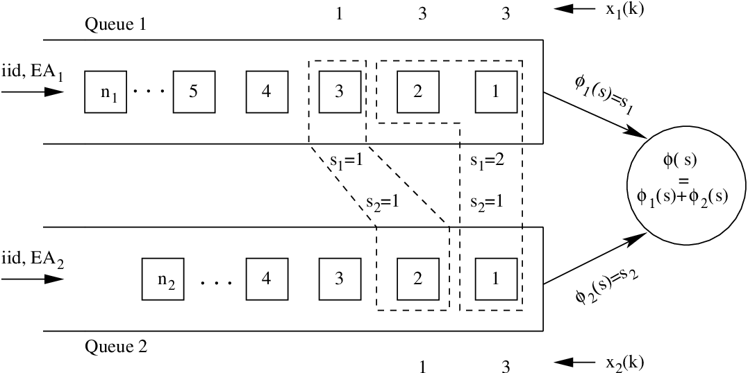
We are interested in characterizing an outerbound to the region of message arrival rate vectors for which the queueing model for joint maximum-likelihood decoding is stable for the class of stationary scheduling policies. In the spirit of the discussion given in Section 1 of Chapter 1, define, for , the rate vector by defining if , and if . With this definition of the rate vector, Theorem 4.1 can be applied to the present context except for the following difference: for and such that , define as the stationary rate at which messages in queue- are assigned to joint messages of the schedule for transmission. Then . That is, .
3 Stability for State-Independent Scheduling Policies
In this section we define the class of stationary state-independent scheduling policies, and then characterize the stability region of message arrival rate vectors for each such policy . To implement a scheduling policy , we further classify class- messages incoming to queue- based on the particular subclass- to be assigned to them.
For and , we say that the pair defines a subclass if . For , the pair does not define a subclass. For each class- message arrival, a subclass- is chosen independently and at random with the fixed probability distribution defined later in (8), and the message is further classified by assigning the subclass- to it. Then messages from source- and are stamped with the subclass- are put into the subclass queue-. For subclass-, let denote the mean number of messages of the subclass- that arrive to the system in a time-slot; obviously . A consequence of class sub-classification is that messages of subclass- will be required to transmit codewords of length , i.e., service requirement gets fixed. The state of the system is defined by the residual service requirements of messages of each subclass present in the system. Thus the definition of the system state in the present context is essentially the same as defined in expression (1) of Chapter 1, except that the state includes a message’s residual service requirement after sub-classification is done. We should observe here that if the pair does not define a subclass.
We now define the notion of a schedule on the set of message subclasses. We define a subclass schedule by a non-negative integer vector such that . We define the set to be the set of all subclass schedules that schedule at most messages in each time-slot. We say that schedule is feasible in state if for all subclasses-. We implement a feasible schedule by serving the first messages at the head of the subclass queue-. We define the ongoing transmission of the schedule in state as the schedule , and is defined as follows: for and ,
We say that a message is fresh if the message has not yet been scheduled for the first time, i.e., the first code letter of the corresponding codeword is yet to be transmitted. The number of fresh messages of subclass- in state is denoted by , and is given by .
We constrain the operation of the system by requiring that there can be at most one ongoing transmission for any schedule in any state . Since first-in-first-out service discipline is used to schedule messages in each subclass queue-, we can determine whether there is an ongoing transmission of the schedule in state by examining the residual service requirement of the messages at the head of the subclass queues-. If there is one ongoing, then for at least one subclass- , we have .
Formally, a policy in this class is defined by (i) an arbitrary probability distribution , and (ii) the mapping . We follow the convention that specification of the policy and of the probability distribution are equivalent. We now define the notion of maximal schedule in the set of the schedule in state .
Definition 3.1 (Sub-Schedule).
For , we write if for each subclass-. We then say that is a sub-schedule of the schedule . The maximal schedule of the schedule in state is defined as follows: for and ,
To implement a state-independent policy , a schedule is chosen independent of the state in each time-slot with probability . Then the subclass schedule
is implemented in state . For the given probability distribution , the mapping induces the probability distribution , which is defined by
Lemma 3.2.
Let , and . For and for each subclass-, define 22 2 denotes the indicator function of the event . if is true, and 0 if is false. , , and . Then the Markov chain is -regular and stable if for each subclass-.
Proof 3.3.
For each subclass-, define to be a partition of such that . Let subclass- messages get generated in state and that the feasible schedule is implemented in the state . Assuming that the chain moves to state , we have
But,
Now consider . Then . Also, .
Assuming for each subclass- , and then applying Lemma 3.2 to and as defined in the statement of Lemma 3.2, we find that the queueing model is -regular. Since there can be at most one ongoing transmission of any schedule in any state , we have . By observing that and , we have
Since for every , existence of finite stationary mean for implies existence of finite stationary mean for . Hence the queueing model is stable.
Let be a splitting probability vector defined by
| (8) |
with the interpretation that is the probability that a class- message request is assigned the schedule .
Lemma 3.4.
For and , the Markov chain is unstable if for at least one subclass-.
Proof 3.5.
For the subclass-, define . Then, we have
and . Consider the partition of the state space defined by . We now consider . Since , we have . Also, . By applying Lemma 3.4 to , , we find that for the Markov chain is unstable.
From Lemma 3.2 and Lemma 3.4, we can easily see that
and that the threshold on is a convex combination of the set of rates . Define . Then is the interior of the convex hull of the rate vectors . We denote the interior of the set by .
Corollary 3.6.
. For any given message arrival rate vector , there exists a state-independent scheduling policy such that the queueing model is stable.
The significance of this Corollary is that, if the queueing model is stable for the message arrival processes and an arbitrary stationary scheduling policy, then there exists a state-independent scheduling policy such that the queueing model is stable for the same message arrival processes .
Proof 3.7.
Suppose that, for some stationary scheduling policy, the queueing model is stable for the message arrival processes . Let be the induced stationary probability distribution on the set of schedules . Let be the stationary probability that no schedule is served in a time-slot. Since the queueing model is stable, the stationary mean residual service for subclass- is finite, and hence .
Let us define a state-independent scheduling policy as follows. For non-empty schedule , define where and . Then, for each subclass-, . That is, for the message arrival processes , the state-independent policy makes the queueing model stable.
4 Information-Theoretic Interpretation to the Stability Region
For a fixed state-independent schedule , i.e., , we know from Lemma 3.2 and Lemma 3.4 that the queueing model is stable if for and , and unstable if for at least one queue such that . We remind the reader that .
In this section, we give the information-theoretic interpretation to the stability region of nat arrival rate vectors for the scenario (S1). A formal statement of this interpretation is made in Theorem 4.1. For , define the code rate vector . In Theorem 4.1, we show the following: (i) for a given joint probability distributions , and message arrival processes such that , we determine a schedule , message alphabet size vector , and a value for the parameter such that the message communication system for , , , and the arrival processes , is stable (i.e., , ); (ii) for any , , and , we show that . Define to be the set of all possible code rate vectors .
Theorem 4.1 (Information-Theoretic Interpretation).
Proof 4.2.
We first show that . Choose an . Then there exists an such that . For and a positive real number , let us first choose and as real numbers such that the product . From Lemma 1.3,
We can see that
where follows from Part (i) of Lemma 7..3, and follows from the fact that and hence . Denote by .
Choose two positive real numbers and such that . Then there exists a such that for all , we have . Now, for a fixed value for such that , there exists a such that for all , we have . Choose an for such that . Define and .
Since and for have to be positive integers, one can, for a given choose for a given , and for a given , and still have the same limit as above.
Chapter 4 Communication Over Degraded Broadcast Channels
The primary intention in this chapter is to demonstrate that the queueing-theoretic model derived for scheduled multiaccess message communication with joint maximum-likelihood decoding in Chapter 3 can be used to model scheduled message communication over degraded broadcast channels with random message arrivals. Due to similarity in the queueing model, we skip queueing model analysis details wherever and whenever possible.
1 The Information-Theoretic Model
A broadcast channel is one through which one source communicates its information to two or more receivers. Formally, a discrete-time stationary memoryless broadcast channel with receivers is defined by a finite input alphabet and finite output alphabets , , and a transition probability law . An assumption inherent in this definition is “no-collaboration” among the receivers. This assumption then allows us to view a broadcast channel as a collection of single-user channels with marginal transition probabilities .
For and integers , let denote the message alphabet of the th source, and define to be a finite set of symbols. For , define the random variables and that take values in the sets and , respectively. Let the th source output be modeled by the random variable that takes values in the set . Some notation specific to this chapter is introduced now. Let and be any two positive integers such that . We define the Cartesian products , and similarly and . Then the vectors , and similarly . Define to be an arbitrary probability assignment on . For , define to be an arbitrary probability assignment on for each . Define to be the product distribution on .
A broadcast channel is said to be degraded if is a Markov chain, i.e., for , there exist probability distributions such that . Fig. 1 shows a degraded broadcast channel through which sources communicate information to the respective receivers. We note that with superposition encoding is a Markov chain, and for , the th channel is a degraded version of the th channel.

Formally, for an integer , the superposition encoder is defined by the mapping , and the decoder at the th receiver is defined by the mapping . The capacity region for general degraded broadcast channels, first conjectured in Cover [3], was established by Bergmans [1]. The converse was established by Bergmans [2] and Gallager [6].
Theorem 1.1 ([1]).
Consider a degraded broadcast channel consisting of component channels (receivers) and represented as the Markov chain
For a given joint probability distribution
define to be the set of rate vectors satisfying for , and . The capacity region is then defined as the convex hull of .
Let denote the codeword chosen for the message vector . Then, for , let denote the th letter of the codeword. The ensemble of broadcast codes we consider here is the same as Bergmans [1] constructed. The random code ensemble is generated in stages as follows. First, consider the ensemble of code words in which each of the letters in each of the code words is independently selected according to the probability assignment . For each of these code words, we choose code words with independent letters from the set according the assignment . That is, conditional on being the th code word, , the probability of a code word , , and , is
Continuing this way, we would have, at the beginning of the th stage, generated codewords. At the end of the th stage, code words will be generated. During the th stage, the process of codeword generation can be modeled by an artificial DMC with transition probability . Each of the -length codewords generated so far are passed through the artificial channel times, thus generating a total of codewords.
A random coding upper bound on message decoding error probabilities for the two receiver degraded broadcast channel was derived in [6]. Here we extend that result to a degraded broadcast channel with arbitrary number of receivers. The objective of the decoder at the th receiver is to compute an estimate 11 1 Since, for , th source message is estimated at the th receiver, we denote an estimate of the th source at the th receiver by . of . This is achieved by successive decoding, with the th decoder first decoding and then subtracting the signals intended for the users with noisier channels before decoding its own. Let the event be the event that the decoder at the th receiver makes an error in decoding the th source. The probability of error for the th decoder then is .
For and , let denote the probability of decoding the th source at the th receiver incorrectly conditioned on th sources being decoded correctly, and the expectation of over the ensemble of broadcast codes. The transition probability of the effective channel between , , and , , for and , is given by
One can then consider as being produced by passing through a DMC with transition probability law . In the following Theorem 1.2, we compute an upper bound on the expected probability of the event .
Theorem 1.2.
For , (i) and, (ii) for , the expected probability given that the joint message is encoded is upper bounded as
| (1) | |||||
| for , and | |||||
Proof 1.3.
To prove Part (i), consider the joint ensemble formed by the random vectors and . Define the event as the set of all sample points in this joint ensemble such that . We now show that can be expressed as a union of mutually exclusive and collectively exhaustive events. For , define the events as follows: , and for , , and finally . Then . But, for , we have that , and for , . Hence, for , we have
and for , . Hence .
Next we prove Part (ii). Proof of Part (ii) is a straightforward extension of the proof given in [6]. To derive an upper bound on , we first condition the event of this type of error upon the code word chosen for the message vector . Let be the probability of this error event. That is, is the probability that
for some such that and in the conditional ensemble, and is independently chosen with the probability assignment . The coding Theorem 5.6.1 [5] applies to this situation, yielding
Next, is the expected value of over and . Since the bound is independent of , we average only over .
For , is the expected probability of error in decoding source- when it is communicated over a discrete memoryless channel with transition probability law and channel input distribution . Thus, the probability of decoding error is bounded above by the usual results for decoding on a DMC (Theorem 5.6.1 [5]).
2 The Queuing-Theoretic Model
The queuing-theoretic model for a receiver degraded broadcast
channel that we derive is similar to the queuing-theoretic model we
derived for the source multiaccess channel with joint
maximum-likelihood decoding for the scenario (S1) in
Chapter Scheduling for Stable and Reliable Communication
over Multiaccess Channels
and Degraded Broadcast Channels.
The similarity can be seen as follows: we maintained a queue for each
source in the case of the multiaccess channel, whereas we maintain a
queue for each receiver at the transmitter in the case of the degraded
broadcast channel. Hence, messages that arrive at the transmitter and
are intended for receiver- are put into queue . For , let (as defined in
Chapter 1) be the set of schedules that encode at most
messages for transmission.
Under the scenario (S3), a schedule defines product message alphabets such that for each of the receivers. Hence we need to redefine the coding rate (Eq. (1) in Theorem 1.2) for receiver- as , thus emphasizing the dependence of effective message alphabet size on schedule . Let denote the random coding upper bound for the th receiver under the schedule , and the set of tolerable message decoding error probabilities. For and such that , define to be the smallest positive integer such that . In the following Lemma 2.1, we derive an upper bound and a lower bound on .
Lemma 2.1.
Proof 2.2.
The arguments leading to the above bounding are similar to the arguments given in the proof of Lemma 1.3. Hence we skip the detailed proof.
Lemma 2.3.
Let . Then for .
Proof 2.4.
Since , we first note that . Since, is independent of and , we conclude that . Now, we observe that
Thus, . Since is the smallest positive integer
such that
, we have that .
Define . Then is the smallest positive integer such that for .
At this point we should observe that, at the beginning of each time-slot, we need to inform the receivers about the schedule that will be implemented in that time-slot. This is achieved by assuming that synchronized common randomness is available at the transmitter and receivers to generate schedules with the distribution (and also the code books). Then, only those receivers- such that will decode their respective received signals. But, in a particular time-slot, it may happen that a schedule is chosen for transmission and enough messages of each class required by the schedule are not present in the system. To resolve this problem, we can substitute each such “missing message” by a message with null value, thus embedding control information in information from sources. Inclusion of the null message in increases the cardinality by one and may have the effect of increasing accordingly, thus reducing the throughputs achievable for finite message lengths. But this effect disappears in the asymptotic limit .
However, in the following we assume that this control information is passed to the receivers over an error-free control channel, so that the queueing model analysis presented in Chapter 3 applies in the present context without modifications.
Define the service requirement of a message under schedule , and the service quantum available to queue at a discrete-time instant, as in Chapter 3. Then (i) the notion of rate vectors and the outer bound derived in Section 2 on the stability region of message arrival rate vectors achievable by stationary scheduling policies, and (ii) the definition of state-independent scheduling policies and their stability analysis described in Section 3 and the following Corollary 3.6 therein, apply verbatim to the queueing model for the degraded broadcast channel.
3 Information-Theoretic Interpretation to the Stability Region
For a fixed state-independent schedule , i.e., , we know from Theorem 3.2 and Theorem 3.4 that the queueing model is stable if for , and unstable if for at least one queue .
In this section, we give the information-theoretic interpretation to the stability region of nat arrival rate vectors for the scenario (S3). A formal statement of this interpretation is made in Theorem 3.1. For , define the code rate vector . In Theorem 3.1, we show the following: (i) for a given joint probability distributions , and message arrival processes such that , we determine a schedule , message alphabet size vector , and a value for the parameter such that the message communication system for , , , and the arrival processes , is stable (i.e., , ); (ii) for any , , and , we show that . Define to be the set of all possible code rate vectors .
Theorem 3.1 (Information-Theoretic Interpretation).
Proof 3.2.
We first show that . Choose an . Then there exists an such that . For and a positive real number , let us first choose and as real numbers such that the product . From Lemma 2.1,
We can see that
where follows from Part (i) of Lemma 7..4, follows from the fact that and hence , and follows from the data processing inequality (Theorem 2.8.1 in [4]) applied to the Markov chain . Denote by .
Choose two positive real numbers and such that . Then there exists a such that for all , we have . Now, for a fixed value for such that , there exists a such that for all , we have . Choose an for such that . Define and .
Since and for have to be positive integers, one can, for a given choose for a given , and for a given , and still have the same limit as above.
Chapter 5 Conclusion
We have developed a unified framework, namely, multiclass discrete-time processor-sharing queueing model of Chapter 1, to analyze stability of scheduled message communication over multiaccess channels with either independent decoding or joint decoding, and over degraded broadcast channels. Under this framework, we modeled both the random message arrivals and the subsequent reliable communication by suitably combining techniques from queueing theory and information theory.
For scheduled message communication over a multiaccess channel with independent maximum-likelihood decoding, we showed the following.
- 1.
For finite message lengths, inner bounds and outer bounds to the message arrival rate stability region are derived. For arrival rates within the inner bounds, we show finiteness of the stationary mean for the number of messages in the system and hence for message delay. For the case of equal received signal powers, with sufficiently large SNR, the stability threshold increases with decreasing maximum number of simultaneous transmissions (see Fig. 2).
- 2.
When message lengths are large, the information arrival rate stability region has an interpretation in terms of interference-limited information-theoretic capacities. For the case of equal received powers, this stability threshold is the interference-limited information-theoretic capacity.
- 3.
We propose a class of stationary policies called state-independent scheduling policies, and then show that they achieve this asymptotic information arrival rate stability region.
- 4.
In the asymptotic limit corresponding to immediate access, the stability region for Gaussian encoding and non-idling scheduling policies is shown to be identical irrespective of received signal powers. This observation essentially shows that transmit power control is not needed. We show that, in the asymptotic limit corresponding to immediate access and large message lengths, a spectral efficiency of 1 nat/s/Hz is achievable with non-idling scheduling policies (see Fig 3).
For scheduled message communication over multiaccess channels with joint maximum-likelihood decoding, we derived an outer bound to the stability region of message arrival rate vectors achievable by the class of stationary scheduling policies. Then we showed for any message arrival rate vector that satisfies the outer bound, that there exists a stationary “state-independent” policy that results in a stable system for the corresponding message arrival processes. Finally, we showed that for any achievable rate vector in the capacity region of a multiaccess channel, there exists a scheduling strategy and message lengths for that rate vector such that the message system with random message arrivals is stable.
We showed that the queueing model derived in the case of multiaccess channels with joint maximum-likelihood decoding can be used to model scheduled message communication over degraded broadcast channels with superposition encoding and successive decoding. We then showed that the results obtained from stability analysis of multiaccess channels apply verbatim to the degraded broadcast channels. We also showed that for any achievable rate vector in the capacity region of a degraded broadcast channel , there exists a scheduling strategy and message lengths for that rate vector such that the broadcast message system with random message arrivals is stable.
Chapter 6 Drift theorems for Positive Recurrence and Transience
Drift theorems for classification (in terms of transience, positive recurrence and null recurrence) of discrete-time Markov chains taking values in a general state space have been stated in [11]. We rewrite the theorems here for discrete-time Markov chains taking values in a countable state space.
[11] defines a measure, , on the state space, , which is called the ‘maximal irreducibility measure’. For an irreducible Markov chain taking values in a countable state space, the measure is generated by a counting measure on [p. 88, [11]]. Hence, an irreducible Markov chain taking values in a countable state space, , is -irreducible with , where denotes a state in the countable state space.
[11] defines the set, , [p. 55, [11]] as some -algebra on the general state space, . For a countable state space, without loss of generality, we take this -algebra as the set of all subsets of . Then, defined as , in the case of irreducible Markov chains on a countable state space, becomes the set of all non-empty subsets of , i.e., .
We now rewrite the theorems stated in [11] for discrete-time Markov chains taking values in a countable state space.
Appendix 6.A Theorem for Positive Recurrence
Theorem 11.3.4 stated in [11] can be written as follows. Suppose
and is petite, and an everywhere finite function
satisfies
11
1
is the expected drift of the function, , in state
., then
is positive Harris recurrent.
Finite sets in a countable state space are petite [p.192, [11]]. A chain is Harris recurrent if every set in is Harris recurrent [p.200, [11]]. If a set is Harris recurrent then it is recurrent [p.201, [11]]. Positivity for a -irreducible Markov chain means existence of an invariant probability measure for the chain [p.230, [11]]. Thus, for an irreducible Markov chain on a countable state space positive Harris recurrence implies positive recurrence. The theorem stated above, together with the interpretations made before, can then be written in the context of Markov chains in a countable state space as follows.
An irreducible Markov chain, , is positive recurrent
if there exists a finite subset of and an everywhere finite function
bounded on such that
a. , and
b. .
Appendix 6.B Theorem for Transience
Theorem 8.0.2 (i) stated in [11] is as follows : Suppose is a -irreducible chain. The chain, , is transient iff there exists a bounded non-negative function, , and a set such that for all , , and .
Thus, the theorem stated above, together with the interpretations made before, can be written in the context of Markov chains in a countable state space as follows :
An irreducible Markov chain, , is transient iff there exists a bounded non-negative function, , and a non-empty set such that for all , , and such that .
Chapter 7 Two properties of and
In this appendix, we state two properties of and used in the random coding upper bounds on expected decoding error probabilities for joint maximum-likelihood decoding for the multiaccess channel (Chapter 3) and the degraded broadcast channel (Chapter 4), respectively. These properties are derived by a straightforward application of Theorem 5.6.3. in [5] for the respective communication channels.
For a finite set , define a random variable that takes values in the set with the probability distribution . Let and be the input and output of a DMC, and for consider the input distributions and the transition probability law . Then is the probability distribution induced on the output alphabet . Define , and then .
Lemma 7..1.
, and is a decreasing function for .
Proof 7..2.
Define . It is easy to observe that . We have
Since , and , we therefore have .
Define for . Then . Now, define for . Then we can see that , and for (Theorem 5.6.3 in [5]). So we conclude that is a decreasing function in , and since we have that for . Equivalently, for . This establishes that is a decreasing function in and that for .
We now state the following two Lemmas. Lemma 7..3 results when Lemma 7..1 is applied to in Theorem 1.2. Part (i) and (ii) of Lemma 7..4 result if we apply Lemma 7..1 to in Theorem 1.2.
Lemma 7..3.
Consider a source multiple-access channel with joint maximum-likelihood decoding. Then (i) for , and (ii) for .
Lemma 7..4.
Consider a -receiver degraded broadcast channel represented as the Markov chain . Then (i) , (ii) for .
References
- [1] P. P. Bergmans. “Random Coding Theorem for Broadcast Channels with Degraded Components”. IEEE Transactions on Information Theory, 19(2):197–207, March 1973.
- [2] P. P. Bergmans. “A Simple Converse for Broadcast Channels with Additive White Gaussian Noise”. IEEE Transactions on Information Theory, IT-20:279–280, March 1974.
- [3] T. M. Cover. “Broadcast Channels”. IEEE Transactions on Information Theory, IT-18(1):2–14, January 1972.
- [4] T. M. Cover and J. A. Thomas. Elements of Information Theory. Wiley Series in Telecommunications. John Wiley & Sons, Inc., 1991.
- [5] R. G. Gallager. Information Theory and Reliable Communication. John Wiley and Sons, Inc, 1968.
- [6] R. G. Gallager. “Capacity and Coding for Degraded Broadcast Channels”. Problemy Peredachi Informatsii, 10(3):3–14, July-September 1974.
- [7] R. G. Gallager. “A Perspective on Multiaccess Channels”. IEEE Transactions on Information Theory, IT-31(2):124–142, March 1985.
- [8] Tommy Guess and Mahesh K. Varanasi. “Error Exponents for Maximum-Likelihood and Successive Decoders for the Gaussian CDMA Channel”. IEEE Transactions on Information Theory, 46(4):1683–1691, July 2000.
- [9] S. V. Hanly and D. Tse. “Multi-Access Fading Channels:Part II: Delay-Limited Capacities”. IEEE Transactions on Information Theory, 44(7):2816–2831, Nov. 1998.
- [10] S.P. Meyn. “Stability, Performance Evaluation, and Optimization”, chapter in Handbook of Markov Decision Processes (E.A. Feinberg and A. Shwartz, ed.). Kluwer Academic, 2002.
- [11] S.P. Meyn and R.L. Tweedie. Markov Chains and Stochastic Stability. Springer Verlag, 1993.
- [12] U. Mukherji, S. V. Ramdurg, KCV Sayee, V. Dua, and T. N. Krishnan. ”Multi-access Poisson Traffic Communication with Random Coding, Independent Decoding and Unequal Powers”. Proceedings of IEEE Information Theory Workshop, page 220, October 2002.
- [13] I.E Telatar. “Multi-access Communications with Decision Feedback Decoding”. Ph.D. Dissertation, Report CICS-TH-33, Dept. of Electrical Engineering and Computer Science, Massachusetts Institute of Technology, 1992.
- [14] I.E. Telatar. “Combining Queueing Theory with Information Theory for Multi-access with Joint Decoding”. In Proceedings of IEEE Information Theory Workshop, page 51, St. Louis, April 1995.
- [15] I.E. Telatar and R.G. Gallager. “Combining Queueing Theory with Information Theory for Multiaccess”. IEEE Journal on Selected Areas in Communications, 13(6):963–969, August 1995.