On-line topological simplification
of weighted graphs

Floris Geerts Peter Revesz Thanks: Work done while on a sabbatical leave from the University of Nebraska-Lincoln. Work supported in part by USA NSF grants IRI-9625055 and IRI-9632871. Jan Van den Bussche

¹ Hasselt University/Transnational University Limburg
² University of Nebraska-Lincoln
³ University of Edinburgh

Abstract

We describe two efficient on-line algorithms to simplify weighted graphs by eliminating degree-two vertices. Our algorithms are on-line in that they react to updates on the data, keeping the simplification up-to-date. The supported updates are insertions of vertices and edges; hence, our algorithms are partially dynamic. We provide both analytical and empirical evaluations of the efficiency of our approaches. Specifically, we prove an $O(\log n)$ upper bound on the amortized time complexity of our maintenance algorithms, with $n$ the number of insertions.

1 Introduction

Many GIS applications involve data in the form of a network, such as road, railway, or river networks. It is common to represent network data in the form of so-called polylines. A polyline consists of a sequence of consecutive straight-line segments of variable length. Polylines allow for the modeling of both straight lines and curved lines. A point on a polyline in which exactly two straight-line segments meet, is called a regular point. Regular points are important for the modeling of curved lines. Indeed, to represent accurately a curved line by a polyline, one needs to use many regular points. Curved lines often occur in river networks, or in road networks over hilly terrain.

We illustrate this in Figure 1 in which we show a part of the road network in the Ardennes (Belgium). In this hilly region, many bended roads occur. As can be seen in the Figure, there is an abundance of regular points — which is often the case in real network maps [14].

Refer to caption — Figure 1: Road network in two villages Tenneville (top) and La Roche (bottom) in the Belgian Ardennes. Black points are non-regular points; gray points are regular. We see that the number of gray points is very high.

Although regular points are necessary to model the reality accurately, for many applications they can be disregarded. More specifically, for topological queries such as path queries, one can “topologically simplify” the network by eliminating all regular points; and answer the query (more efficiently) on the much simplified network. Even when the network contains distance information, one still can topologically simplify the network, but maintain the distance information, as we will show in the present paper. More generally, we work with arbitrary weight information.

Thus, the simplification of a network contains in a compact manner the same topological and distance information as the original network. Such “lossless topological representations” have been studied by a number of researchers [7, 10, 11]. For example, initial experiments reported by Segoufin and Vianu have shown drastic compression of the size of the data by topological simplification. (The inclusion of distance information is new to the present paper.)

Of course, if we want to answer queries using the simplified network instead of the original one, we are faced with the problem of on-line maintenance of the simplified network under updates to the original one. This problem is important due to the dynamic character of certain network data. For example, suppose that there is a huge snowstorm which makes all roads unusable. As a result, many snow clearing crews are sent to all parts of the city. They continuously report back to a central station the road segments that they have cleared. The central station also continuously updates its map of the usable network of roads. Moreover, big arteries are cleared first, and therefore, the usable network will have a high percentage of regular vertices in the initial stages. While the snow is being cleared, thousands of people may query the database of the central station to find out what is the shortest path they can take using the already cleared roads. Analogous applications requiring on-line monitoring involve traffic jams in road networks, or downlinks in computer networks.

Two of us have reported on an initial investigation of this problem [5]. The result was a maintenance algorithm that was fully-dynamic, i.e., insertions and deletions of edges and vertices are allowed. This algorithm, however, is (in certain “worst cases”) not any better than redoing the simplification from scratch after every update, resulting in an $O(n^{2})$ time algorithm, where $n$ is the number of updates. This is clearly not very practical.

The present paper proposes two very different algorithms for on-line topological simplification:

1.

Renumbering Algorithm, which relies on the numbering and renumbering of the regular vertices, takes on the average, only logarithmic time per edge insertion to keep the simplified network up-to-date; and
2.

Topology Tree Algorithm, is based on the topology tree data structure of Frederickson [3] and has the same time complexity $O(n\log(n))$ .

Neither algorithm makes any assumptions on the graph, such as planarity and the like. Real-life network data is often not planar (e.g., in a road or railway network, bridges occur). The presented algorithms are only semi-dynamic, in that they can react efficiently to insertions (of vertices and edges), but not to deletions. Insertions are sufficient for many applications (such as the snow clearing mentioned above, were simply more and more road segments become available again), but for applications requiring also deletion, the Topology Tree Algorithm easily can be extended to also react correctly to edge deletions.

We have performed an empirical comparison of the Renumbering Algorithm and the Topology Tree Algorithm using random, non-random and two real data sets.

This paper is further organized as follows. Basic definitions are given in Section 2. The general description of the on-line simplification algorithm is described in Section 3. In Section 4, we describe the Renumbering Algorithm, and in Section 5, the Topology Tree Algorithm is described. The empirical comparison of both algorithms is presented in Section 6.

2 Basic Definitions

Consider an undirected graph without self-loops $G=(V,E,\lambda)$ with weighted edges; the weights of the edges are given by a mapping $\lambda:E\rightarrow{\bf R}^{+}$ . We will use the following definitions:

1.

A vertex $v$ is regular if and only if it is adjacent to precisely two edges.
2.

A vertex that is not regular is called singular.
3.

A path between two singular vertices that passes only through regular vertices is called a regular path.

We assume that the graph $G$ does not contain regular cycles: cycles consisting of regular vertices only.

The simplification $G_{s}=(V_{s},E_{s},\lambda_{s})$ of $G$ is a multigraph with self-loops and weighted edges, which is obtained as follows: (see Figure 1)

1.

$V_{s}$ , the set of nodes of $G_{s}$ , consists of all singular vertices of $G$ .
2.

$E_{s}$ , the set of edges of $G_{s}$ , formally consists of all regular paths of $G$ . Every regular path between two singular vertices $v$ and $w$ represents a topological edge in $G_{s}$ between $v$ and $w$ . There might be multiple regular paths between two singular vertices, so in general $G_{s}$ is a multigraph.
3.

the weight $\lambda_{s}(e)$ of a topological edge $e$ is equal to the sum of all weights of edges on the regular path corresponding to $e$ .

In the following, when a particular regular path $e$ between two singular vertices $v$ and $w$ is clear from the context, we will abuse notation and conveniently denote the topological edge $e$ by $\{v,w\}$ .

3 Online Simplification: General Description

We consider only insertions of a new isolated vertex and insertions of edges between existing vertices in the graph $G$ (other more complex insertion operations can be translated into a sequence of these basic insertion operations). The insertion of an isolated vertex is handled trivially, i.e., we insert it into $V_{s}$ .

For the insertion of an edge we distinguish between six cases that are explained below. The left side of each figure shows the situation before the insertion of the edge $\{x,y\}$ , drawn as the dotted line, and the right side shows the situation after the insertion. The topological edges are drawn in thick lines.

Case 1: Vertices $x$ and $y$ are both singular and $\deg(x)\neq 1$ and $\deg(y)\neq 1$ .

Then the edge $\{x,y\}$ is also inserted in $G_{s}$ .
Case 2: Vertices $x$ and $y$ are both singular and one of them, say $x$ , has degree one.

Let $\{z,x\}$ be the edge in $G_{s}$ adjacent to $x$ . Extend this edge the new edge $\{z,y\}$ in $G_{s}$ , putting $\lambda_{s}(\{z,y\}):=\lambda_{s}(\{z,x\})+\lambda(\{x,y\})$ . Note that $x$ becomes a regular vertex after the insertion.
Case 3: Vertices $x$ and $y$ are both singular and $\deg(x)=\deg(y)=1$ .

Let $\{z_{1},x\}$ ( $\{z_{2},y\}$ ) be the edge in $G_{s}$ adjacent with $x$ ( $y$ ). (Since we disallow regular cycles in $G$ , we have $z_{1}\neq y$ and $z_{2}\neq x$ .) Then merge the edges $\{z_{1},x\}$ and $\{y,z_{2}\}$ in $G_{s}$ into a single, new edge $\{z_{1},z_{2}\}$ in $G_{s}$ , putting $\lambda_{s}(\{z_{1},z_{2}\}):=\lambda_{s}(\{z_{1},x\})+\lambda_{s}(\{y,z_{2}\})+\lambda(\{x,y\})$ .
Case 4: One of the vertices $x$ and $y$ is regular, say $x$ , and the other vertex, $y$ , is singular and has degree one.

First, the edge $\{z_{1},z_{2}\}$ of $G_{s}$ which corresponds to the regular path between $z_{1}$ and $z_{2}$ on which $x$ lies, must be split into two new edges $\{z_{1},x\}$ and $\{x,z_{2}\}$ of $G_{s}$ . Here, we put $\lambda_{s}(\{z_{1},x\}):=\sum\lambda(\{u,v\})$ , where the summation is over all edges in $G$ on the regular path from $z_{1}$ to $x$ . We similarly define $\lambda_{s}(\{x,z_{2}\})$ . Secondly, let $\{z_{3},y\}$ be the edge in $G_{s}$ adjacent to $y$ . Then we extend this edge to a new edge $\{z_{3},x\}$ in $G_{s}$ , putting, $\lambda_{s}(\{x,z_{3}\}):=\lambda_{s}(\{y,z_{3}\})+\lambda(\{x,y\})$ .

A special subcase occurs when $z_{1}=z_{2}$ . In that case, the two paths from $x$ to $z_{1}$ give rise to two different edges from $x$ to $z_{1}$ in $G_{s}$ (recall that $G_{s}$ was defined as a multigraph).
Case 5: One of the vertices, say $x$ , is regular and the other one, $y$ , is singular with degree not equal to one.

Then we split exactly as in case 4, and now we also insert $\{x,y\}$ as a new edge in $G_{s}$ .
Case 6: Both $x$ and $y$ are regular.

Now, two splits must be performed.

As can be seen in the above description, if no regular vertices are involved, then the update on the graph $G$ translates in a straightforward way to an update on the simplification $G_{s}$ . It is only in cases 4, 5, and 6, that the update on the graph $G$ involves vertices which have no counterpart in the simplification $G_{s}$ . In these cases, we need to find the edge to split and the weights of the topological edges created by the split. Consequently, the problem of maintaining the simplification $G_{s}$ of a graph $G$ amounts to two tasks:

•

Maintain a function find topological edge, which takes a regular vertex as input, and outputs the topological edge whose corresponding regular path in $G$ contains the input vertex.
•

Maintain a function find weights which outputs the weights of the edges created when a topological edge is split at the input vertex.

In an earlier, naive approach [5], we only discussed the function find topological edge. It worked by storing for each regular vertex a direct pointer to its topological edge. This made the topological edge accessible in constant time, but the maintenance of the pointers under updates can be very inefficient in the worst case. We next describe two algorithms which are more efficient. Both algorithms keep the simplification of a graph up-to-date when the graph is subject to edge insertions only.

4 Online Simplification: Renumbering Algorithm

In this section we introduce an algorithm for keeping the simplification of a graph up-to-date when this graph is subject to edge insertions. We first show how the topological edges can be found efficiently.

4.1 Assigning numbers to the regular vertices

We number the regular vertices, that lie on a regular path, consecutively. The numbers of the regular vertices on any regular path will always form an interval of the natural numbers. The Renumbering Algorithm will maintain two properties:

Interval property:: the assignment of consecutive numbers to consecutive regular points;
Disjointness property:: different regular paths have disjoint intervals.

We then have a unique interval associated with each regular path, and hence with each topological edge of size $>0$ . Moreover, we choose the minimum of such an interval as a unique number associated with a topological edge. Specifically, the minimal number serves as a key in a dictionary. Recall that in general, a dictionary consists of pairs $\langle\mbox{key},\mbox{item}\rangle$ , where the item is unique for each key. Given a number $k$ , the function which returns the item with the maximal key smaller than $k$ can be implemented in $O(\log N)$ time, where $N$ is the number of items in the dictionary [1].

The items we use contain the following information.

1.

An identifier of the topological edge associated with the key.
2.

The number of regular vertices on the regular path corresponding to this topological edge.
3.

An identifier of the regular vertex that has the key as number on this path.

In Figure 2 we give an example of a dictionary containing three keys, corresponding to the three topological edges in the simplification $G_{s}$ of the graph $G$ .

4.2 Maintaining the numbers of the regular vertices

We must now show how to maintain this numbering under updates, such that the interval and disjointness properties mentioned above remain satisfied.

Actually, only in case 3 in Section 3 we need to do some maintenance work on the numbering. Indeed, by merging two topological edges, the numbering of the regular vertices is no longer necessarily consecutive. We resolve this by renumbering the vertices on the shorter of the two regular paths. Note that the size of a regular path is stored in the dictionary item for that path.

In order to keep the intervals disjoint, we must assume that the maximal number of edge insertions to which we need to respond is known in advance. Concretely, let us assume that we have to react to at most $\ell$ update operations. This assumption is rather harmless. Indeed, one can set this maximum limit to a large number. If it is eventually reached, we restart from scratch. A regular path is “born” with at most two regular vertices on it. Every time a new regular path is created, say the $k$ th time, we assign the number $2k\ell$ to one of the two regular vertices on it. Hence, newly created topological edges correspond to numbers which are $2\ell$ apart from each other. Since a newly created topological edge can become at most $\ell-1$ vertices longer, no interference is possible.

4.3 Finding the topological edge

Consider that we are in one of the cases 4–6 described in Section 3, where we have to split the topological edge at vertex $x$ . We look at the number of $x$ , say $k$ , and find in the dictionary the item associated with the maximal key smaller than $k$ . This key corresponds to the interval to which $k$ belongs, or equivalently, to the regular path to which $x$ belongs. In this way we find the topological edge which has to be split, since this edge is identified in the returned item.

The numbering thus enables us to find an edge in $O(\log m^{\prime})$ time, where $m^{\prime}$ is the number of edges in $G_{s}$ which correspond to a regular path passing through at least one regular vertex. Because $m^{\prime}$ is at most $m$ , the number of edges in $G$ , we obtain:

Proposition 4.1.

Given a regular vertex and its number, the dictionary returns in $O(\log m)$ time the topological edge corresponding to the regular path on which this regular vertex lies.

We next show how, when a topological edge is split, we can quickly find the weights of the two new edges created by the split.

4.4 Assigning weights to the regular vertices

The weight of a regular vertex $v$ will be denoted by $\lambda^{\ast}(v)$ . Weights will be assigned to the regular vertices such that if $v$ and $w$ are two consecutive regular vertices with weights $\lambda^{\ast}(v)$ and $\lambda^{\ast}(w)$ respectively, then $\lambda(\{v,w\})=|\lambda^{\ast}(v)-\lambda^{\ast}(w)|$ .

4.5 Maintaining the weights of regular vertices

The maintenance of the weights of regular vertices under edge insertions is easy. It requires only constant time when a topological edge is extended. Indeed, let $\{x,y\}$ be a topological edge, and suppose that we extend this edge by inserting $\{y,z\}$ . Let $u$ be the regular vertex adjacent to $y$ . Then,

•

if $\lambda^{\ast}(u)<0$ , then $\lambda^{\ast}(y):=\lambda^{\ast}(u)-\lambda(\{u,y\})$ .
•

if $\lambda^{\ast}(u)\geqslant 0$ , and no regular vertex with a positive weight is adjacent to $u$ , then $\lambda^{\ast}(y):=\lambda^{\ast}(u)+\lambda(\{u,y\})$ . Otherwise, let $v$ be the regular vertex adjacent to $u$ . If $\lambda^{\ast}(v)>\lambda^{\ast}(u)$ , then let $\lambda^{\ast}(y)=\lambda^{\ast}(u)-\lambda(\{u,y\})$ , else let $\lambda^{\ast}(y)=\lambda^{\ast}(u)+\lambda(\{u,y\})$ .

When a topological edge is split, no adjustments to the weight of the remaining regular vertices is needed at all. However, when two topological edges are merged we need to adjust the weights of the regular vertices on the shortest of the two regular paths, as shown in Figure 3. This adjustment of the weights can clearly be done simultaneously with the renumbering of the vertices.

4.6 Finding the weights

The weights of regular vertices now enable us to find the weights of the two edges created by a split of a topological edge in logarithmic time. Indeed, given the number of the regular vertex where the split occurs, we search in the dictionary which topological edge needs to be split; call it $\{z_{1},z_{2}\}$ . In the returned item we find the vertex which has the minimal number of the vertices on the regular path corresponding to $\{z_{1},z_{2}\}$ . Denote this vertex with $u$ which is adjacent to either $z_{1}$ or $z_{2}$ . We assume that $u$ is adjacent to $z_{1}$ , the other case being analogous. The weight of the two new topological edges $\{z_{1},x\}$ and $\{x,z_{2}\}$ can be computed easily:

•

$\lambda(\{z_{1},x\}):=\lambda(\{z_{1},u\})+|\lambda^{\ast}(u)-\lambda^{\ast}(x)|$ ; and
•

$\lambda(\{x,z_{2}\}):=\lambda(\{z_{1},z_{2}\})-\lambda(\{z_{1},x\})$ .

If only one regular vertex remains on a regular path after a split, or a regular vertex becomes singular, then the weight of this vertex is set to $0$ . This can all can be done in constant time, after the topological edge which needs to be split has been looked up in the dictionary.

4.7 Complexity analysis

By the amortized complexity of an on-line algorithm [13, 8], we mean the total computational complexity of supporting $\ell$ updates (starting from the empty graph), as a function of $\ell$ , divided by $\ell$ to get the average time spent on supporting one single update. We will prove here that the Renumbering Algorithm has $O(\log\ell)$ amortized time complexity. We only count edge insertions because the insertion of an isolated vertex has zero cost.

Theorem 4.1.

The total time spent on $\ell$ updates by the Renumbering Algorithm is $O(\ell\log\ell)$ .

Proof.

If we look at the general description of the Renumbering Algorithm, we see that in each case only a constant number of steps are performed. These are either elementary operations on the graph, or dictionary lookups. There is however one important exception to this. In cases where we need to merge two topological edges, the renumbering of regular vertices (and simultaneous adjustment of their weights) is needed. Since every elementary operation on the graph takes constant time, and every dictionary lookup takes $O(\log\ell)$ time, all we have to prove is that the total number of vertex renumberings is $O(\ell\log\ell)$ .

A key concept in our proof is the notion of a super edge (see Figure 4). Super edges are sets of topological edges which can be defined inductively: initially each topological edge (with one or two regular vertices on it) is a member of a separate super edge. If a member ${\bf a}$ of a super edge ${\bf A}$ is merged with a member ${\bf b}$ of another super edge ${\bf B}$ , then the two super edges are unioned together in a new super edge ${\bf C}$ and ${\bf a}$ and ${\bf b}$ are merged into a new member ${\bf c}$ of the new super edge ${\bf C}$ . If a member ${\bf d}$ of a super edge is split into ${\bf e}$ and ${\bf f}$ , then both ${\bf e}$ and ${\bf f}$ will belong to the same super edge as ${\bf d}$ did. The important property of super edges is that the total number of vertices can only grow. We call this number the size of a super edge. A split operation does not affect the size of super edges, while merge operations can only increase it.

It now suffices to show that the total number of vertex renumberings in a super edge of size $\ell$ is $\ell\log\ell$ . We will do this by induction.

The statement is trivial for $\ell=0$ , so we take $\ell>0$ . We may assume that the $\ell$ th update involves a merge of two topological edges, since this is the only update for which we have to do renumbering. Suppose that the sizes of the two super edges being unioned are $\ell_{1}$ and $\ell_{2}$ . Without loss of generality assume that $\ell_{1}\leq\ell_{2}$ . Hence, according to the Renumbering Algorithm which renumbers the shortest of the two, we have to do $2\ell_{1}$ renumbering steps: $\ell_{1}$ to assign new numbers, and $\ell_{1}$ to assign new weights. The size of the new super edge will be $\ell=\ell_{1}+\ell_{2}$ . By the induction hypothesis, the total number of renumberings already done while building the two given super edges are $\ell_{1}\log\ell_{1}$ and $\ell_{2}\log\ell_{2}$ . It is known ([12]) that

2\min\{x,1-x\}\leqslant\ x\log\frac{1}{x}+(1-x)\log\frac{1}{1-x},

(1)

for $x\in[0,1]$ . Define $x=\ell_{1}/\ell$ . By (1), we then obtain the inequality

\displaystyle\ell_{1}\log\ell_{1}+\ell_{2}\log\ell_{2}+2\ell_{1}

\displaystyle\leqslant

\displaystyle\ell\log\ell,

as had to be shown. ∎

To conclude this section, we recall from Section 4.2 that the maximal number assigned to a regular vertex is $2\ell^{2}$ . So, all numbers involved in the Renumbering Algorithm take only $O(\log\ell)$ bits in memory. Theorem 4.1 assumes the standard RAM computation model with unit costs. If logarithmic costs are desired, the total time is $O(\ell\log^{2}\ell)$ .

5 Online-Simplification: Topology Tree Algorithm

In this section we introduce another algorithm for keeping the simplification of a graph up-to-date when this graph is subject to edge insertions. We only describe the case of edge insertion, but it is straightforward to extend the Topology Tree Algorithm to a fully dynamic algorithm, which can also react to deletions. The algorithm uses a direct adaptation of the topology-tree data structure introduced by Frederickson [3, 4]. This data structure has been used extensively in other partially and fully dynamic algorithms [6].

We first show how the topological edge can be found efficiently.

5.1 Regular multilevel partition

We define a cluster as a set of vertices. The size of a cluster is the number of vertices it contains. A regular cluster is a cluster of size at most two, containing adjacent regular vertices. A regular partition of a graph $G$ is a partition of the set $V_{r}$ of regular vertices, such that for any two adjacent regular vertices $v$ and $w$ , the following holds:

•

either $v$ and $w$ are in the same regular cluster $\mathcal{C}$ ; or
•

$v$ and $w$ are in different regular clusters $\mathcal{C}_{v}$ and $\mathcal{C}_{w}$ , and at least one of these regular clusters has size two.

A regular multilevel partition of a graph $G$ is a set of partitions of $V_{r}$ that satisfy the following (see Figure 5):

1.

For each level $i=0,1,\ldots,k$ , the clusters at level $i$ form a partition of $V_{r}$ .
2.

The clusters at level $0$ form a regular partition of $V_{r}$ .
3.

The clusters at level $i$ form a regular partition when viewing each cluster at level $i-1$ as a regular vertex.

A regular forest of a graph $G$ is a forest based on a regular multilevel partition of $G$ . We focus on the construction of a single tree in the forest corresponding to a single regular path. A single tree is constructed as follows (see Figure 6).

1.

A vertex at level $i$ in the tree represents a cluster at level $i$ in the regular multilevel partition.
2.

A vertex at level $i>0$ has children that represent the clusters at level $i-1$ whose union is the cluster it represents.

The height of a topology tree is logarithmic in the number of regular vertices in the leafs [3].

We also store adjacency information for the clusters. Two regular clusters $\mathcal{C}$ and $\mathcal{C}^{\prime}$ at level $0$ are adjacent, if there exists a vertex $v\in\mathcal{C}$ and a vertex $w\in\mathcal{C}^{\prime}$ such that $v$ and $w$ are adjacent in $G$ .

We call two clusters $\mathcal{C}$ and $\mathcal{C}^{\prime}$ at level $i$ adjacent, if they have adjacent children. A regular cluster $\mathcal{C}$ at level $0$ is adjacent to a singular vertex $s$ if there exists a regular vertex $v\in\mathcal{C}$ adjacent to $s$ . A cluster at level $i>0$ is adjacent to a singular vertex $s$ if it has a child adjacent to $s$ .

5.2 Maintaining a regular multilevel partition

The following procedure, for maintaining a regular multilevel partition under edge insertions, closely follows the procedure described by Frederickson [3], as our data structure is a direct adaptation of Frederickson’s.

level $0$

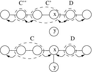
It is very easy to adjust the regular partition, i.e., the regular clusters at level $0$ of the regular multilevel partition. When an edge $e=\{x,y\}$ is inserted, we distinguish between the following cases: 1. the edge $e$ destroys a regular vertex $u$ ; 2. the edge $e$ destroys two regular vertices $u$ and $v$ ; 3. the edge $e$ creates a regular vertex $u$ ; 4. the edges $e$ creates two regular vertices $u$ and $v$ ; 5. the edge $e$ does not change the number of regular vertices. We denote with $C_{u}$ ( $C_{v}$ ) the regular cluster containing the vertex $u$ ( $v$ ). We treat these cases as follows.

1.

If the size of $C_{u}$ is $1$ , then this cluster is deleted. Otherwise if $C_{u}$ is adjacent to a cluster $C$ of size one, remove $u$ from $C_{u}$ and union $C_{u}$ with $C$ .
2.

Apply case 1 to both $C_{u}$ and $C_{v}$ .
3.

Create a new cluster $C_{u}$ only containing $u$ . If $C_{u}$ is adjacent to a cluster $C$ of size one, union $C_{u}$ with $C$ .
4.

Apply case 3, but if both $C_{u}$ and $C_{v}$ are not adjacent to a cluster of size one, then they are unioned together.
5.

Nothing has to be done.

As an example consider the graph depicted in Figure 7. The insertion of edge $\{x,y\}$ destroys the regular vertex $x$ , so we are in case 1. Because $\mathcal{C}^{\prime}$ is adjacent to $\mathcal{C}^{\prime\prime}$ and the size of $\mathcal{C}^{\prime\prime}$ is one, we must union $\mathcal{C}^{\prime}$ and $\mathcal{C}^{\prime\prime}$ together into a new regular cluster $\mathcal{C}$ . The maintenance of the regular partition is completed after adjusting the adjacency information of both $\mathcal{C}$ and $\mathcal{D}$ , as shown in Figure 7.

level $>0$

We assume that the regular partition at level $0$ reflects the insertion of an edge, as discussed above. The number of clusters which have changed, inserted or deleted is at most some constant. We put these clusters in a list $L_{C}$ , $L_{I}$ , and $L_{D}$ according to whether they are changed, inserted or deleted. More specifically, these lists are initialized as follows. Each regular cluster that has been split or combined to form a new regular cluster is inserted in $L_{D}$ , while each new regular cluster is inserted in list $L_{I}$ . The adjacency information is stored with the clusters in $L_{I}$ . For clusters in $L_{D}$ every adjacency information is set to null, except the parent information. For each regular cluster whose set of vertices has not changed but its adjacency information has changed, update the adjacency information and insert it into $L_{C}$ .

We create lists $L_{D}^{\prime}$ , $L_{I}^{\prime}$ , and $L_{C}^{\prime}$ to hold the clusters at the next higher level of the regular multilevel partition. These lists are initially empty.

We first adjust the clusters in the list $L_{D}$ . Every cluster $\mathcal{C}$ in $L_{D}$ is removed from $L_{D}$ , and $\mathcal{C}$ is removed as child from its parent $\mathcal{P}$ (if existing).

•

If $\mathcal{P}$ has no more children, then insert $\mathcal{P}$ in $L_{D}^{\prime}$ .
•

If $\mathcal{P}$ still has a child $\mathcal{C}^{\prime}$ , then if $\mathcal{C}^{\prime}$ is not already in $L_{C}$ or $L_{D}$ , then insert $\mathcal{C}^{\prime}$ into $L_{C}$ .

Next, we search the list $L_{C}$ for clusters that have siblings. Suppose that $\mathcal{C}\in L_{C}$ has a sibling $\mathcal{C}^{\prime}$ and parent $\mathcal{P}$ .

•

If $\mathcal{C}$ and $\mathcal{C}^{\prime}$ are adjacent, then remove $\mathcal{C}$ from the list $L_{C}$ , and remove $\mathcal{C}^{\prime}$ from $L_{C}$ if it is in this list. Insert $\mathcal{P}$ into $L_{C}^{\prime}$ .
•

If $\mathcal{C}$ and $\mathcal{C}^{\prime}$ are not adjacent, then remove $\mathcal{C}$ and $\mathcal{C}^{\prime}$ as children from $\mathcal{P}$ . Remove $\mathcal{C}$ from the list $L_{C}$ , and also remove $\mathcal{C}^{\prime}$ from $L_{C}$ if it is in this list. Insert both $\mathcal{C}$ and $\mathcal{C}^{\prime}$ into $L_{I}$ , and insert $\mathcal{P}$ in $L_{D}^{\prime}$ .

Finally, we treat the remaining clusters in $L_{C}$ and in $L_{I}$ . Let $\mathcal{C}$ be such a cluster. Remove $\mathcal{C}$ from the appropriate list. In what follows, the degree of $\mathcal{C}$ is the number of adjacent clusters.

•

If $\mathcal{C}$ has degree zero, then it is the root of a tree in the regular forest. Insert its parent $\mathcal{P}$ , if existing, in $L_{D}^{\prime}$ .
•
If $\mathcal{C}$ has degree one or two, then we have the following possibilities:
- –
  
  If every adjacent cluster to $\mathcal{C}$ has a sibling, then insert the parent $\mathcal{P}$ of $\mathcal{C}$ into $L_{C}^{\prime}$ in case $\mathcal{P}$ exists. In case $\mathcal{C}$ does not have a parent, create a new parent cluster $\mathcal{P}$ and insert it into $L_{I}^{\prime}$ .
- –
  
  Let $\mathcal{C}^{\prime}$ be a cluster adjacent to $\mathcal{C}$ which has no sibling. Remove $\mathcal{C}^{\prime}$ from the appropriate list, if it is in a list. If both $\mathcal{C}$ and $\mathcal{C}^{\prime}$ have a parent, denoted by $\mathcal{P}$ and $\mathcal{P}^{\prime}$ respectively, then remove $\mathcal{C}$ as child of $\mathcal{P}$ and make it a child of $\mathcal{P}^{\prime}$ . Insert $\mathcal{P}$ into $L_{D}^{\prime}$ , and insert $\mathcal{P^{\prime}}$ into $L_{C}^{\prime}$ . If both $\mathcal{C}$ and $\mathcal{C}^{\prime}$ have no parent, then create a new parent $\mathcal{P}$ of $\mathcal{C}$ and $\mathcal{C}^{\prime}$ , and insert $\mathcal{P}$ into $L_{I}^{\prime}$ . If $\mathcal{C}$ has a parent $\mathcal{P}$ , and $\mathcal{C}^{\prime}$ has no parent, then make $\mathcal{C}^{\prime}$ a child of $\mathcal{P}$ and insert $\mathcal{P}$ into $L_{C}^{\prime}$ . The case that $\mathcal{C}^{\prime}$ has a parent $\mathcal{P}^{\prime}$ , and $\mathcal{C}$ has no parent, is analogous.

When all clusters are removed from $L_{D}$ , $L_{C}$ , and $L_{I}$ , determine and adjust the adjacency information for all clusters in $L_{D}^{\prime}$ , $L_{C}^{\prime}$ , and $L_{I}^{\prime}$ and reset $L_{C}$ to be $L_{C}^{\prime}$ , $L_{C}$ to be $L_{C}^{\prime}$ , and $L_{I}$ to be $L_{I}^{\prime}$ . If no clusters are present in $L_{D}^{\prime}$ , $L_{C}^{\prime}$ or $L_{I}^{\prime}$ , nothing needs to be done and the iteration stops. This completes the description of how to handle the lists $L_{D}$ , $L_{C}$ , and $L_{I}$ .

5.3 Finding a topological edge

Consider that we are in one of the cases 4–6 described in Section 3, where we have to split a topological edge. Let $x$ be the regular vertex at which we have to split the topological edge. We store a pointer from $x$ to the regular cluster $\mathcal{C}_{x}$ in which it is contained. We also store a pointer from each root of a tree $T$ in the regular forest to the topological edge, corresponding to the regular path formed by all vertices in the leaves of $T$ . We find the topological edge which needs to be split by going from $\mathcal{C}_{x}$ to the root of the tree containing $\mathcal{C}_{x}$ . Since the height of the tree is at most $O(\log\ell)$ , where $\ell$ is the current number of edge insertions, we obtain the following.

Proposition 5.1.

Given a regular vertex $x$ , the regular forest returns the topological edge corresponding to the regular path on which this regular vertex lies in $O(\log\ell)$ time.

5.4 Storing weight information

We store weight information in two different places. We define the weight of a regular cluster at level $0$ of size one as zero. Let $\mathcal{C}$ be a cluster at level $0$ of size two, and let $v$ and $w$ be the two regular vertices in $\mathcal{C}$ . Then we define the weight of $\mathcal{C}$ as the weight of the edge $\{v,w\}$ . If a cluster at level $0$ is adjacent to a singular vertex $s$ , then we store the weight of $\{v,s\}$ together with the adjacency information (here, $v$ is the vertex in $\mathcal{C}$ adjacent to $s$ ). If two clusters $\mathcal{C}$ and $\mathcal{C}^{\prime}$ at level $0$ are adjacent, then we store the weight of $\{v,w\}$ together with their adjacency information (here $v\in\mathcal{C}$ and $w\in\mathcal{C}^{\prime}$ and $v$ is adjacent to $w$ ).

The weight of a cluster of size one at level $i>0$ , is defined as the weight of its child at the next lower level. The weight of a cluster of size two at level $i>0$ equals the sum of the weights of its two children and the weight stored with their adjacency information. If two clusters at level $i>0$ are adjacent, we store the weight of the adjacency information of their adjacent children. If a cluster at level $i>0$ is adjacent to a singular node, we store the weight of the adjacency information of its child and the singular node.

5.5 Maintaining weight information

The weight of clusters and the weights stored together with the adjacency information, is updated after each run of the update procedure for the regular multilevel partition, with an extra constant cost. Indeed, both the weights of clusters at level $0$ and the weights stored with the adjacency information, are trivially updated. When we assume that all levels lower than $i$ represent the weight information correctly, the weight information of clusters in $L_{C}$ and $L_{I}$ is trivially updated using the weight information at level $i-1$ .

5.6 Finding the weights

As mentioned above, each root of a regular tree in the regular forest, has a pointer to a unique topological edge. This root has its own weight, as defined above, and is adjacent to two singular vertices. The weight of the topological edge is obtained by summing the weight of the root together with the weights of the adjacency information of the two singular vertices. This is illustrated in Figure 8.

5.7 Complexity Analysis

The complexity of the Topology Tree Algorithm is governed by two things: the maximal height of a single tree in the regular forest, and the amount of work that needs to be done at each level in the maintenance of the regular multilevel partition. We already saw that the height of a single tree is logarithmic in the number of regular vertices on the regular path on which the tree is built. Moreover, Frederickson has proven that in the lists $L_{C}$ , $L_{D}$ , and $L_{I}$ only a constant number of clusters are stored [3]. These lists are updated at most $O(\log\ell)$ times, where $\ell$ is the number of edge insertions, so that the total update time is $O(\log\ell)$ per edge insertion. Hence, we may conclude the following:

Theorem 5.1.

The total time spent on $\ell$ updates by the Topology Tree Algorithm is $O(\ell\log\ell)$ .

6 Experimental Comparison

The Renumbering Algorithm and the Topology Tree Algorithm are very different, but have the same theoretical complexity. Hence, the question arises how they compare experimentally. In this section we try to obtain some insight into this question.

Both algorithms were implemented in C++ using LEDA [9]. We used the GNU g++ compiler version 2.95.2 without any optimization option. Our experiments were performed on a SUN Ultra 10 running at 440 Mhz with 512 MB internal memory. Implementing the Renumbering algorithm was considerably easier than implementing the Topology Tree Algorithm.

We conducted our experiments on three types of inputs. First of all, we extensively studied random inputs, which are random sequences of updates on random graphs. Next, we used two kinds of non-random graph inputs which focus specifically on the merging and the splitting of topological edges. Thereto, we constructed an input sequence which repeatedly merges topological edges, and an input sequence which first creates a very large number of small topological edges, and then splits these edges randomly. Finally, we ran both algorithms on two inputs originating from real data sets.

Methodology

Since the experiments have an element of randomness, we show the results in the form of 95% confidence intervals. For each test, we perform a large number of runs. For each run, we compute the ratio between the total time taken by Topology Tree and that taken by Renumbering. We took the average of these ratios and computed the $95\%$ confidence interval. So, for example, the interval $[1.10,1.15]$ means that Topology Tree was 10 to 15% slower than Renumbering in 95% of the runs in the test.

Random Inputs

The random inputs consist of random graphs that are generated, given the number of vertices and edges. Each run builds a random graph incrementally with the insertions uniformly distributed over the set of edges. We conducted a series of tests for different number of nodes $n$ and number of edges $m$ . For every pair of values for $n$ and $m$ we did $1000$ runs. The results of these experiments are shown in Table 1.

vertices $\backslash$ edges	m=5 000	m=10 000	m=20 000
n=1 000	$[1.10,1.15]$	$[1.03,1.06]$	$[0.97,0.99]$
vertices $\backslash$ edges	m=5 000	m=25 000	m=75 000
n=5000	$[1.25,1.29]$	$[1.01,1.03]$	$[0.96,0.98]$
vertices $\backslash$ edges	m=10 000	m=50 000	m=150 000
n=50 000	$[1.30,1.35]$	$[1.06,1.07]$	$[0.91,0.92]$
vertices $\backslash$ edges	m=10 000	m=100 000	m=300 000
n=100 000	$[1.21,1.23]$	$[0.98,0.99]$	$[0.85,0.86]$

Table 1: 95% confidence intervals on ratio between Topology Tree and Renumbering, from 1000 runs on random inputs.

For small numbers of edge insertions, i.e., when the probability of having many regular vertices is large, we see that the Renumbering Algorithm is faster. However, when the number of edge insertions increases, the Topology Tree Algorithm becomes slightly faster. This is probably due to the fact that the dictionary in the Renumbering Algorithm becomes very large, i.e., there are many short topological edges, and hence it takes longer to search for topological edges.

Non-Random Inputs

The non-random inputs consisted of two types. For the first type, we created a large number of topological edges and then started to merge these edges pairwise. The end result was a very long topological edge. For the second type, we first created a very large number of short regular paths consisting of a single regular vertex, and then started to split these randomly. Each result shown in Table 2 is obtained from $100$ runs.

Merge ( $n=20\,099$ , $m=20\,098$ )	$[3.60,3.74]$
Split ( $n=280\,000$ , $m=200\,000$ )	$[1.15,1.17]$

Table 2: 95% confidence intervals on ratio between Topology Tree and Renumbering, from 100 runs on non-random inputs.

The first type of input was designed in order to reproduce the cases, observed in the random inputs, where Renumbering is much faster than Topology Tree. This is confirmed by the experimental result. Indeed, on this type of inputs, the Topology Tree Algorithm has to maintain large topology trees, which is probably the reason that it is slower.

The second type of input was designed in an attempt to reproduce the cases where Topology Tree is faster than Renumbering. Our attempt failed, however, as the experimental result does not confirm this. Indeed, although the topology trees all have height one, while the dictionary is very large, the Renumbering Algorithm nevertheless still is faster.

Real Data Inputs

We also tested the relative performance of both algorithms with respect to graphs representing real data. We present the results on two data sets:

Hydrography graph: A data set representing the hydrography of Nebraska. This set contains $157\,972$ vertices, of which $96\,636$ are regular.
Railroad graph: A data set representing all railway mainlines, railroad yards, and major sidings in the continental U.S. compiled at a scale $1:100\,000$ . It contains $133\,752$ vertices of which only $14\,261$ are regular. It is available at the U.S. Bureau of Transportation Statistics (www.bts.gov/gis).

The results shown in Table 3 are obtained after performing $100$ experiments. In each experiment, we ran both algorithms in a random way on these data sets. We computed the ratio between the total time the Topology Tree Algorithm needed to perform the test and the total time the Renumbering Algorithm needed to accomplish the same task. We took the average of this ratio and computed the $95\%$ confidence interval.

Hydrography	$[1.62,1.66]$
Railroad	$[0.95,0.96]$

Table 3: 95% confidence intervals on ratio between Topology Tree and Renumbering, from 100 runs on real datasets.

Again, we see that when there are only few, but long, topological edges, the Renumbering Algorithm is faster than the Topology Tree Algorithm. When there are many, short, topological edges, like in the railroad graph, the Topology Tree Algorithm is slightly faster than the Renumbering Algorithm.

In summary, our experimental study shows that when the percentage of regular vertices is high in a graph, then the Renumbering Algorithm is clearly better than the Topological Tree Algorithm, and when the same percentage is low, then the reverse often holds. However, our experimental study did not compare any specific problem solving with and without using topological simplification. Intuitively, the value of topological simplification should increase with the percentage of regular vertices in the graph. Therefore, when the percentage of the regular vertices is high, the Renumbering Algorithm should be not only better than the Topological Tree Algorithm but also yield a significant time saving over problem solving without topological simplification. We expect this to be the most important practical implication of our study for the case when there are only insertions of edges and vertices into the graph. However, when a fully dynamic structure is needed, then the Topological Tree Algorithm should be also advantageous in practice.

Acknowledgement

We would like to thank Bill Waltman for providing us with the hydrography data set.

References

[1] T.H. Cormen, C.E. Leierson, and R.L. Rivest. Introduction to Algorithms. MIT Press, 1990.
[2] M.J. Egenhofer and J.R. Herring, editors. Advances in Spatial Databases, Volume 951 of Lecture Notes in Computer Science, Springer-Verlag, 1995.
[3] G.N. Frederickson. “Data structures for on-line updating of minimal spanning trees”, SIAM J. Comput., Vol 14:781–798, 1985.
[4] G.N. Frederickson. “Ambivalent data structures for dynamic 2-edge-connectivity and $k$ smallest spanning trees”, SIAM J. Comput., Vol 26(2):484–538, 1997.
[5] F. Geerts, B. Kuijpers, and J. Van den Bussche. “Topological canonization of planar spatial data and its incremental maintenance”, In T. Polle, T. Ripke, and K.-D. Schewe, editors, Fundamentals of Information Systems, Kluwer Academic Publishers, 1998, pp 55–68.
[6] G. Italiano. “Dynamic graph algorithms”, In Mikhail J. Atallah, editor, Handbook on Algorithms and Theory of Computation, CRC Press, 1998.
[7] B. Kuijpers, J. Paredaens, and J. Van den Bussche. “Lossless representation of topological spatial data”, In Egenhofer and Herring [2], pages 1–13.
[8] K. Mehlhorn. Data Structures and Algorithms 1: Sorting and Searching, EACTS Monographs on Theoretical Computer Science. Springer-Verlag, 1984.
[9] K. Mehlhorn and S. Näher. “LEDA: A platform for combinatorial and geometric computing”, Comm. of the ACM, Vol 38(1):96–102, 1995.
[10] C.H. Papadimitriou, D. Suciu, and V. Vianu. “Topological queries in spatial databases”, Journal of Computer and System Sciences, Vol 58(1):29–53,1999.
[11] L. Segoufin and V. Vianu. “Querying spatial databases via topological invariants”, Journal of Computer and System Sciences, Vol 61(2):270–301, 2000.
[12] R. Tamassia “On-line planar graph embedding”, Journal of Algorithms, Vol 21:201–239, 1996.
[13] R.E. Tarjan. “Data structures and network algorithms”, In CBMS-NSF Regional Conference Series in Applied Mathematics, Vol 44. SIAM, 1983.
[14] M.F. Worboys. GIS: A Computing Perspective, Taylor&Francis, 1995.

On-line topological simplification of weighted graphs