The Aligned-Coordinated Geographical Routing for Multihop Wireless Networks
Abstract
The stateless, low overhead and distributed nature of the Geographic routing protocols attract a lot of research attentions recently. Since the geographic routing would face void problems, leading to complementary routing such as perimeter routing which degrades the performance of geographic routing, most research works are focus on optimizing this complementary part of geographic routing to improve it. The greedy forwarding part of geographic routing provides an optimal routing performance in terms of path stretch. If the geographic routing could adapt the greedy forwarding more, its performance would be enhanced much more than to optimize the complementary routing such as perimeter routings. Our work is the first time to do so. The aligned physical coordinate is used to do the greedy forwarding routing decision which would lead more greedy forwarding. We evaluate our design to most geographic routing protocols, showing it helps much and maintain the stateless nature of geographic routing.
1 Introduction
2 Related work
3 Connectivity Sensitive Alignment
3.1 Intuition
As our observation, in a wireless network with random deployment, the 2 data forwarding pathes in 2 directions between a pair of nodes are mostly not through the same nodes, using GPSR as routing protocol. And mostly, if in one direction, the path consists of both greedy forwarding phase and perimeter routing phase, in the other direction with different set of forwarding nodes, the path may keep just in greedy forwarding as an optimal one in term of number of hops (the shortest path).


The figure 1 shows a practice example of our observation. From node to , data packet would be forwarded to node first, according to greedy principle; then it meets a void, starting a perimeter routing phase; after reaching node , it comes back to greedy forwarding again, until arriving at destination , shown in figure 1(a).
Meanwhile, if a data packet is being forwarded from node to , the situation would be very different. It would be always forwarded greedily, through a shorter path with 2 hops less than the reverse one, as shown in figure 1(b).
Based on this observation, we questioned: is it possible to find a way to reduce, or even extinct, the ratio of this situation so as to increase the greedy ratio of the routing, resulting in an enhancement of the routing performance.
Conservation routing protocols, such as DSR or AODV, are based on broadcast and flooding. Before forwarding data packets, the routing protocol would construct a shortest path between the source and destination, with an overview of the whole network topology obtained through the flooding. The overhead is high due to the flooding nature. On the other hand, the stateless geogrpahic routing protocols such as GPSR is based on only the location information of all one-hop neighbors, leading to a lower overhead. The drawback is the void problem where the greedy forwarding would fail, leading to sub-optimal routing pathes.
In GPSR, the void may not be known before a packet reaches it. The reason comes from the stateless nature of it, lack of overview of not the whole network, but even 2 or more hops away. If before facing a void, the routing protocol can find a way to predict the void, and detour earlier, a perimeter routing phase is possible to be avoided. Even worse, the one-hop information is not fully utilized. Only the location information of them is used for routing. Intuitively, if the connection information is used for routing as well, it would help.
3.2 Aligned coordinates of physical location
The connectivity of a node is decided by all its neighbors, the neighbors of neighbors, and so on. In this section, we try to align the physical location of a node to all its neighbors, with the connectivity information.
The aligned coordinates of a node, is a vector whose direction and distance are decided by its neighborhood. Or say, the direction is from its physical location to the average position of all its neighbors, with a distance scaler as the standard deviation of the distances between all its neighbors and itself.
Suppose the location (physical coordinates) of node is , the set of all its neighbor nodes is , and is the location of the neighbor node . The denotes the distance between node and , and denotes the number of nodes in . Then the average position of all neighbor nodes of is
| (1) |
The average distance between node and all its neighbors is
| (2) |
The distance between the aligned location and node meets the standard deviation as
| (3) |
So the aligned location of node is
| (4) |
where the is the normalized vector of .
As we can see, the alignment reflects the neighborhood connectivity of a node with the standard deviation as the stretch. The average location of all neighbors indicates to which direction, the node would have a higher chance to find a neighbor, or next hop in routing. The stretch of it shows how much the chance is.
The depth of the alignment is the number of hops in which the neighboring information is used for aligning. For example, if only the physical location information of all one-hop neighbors is used for aligning of any node, the alignment depth of this node is 1. If the aligned location information with depth of all one-hop neighbors is used, the alignment depth of this node would be .

Xc is the average of neighbor nodes of X, and X’ is aligned location of node X
The figure 2 shows an example of how to align the physical location of a node into the aligned coordinates. According to equation 1, we have the average position of all neighbor nodes of
And the average distance between and its neighbor s is
and the deviation is
So we have the aligned coordinates with depth 1 of node as
3.3 Aligned Coordinates help Routing
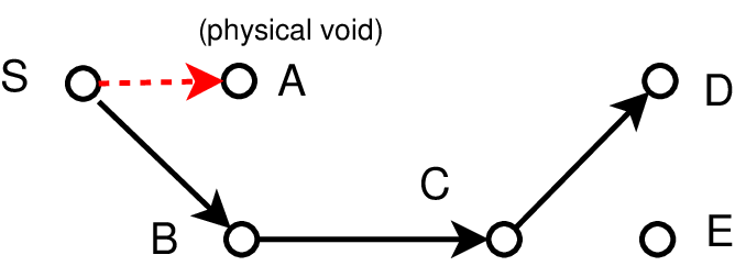
The dot line is the greedy forwarding path on physical coordinates; The concrete line is the greedy forwarding path on aligned coordinates.
The figure 3 shows a 6-node network. Node is the data source and the is the destination. Suppose the radio range of the nodes is 1.5 unit. All other information is listed in table 1.
| X | |||||
|---|---|---|---|---|---|
| S | A, B | ||||
| A | S, B | ||||
| B | S, A, C | ||||
| C | B, E | ||||
| D | C, E | - | - | ||
| E | C, D |
Since in a multihop wireless network, the alignment information of several hop away may be difficult to obtained. Even obtained, it may be stale quickly due to many reasons such as node mobility. To maintain the stateless nature of geographic routing protocols, only the un-aligned physical location information of the destination would be used for distance calculating. So in stead of using , is adapted.
As we can see, without alignment, at first data packet would be forwarded greedily from node to node . Since , it reaches a void, which may trigger a permeter routing. With alignment, , node would forward packet greedily to , then , and finally .