Outlier Robust ICP for Minimizing Fractional RMSD
Abstract
We describe a variation of the iterative closest point (ICP) algorithm for aligning two point sets under a set of transformations. Our algorithm is superior to previous algorithms because (1) in determining the optimal alignment, it identifies and discards likely outliers in a statistically robust manner, and (2) it is guaranteed to converge to a locally optimal solution. To this end, we formalize a new distance measure, fractional root mean squared distance (frmsd), which incorporates the fraction of inliers into the distance function. We lay out a specific implementation, but our framework can easily incorporate most techniques and heuristics from modern registration algorithms. We experimentally validate our algorithm against previous techniques on 2 and 3 dimensional data exposed to a variety of outlier types.
1 Introduction
Aligning an input data set to a model data set is fundamental to many important problems such as scanned model reconstruction [16], structural biochemistry [25], and medical imaging [12]. The input data and the model data are typically given as a set of points. A point set may arise from laser scans of a 3D or 2D model, coordinates of atoms in a protein, positions of a lesions from a medical patient, or some other sparse representation of data. However, the relative positions of these point sets is not known, making the task of registering them nontrivial.
A popular approach to solving this problem is known as the iterative closest point (ICP) algorithm [1, 3] which alternates between finding the optimal correspondence between points, and finding the optimal transformation of one point set onto the other. As both steps reduce the distance between the point sets, this process converges, but only to a local minimum. The effectiveness, simplicity, and generality of this algorithm has led to many variations [26, 20, 19, 4, 5, 10, 18, 25]. For instance, the set of legal transformations can be just translations, all rigid motions, or all affine transformations. Other versions replace the optimal correspondence between points by aligning each data point to the closest point on an implicit surface of the model data [3]. Or the traditional squared distance can be replaced with a more efficient and stable approximation to the squared distance function [15]. A now slightly outdated, but excellent survey [20] evaluates many of these techniques.
Yet, because ICP only converges to a local minimum, there has been considerable work on expanding and stabilizing the funnel of convergence—the set of initial positions for which ICP converges to the correct local minimum. Others have attempted to solve the global registration problem [17, 11], where for any initial alignment they attempt to find the optimal alignment between two point sets. This is often done in two steps. First find a rough global alignment by corresponding certain distinguishable feature points. Second refine the alignment with ICP.
However, all of these algorithms are vulnerable to point sets with outliers. Outliers may result from:
- •
measurement error,
- •
spurious data that was ignored or missed in the model,
- •
partial matches because the point sets represent overlapping, but not identical pieces of the same object,
- •
interesting changes in the underlying object between time steps or among comparable objects.
In short, outliers are unavoidable. Because ICP will find correspondences for all points, and then find the optimal transformation for the entire point set, the outliers will skew the alignment. Many heuristics have been suggested [5, 4] including only aligning points within a set threshold [26, 22], but most of these techniques are not guaranteed to converge, and thus can possibly go into an infinite loop, or require an expensive check to prevent this. If the fraction of points which are outliers is known, then Trimmed ICP [4] can be used to find the optimal alignment of the most relevant fraction of points. This algorithm is explained in detail in Section 3.1. However, this fraction is rarely known a priori. If an alignment is given then RANSAC type methods [9, 2] can be used to determine a good threshold for determining these outliers. There are also many ad hoc solutions to this problem. However, if the outliers are excluded from the data set in a particular alignment, then the alignment is no longer optimal, since those outliers which were removed influenced how the points were initially aligned.
1.1 Our Contributions
Our solution to these problems is to incorporate the fraction of points which are outliers into the problem statement and into the function being optimized. To this end, this paper makes the following contributions:
- •
We formalize a new distance measure between point sets which accounts for outliers: frmsd. This definition extends the standard rmsd to account for outliers (Section 2).
- •
- •
- •
Finally, we empirically demonstrate that Fractional ICP identifies the correct alignment while simultaneously determining the outliers on several data sets (Section 7).
2 Fractional RMS Distance
Consider two point sets . The goal of this paper is to align an input data set to a model data set under some class of transformations, . These may include rotations, translations, scaling, or all affine transforms. We assume that these point sets are quite similar and there exists a strong correspondence between most points in the data. There may, however, be outliers, points in either set which are not close to any point in the other set. Our goal is to define and minimize over a set of transformations a relevant distance between these two point sets. To aid in this, we define a matching function , which unless defined otherwise or given as a parameter, simply matches each point of to the closest point in .
Definition 1.
[rmsd ] The root mean squared distance (or rmsd) between two point sets , for a given matching is the square root of the average squared distance between matched points:
When convenient we sometimes write , letting match every point in to the closest point in .
Problem 2.1.
[minimizing rmsd ] Given a model point set and an input data point set where , compute the transformation to minimize :
Problem 2.1 is algorithmically difficult because as varies, so does the optimal matching . Also, rmsd is quite susceptible to outliers because the squared distance gives a large weight to outliers. To counteract this, a specific fraction of points from can be used in the alignment and in the distance measure between the point sets. These points can be chosen to solve Problem 2.1 by selecting the points which have the smallest residual distance . Let . But what fraction of points should be used? We can always make by setting and aligning any single point exactly to another point. So rmsd by itself is no longer a viable measure. For this reason, we propose a new distance measure.
Definition 2.
[frmsd ] The fractional root mean squared distance (or frmsd) is defined as follows:
We will empirically and mathematically justify a value of in Section 7.4 and Section 6. Again, it is sometimes convenient to let because can still be determined by and . This leads to a new, more relevant problem.
Problem 2.2.
[minimize frmsd ] Given a model point set and an input data point set where , compute the transformation and fraction to minimize :
Intuitively, the term serves to balance the rmsd term. goes to as goes to , while the rmsd goes to as goes to . frmsd, unlike rmsd over any fraction of the data points, cannot equal unless some fraction of points align exactly. Of course, one point can always align exactly to another point in the other subset, so in the implementation we restrict that , although this case is degenerate and almost never happens in practice. Some arbitrary nonzero minimum value of can be set as desired.
3 Algorithms
In this section we describe algorithms to solve Problem 2.2.
3.1 Trimmed ICP
The Trimmed ICP algorithm 1 assumes to be given and computes a transformation of a point set to minimize rmsd between and a model point set . When , this is the ICP algorithm [1]. The algorithm iterates between computing the optimal matching and the optimal transform over the closest points. This algorithm has been shown [4] to converge to a local minimum of over all rotations, translations, and matchings.
In practice, the comparison on line 8 of Algorithm 1, ), can be replaced by checking whether the value decreases by less than some threshold at each step. TrICP, however, does not completely solve Problem 2.2; is not minimized with respect to . It has been suggested [4] to run TrICP for several values of . In fact, those same authors hypothesize that the values returned from TrICP are convex in , allowing them to perform a golden ratio search technique to avoid checking all values of . This hypothesis is easily shown to be false. Also this technique fails to guarantee that the solution is a local minimum in the space of all transformations, matchings, and fractions. The value attained by TrICP depends on the initial position of and . Thus, for the transformation calculated by TrICP, potentially another fraction can give a smaller value of or of .
3.2 Fractional ICP
A simple modification of TrICP, shown in Algorithm 2, will actually provide the desired local minimum. We refer to this algorithm as Fractional ICP or FICP.
Again, in practice, the comparison on line 10 of Algorithm 2 can be replaced be checking whether the value decreases by less than some threshold at each step.
3.3 Implementation
To implement TrICP we need 3 operations: computing the matching, computing the subset , and computing the transformation. To implement FICP we need the additional step of computing the fraction.
3.3.1 Computing the Matching
For each point we need to find its closest point . Since is fixed through the algorithm, we can precompute a hierarchical data structure which can quickly return the nearest neighbor. We implemented a -tree, at a one-time, initial cost of . The nearest neighbor can be returned in time. This operation is required for each point in . So the matching can be computed in . This is in general the most time consuming step of the algorithm.
3.3.2 Computing the Subset
The set is defined by the points with the smallest residual distances . This observation implies the following algorithm. Compute and sort all residual distances and let be the points with the smallest residual distances. The runtime is bounded by the sorting which takes time.
3.3.3 Computing the Transformation
The set of allowable transformations, , may include rotations, translations, and scalings. Or it may be as general as all affine transformations. When we consider rotations, translations, and scalings, Problem 2.1 is written:
For a fixed matching, , this is known as the absolute orientation problem, and can be solved exactly [14] in time. When , this can be solved in time [24]. There are actually 4 distinct algorithms—one using rotation matrices and the SVD [13], one using rotation matrices and the eigenvalue decomposition [21], one using unit quaternions [8], and one using dual number quaternions [24]—but all are in practice approximately equivalent in run time [6]. We use the simplest technique [13] which reduces the solution to computing an SVD.
When is the set of all affine transformations, Problem 2.1 is written:
where is an affine transformation. This reduces to a generic least squares problem that can be solved with a matrix inversion.
3.3.4 Computing the Fraction
There are only fractions which we need to consider. Consider the sorted order of the point set by each point’s residual distance . Each prefix of this ordering represents a distinct fraction. If we maintain the value for each we can compute in constant time for a given fraction . We can also update to a point set of size in constant time by adding the next point in the sorted order to . If the th prefix yields the smallest value of frmsd, then is set to . So this computation takes time.
4 Convergence of Algorithm
In this section we show that Algorithm 2 converges to a local minimum of over the space of all transformations, matchings, and fractions of points used in the matching. This is a local minimum in a sense that if all but one of transformations, matchings, or fractions is fixed, then the value of the remaining variable cannot be changed to decrease the value of .
Theorem 4.1.
For any two points sets , Algorithm 2 converges to a local minimum of over .
Proof 4.2.
Algorithm 2 only changes the value of when computing the optimal transformation (line 7), computing the optimal matching (line 8), or computing the optimal fraction (line 9). None of these steps can increase the value of , because staying at the current value would retain the value of , but each can potentially decrease it. (When two possible values of degenerately produce the same value of , we consistently choose the smaller one according to some consistent, but arbitrary ordering.)
FICP terminates only when and . The optimal transformation computed at iteration (line 7) is a function of the matching of the points and which points are included, which is determined by . Thus, the transformation will only change in iteration if or change from or , respectively. If and then FICP will terminate, and will be a local minimum. If it were not, then either or would have changed in the last iteration, and would have decreased or stayed the same in the th iteration.
Furthermore, FICP terminates in a finite number of iterations, because there are possible values of and possible values of , and the algorithm can never be at any of these locations twice.
In practice the convergence is much faster than the upper bound of steps. ICP has recently [7] been shown to require iterations for certain adversarial inputs; however, these rarely occur in practice. Furthermore, Pottmann et. al. [19], have shown that ICP has linear convergence when it is close to the optimal solution and a point-to-point matching is used. However, ICP has quadratic convergence when using a point-to-surface or other similar matching criterion as described in [19] or [18]. The lower bounds clearly hold for TrICP. The upper bounds, in terms of convergence rates, intuitively hold, but the reduction seems a little more complicated. Such a proof is outside the scope of this paper.
5 Data Generation Model
In order to formalize the expected mathematical properties of the frmsd measure and the FICP algorithm, we now state some fairly general assumptions about the input data. All data on which FICP is used need not these exact properties, but we hope that these properties are general enough that whatever differences exist in the alternative data will not significantly affect the following analysis and the resulting conclusions.
Since data come from a measurement process that might generate spurious measurements as well as miss valid ones, we do not require every data point to have a corresponding model point, or viceversa. Specifically, we assume that data points are generated from model points by the following abstract procedure:
- 1.
Generate a set of model points that will have corresponding data points (the subscript stands for “inlier”).
- 2.
For every model point , let
be the corresponding data point, where is a transformation in the set and is isotropic Gaussian noise with standard deviation . The set of data points corresponding to is denoted as .
- 3.
Generate a random set of data outliers.
- 4.
Generate a random set of model outliers out of a spatial Poisson process.
We let and . Let be the fraction of data inliers relative to all data points. The detailed spatial statistics of data outliers are irrelevant to our analysis. The Poisson process for model outliers is a minimally informative prior. We let the density of this process be points per unit volume.
The probability density of the squared magnitude of the correspondence noise is a chi square density in dimensions:
where
is the gamma function. In particular,
The expected number of model outliers in a region of space with volume is equal to .
Suppose now that the correct geometric transformation is applied to data point to obtain the transformed data point
(see step 2 in the data generation model above).
If and correspond, their distance statistics are chi square. If and do not correspond, the situation is more complex: Either point (or both) could be an outlier, or they could be non-corresponding inliers. We do not know the distance statistics for model inliers. In the remainder of this section, we assume that the probability that a data inlier is nearest to a non-corresponding model inlier is negligible. Under this assumption, the probability density of the distance from to the nearest outlier, given that model outliers are from a spatial Poisson process with density points per unit volume, can be shown to be
where
is the surface of the unit sphere in dimensions and is the gamma function. The function is known as the Weibull density with shape parameter (equal to the dimension of space) and scale parameter
So far we have not specified the units of measure. Since is a distance and is a distance raised to power (density per unit volume), the parameter is dimensionless. As long as and are properly scaled to each other, the analysis that follows is independent of .
6 The Value of
In this Section we justify a particular choice for the value of used in the definition of the fractional root mean squared distance (frmsd).
As shown in Section 3.3.4, the FICP algorithm selects a fraction of data-model matches in increasing order of their residual distances between data points and their nearest model points . Because of this, choosing a fraction is equivalent to choosing a maximum allowed value for the residual distance . Since we would like the FICP algorithm to favor inliers over outliers, it makes sense to require to be defined in such a way that data points that are away from a model point are equally likely to be inliers as they are to be outliers. Let us call such a value of the critical distance. We then ask the following question: Is there a value of in the definition of the frmsd for which the value of chosen by the FICP algorithm corresponds to the critical distance?
To answer this question, we first express as a function of the model parameters (Section 6.1), and determine the function that relates an arbitrary distance to the corresponding fraction (Section 6.2). We then write an estimate of the frmsd under an ergodicity assumption (Section 6.3). This estimate is itself a function of , and therefore of . The FICP algorithm maximizes the frmsd with respect to , that is, finds a zero for the derivative of the frmsd with respect to . Setting the value of where this zero is achieved to yields an equation for , whose solution set justifies our choice for this parameter (Section 6.4).
Our analysis holds for outlier densities that are below a certain value , which is inversely proportional to the standard deviation of the noise that affects the data points. If outliers exceed this density, then matching data and model points based on minimum distance is too unreliable to yield good results.
6.1 The Critical Distance
Define so that a data and a model point at distance from each other are equally likely to correspond to each other as they are not to. This section derives an expression for as a function of the standard deviation of the correspondence noise, the density of the spatial Poisson process that generates unmatched points, and the dimension of space.
The volume of a sphere of radius in dimensions is
where was defined in Section 5. The volume of the shell between radii and is
This approximation is asymptotically exact as .
The probability mass in the same shell for an isotropic Gaussian distribution with zero mean and standard deviation is
as (the term derives from the Jacobian of the transformation , since the density is defined for the square of a distance) .
Assume that the center of the shell above is at the transformed data point defined in Section 5. As explained in Section 5, if and correspond, their distance statistics are chi squared, and the likelihood of a particular radius is . Otherwise, the distance statistics are approximately described by a spatial Poisson process with density . Then, the critical distance is determined by the equation
that is,
which can be simplified to the following:
| (1) |
The left-hand side of equation (1) is strictly positive and monotonically decreasing in and the right-hand side is constant, so the equation admits a solution if and only if
If the outliers exceed this maximum density , the critical distance shrinks to zero: any model point around any given data point is more likely to be an outlier than it is to be the model point corresponding to . Of course, when there are no model outliers () the concept of critical distance loses its significance.
Equation (1) can be solved for to yield the desired value of as a function of the model parameters:
The critical distance normalized by and expressed as a function of is
This function is independent of all model parameters and is plotted in Figure 1.

6.2 Relationship between and
As explained earlier, to every fraction of data points considered by the FICP algorithm there corresponds a maximum distance , in the sense that data-model point pairs have distance at most . Consider a particular data point and its transformed version . If the data generation process is ergodic, the fraction equals the probability that the nearest model point to a point selected at random from the transformed data set is at most away.
With probability , the data point has a corresponding model point (inlier). In this event, if is the distance from this model point and is the distance from the nearest model outlier point, the complement of the cumulative probability function of the distance to the nearest model point (either inlier or outlier) is
where and are respectively the probability that the matching model point and the nearest model outlier are at most units away from . From Section 5, these probabilities are as follows:
and
Then, if has a corresponding model point, the density of its distance from the nearest model point is
With probability , the data point is instead an outlier. Then, it has no corresponding model point, so the probability that the nearest model point is at most units away is simply . In summary, the probability density of the distance between a data point and its nearest model point is
and the average fraction of model points within units from a data point is
The derivative of with respect to is .
6.3 Ergodic Estimate of the frmsd
An estimate of the fractional root mean squared distance (frmsd) can be obtained by assuming ergodically that the sample moment included in the definition of frmsd is close to the corresponding statistical moment:
This assumption requires both ergodicity and a sufficient number of data points that are close enough to the model points. We can then write
6.4 Stationary Point of the frmsd Estimate
At the minimum of , the derivative of with respect to is zero. Differentiation of the expression at the end of Section 6.3 yields
Since
the last addend simplifies to , and
Zeroing this derivative and setting and yields the following equation for :
Figure 2 plots the values of in two and three dimensions as a function of the relative model outlier density and for various values of the data inlier fraction .
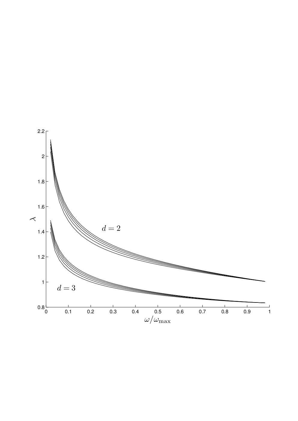
Since the noise standard deviation acts merely as an overall scale factor, these plots do not depend on . It is apparent from the figure that depends weakly on the fraction of data inliers. The knees of the plots are at about and for and dimensions, respectively, corresponding to . These knee values are selected as general-purpose values for the definition of frmsd in two and three dimensions.
7 Experiments
The main advantage of FICP over other variants of ICP is that it automatically determines the outlier set via a fraction and reaches a optimum in terms of the correspondence, the transformation, and the fraction of outliers. In doing so, it takes less time than algorithms which have no guarantees, despite searching a larger parameter space. We also demonstrate that the radius of convergence for FICP is expanded as compared to TrICP.
Finally, we deal empirically with the issue of the parameter used in the definition of frmsd. We observe that frmsd is robust to the choice of within a broad range. However the radius of convergence and efficiency of FICP is improved when is set to a slightly higher values than those determined optimal for identifying outliers in Section 6. Intuitively, a smaller value of is more likely to classify correct correspondences as outliers when the alignment is not close, and thus get stuck in local minimum. For higher values of these types of local minimum seem less prevalent. So for all performance studies we set , unless otherwise specified. For this value FICP has an expanded radius of convergence and tends to find very similar alignments as when is set according to the analysis in Section 6. After converging, we recommend setting for or for to identify outliers more agressively. This final phase should take very few additional iterations of the algorithm, since, as we demonstrate, moderately modifying the value of has small effects on the frmsd and values returned.
7.1 Data Sets
We perform many tests on the SQUID fish contour database [23] from the University of Surrey, UK. This database has 1100 2D contours of fish and each contour has 500 to 3000 points. The size of this data set allows us to average results over a very large set of experiments. We do not know of any 3D database even close to this size, and it has been previously used to evaluate TrICP [4].
We also perform some experiments on a limited number of 3D models. In particular we use the bunny and the happy Buddha data set from the Stanford 3D Scanning Repository.
We synthetically introduce outliers into the data sets in 3 ways. We always begin by creating two copies and , to represent the model and the input data, of the particular data set. A parameter fraction of the final set are left undisturbed as data inliers.
- •
Occlusion: We randomly choose a ball and remove all of the points from within . This test represents cases where the model set is only partially observed because of occlusions, where there are two overlapping views of the same object that do not exactly align, or where the input data has grown since the model was formed. An example is shown in Figure 3.
- •
Deformation: We randomly choose a ball and shift randomly the points . This represents the case where is deformed slightly between time steps. See Figure 4.
- •
New data: We add a set of points to . These points are placed uniformly at random within a bounding box of . This represents outliers caused by some sort of data retrieval noise or from spurious or new data. See Figure 5.
Finally, we always introduce some further noise in the models. For each point , we create a random vector distributed according to a Gaussian distribution with standard deviation , and we add to .


We perform many tests on synthetic data because we then know that a good match exists and it is thus easy to quantify the performance on our algorithm.
Additionally, we perform tests on real scanned data. We align pairs of scanned images of the dragon model from the Stanford 3D Scanning Repository from views or apart. Because the different views observe different portions of the model, there are many points which have no good alignment in both the model and data set. These are outliers.
7.2 Performance
For each synthetic data set and type of outliers described above, we perform the following set of tests. We first rotate by degrees where is from the set . The axis of rotation is chosen randomly for the 3D data. We then run ICP, TrICP searching for with the golden rectangle search, and FICP, minimizing over all rigid motions. We report the total number of iterations of each, the run time, and the final values of rmsd, frmsd, and . We vary the input so that is either . We expect that optimally should be near since in our data is small compared to . All experiments were performed on a 3 GHz Pentium IV processor with 1 Gb SD-RAM.
We show in Table 1 the average performance of all algorithms on the entire SQUID data set where points are removed from , giving occlusion outliers with . Table 2 shows the same where is given deformation outliers with . Table 3 shows where is given new data outliers with . TrICP and FICP return similar values of rmsd and frmsd on average while also determining reasonable values for . However, FICP is about faster than TrICP using the golden ratio search.
| Algorithm | time (s) | # iterations | rmsd | frmsd | f | |
|---|---|---|---|---|---|---|
| ICP | .75 | 0.335 | 24.5 | 9.454 | 9.454 | 1.000 |
| TrICP | .75 | 1.356 | 117.9 | 0.217 | 0.541 | 0.744 |
| FICP | .75 | 0.178 | 13.6 | 0.178 | 0.424 | 0.749 |
| ICP | .88 | 0.21 | 21.4 | 4.079 | 4.079 | 1.000 |
| TrICP | .88 | 1.032 | 107.5 | 0.218 | 0.364 | 0.784 |
| FICP | .88 | 0.136 | 12.3 | 0.175 | 0.258 | 0.878 |
| ICP | .95 | 0.137 | 15.9 | 1.338 | 1.338 | 1.000 |
| TrICP | .95 | 0.913 | 102.4 | 0.197 | 0.261 | 0.904 |
| FICP | .95 | 0.123 | 12.0 | 0.175 | 0.205 | 0.949 |
| Algorithm | time (s) | # iterations | rmsd | frmsd | f | |
|---|---|---|---|---|---|---|
| ICP | .75 | 0.263 | 28.9 | 1.074 | 1.074 | 1.000 |
| TrICP | .75 | 1.103 | 114.8 | 0.213 | 0.404 | 0.803 |
| FICP | .75 | 0.191 | 18.1 | 0.231 | 0.402 | 0.810 |
| ICP | .88 | 0.215 | 24.4 | 0.829 | 0.829 | 1.000 |
| TrICP | .88 | 1.065 | 112.8 | 0.213 | 0.335 | 0.827 |
| FICP | .88 | 0.148 | 14.2 | 0.178 | 0.241 | 0.903 |
| ICP | .95 | 0.168 | 19.6 | 0.569 | 0.569 | 1.000 |
| TrICP | .95 | 1.020 | 111.6 | 0.203 | 0.281 | 0.900 |
| FICP | .95 | 0.138 | 13.3 | 0.174 | 0.197 | 0.959 |
| Algorithm | time (s) | # iterations | rmsd | frmsd | f | |
|---|---|---|---|---|---|---|
| ICP | .75 | 0.461 | 26.7 | 5.820 | 5.820 | 1.000 |
| TrICP | .75 | 1.578 | 92.9 | 0.176 | 0.399 | 0.768 |
| FICP | .75 | 0.264 | 13.7 | 0.175 | 0.388 | 0.766 |
| ICP | .88 | 0.286 | 23.7 | 4.061 | 4.061 | 1.000 |
| TrICP | .88 | 1.351 | 108.0 | 0.202 | 0.309 | 0.831 |
| FICP | .88 | 0.183 | 13.1 | 0.172 | 0.246 | 0.888 |
| ICP | .95 | 0.192 | 19.5 | 2.626 | 2.626 | 1.000 |
| TrICP | .95 | 1.135 | 108.3 | 0.205 | 0.295 | 0.893 |
| FICP | .95 | 0.148 | 12.6 | 0.171 | 0.197 | 0.953 |
The values when deformation outliers are introduced are noticeably larger than because some of the shifted points happen to lie very near model points when the two data sets are properly aligned. These points might as well be inliers. This phenomenon is less common for the other types of synthetically generated outliers.
We also ran the same experiments with the same algorithms on the bunny (35,947 points) and happy Buddha (144,647 points) data from the Stanford 3D scanning repository. We report the results on the bunny data set in Table 4 and for the happy Buddha data set in Table 5 where deformation outliers are applied to and then is randomly rotated by . The numbers are the the results of averages over random rotations.
| Algorithm | time (s) | # iterations | rmsd | frmsd | f | |
|---|---|---|---|---|---|---|
| ICP | .75 | 60.1 | 78.8 | 0.66682 | 0.66682 | 1.000 |
| TrICP | .75 | 136.5 | 172.2 | 0.00523 | 0.01239 | 0.750 |
| FICP | .75 | 16.5 | 17.3 | 0.00522 | 0.01237 | 0.750 |
| ICP | .88 | 29.6 | 48.0 | 0.45303 | 0.45303 | 1.000 |
| TrICP | .88 | 147.1 | 224.3 | 0.00522 | 0.00767 | 0.880 |
| FICP | .88 | 13.7 | 15.9 | 0.00522 | 0.00767 | 0.880 |
| ICP | .95 | 13.8 | 31.3 | 0.37207 | 0.37207 | 1.000 |
| TrICP | .95 | 77.6 | 162.8 | 0.00523 | 0.00610 | 0.950 |
| FICP | .95 | 8.0 | 14.2 | 0.00523 | 0.00610 | 0.950 |
| Algorithm | time (s) | # iterations | rmsd | frmsd | f | |
|---|---|---|---|---|---|---|
| ICP | .75 | 430.8 | 66.6 | 0.56145 | 0.56146 | 1.000 |
| TrICP | .75 | 727.3 | 101.0 | 0.00123 | 0.00291 | 0.750 |
| FICP | .75 | 139.7 | 15.6 | 0.00119 | 0.00282 | 0.750 |
| ICP | .88 | 109.2 | 28.2 | 0.29745 | 0.29745 | 1.000 |
| TrICP | .88 | 485.4 | 120.5 | 0.00120 | 0.00177 | 0.880 |
| FICP | .88 | 81.4 | 15.7 | 0.00119 | 0.00174 | 0.880 |
| ICP | .95 | 126.1 | 45.4 | 0.29351 | 0.29351 | 1.000 |
| TrICP | .95 | 405.2 | 123.7 | 0.00120 | 0.00141 | 0.950 |
| FICP | .95 | 66.3 | 14.6 | 0.00119 | 0.00139 | 0.950 |
Observe in Figure 6 how in the alignment of the bunny data set, the non-deformed points (red points on back side, blue points are not visible because they lie exactly behind the red points) are aligned almost exactly by the FICP algorithm while the deformed points (shifted from visible blue points in front) are ignored. Such an alignment allows one to easily identify the portion of the data which has been deformed, and by how much it has been deformed. Without a proper registration to the model the unaligned points have no point of comparison to gauge their deformation. The alignment is skewed when ICP is used and it is not helpful in determining which points are deformed.


7.3 Funnel of Convergence
We calculate the percentage of cases from the SQUID data set that converge to an frmsd value within and value within of the alignment between the same sets with no initial rotation. Table 6 shows the results when New Data outliers with are added to the data set . The results for the other types of noise are simlar. For 3D data sets we chose proportionally smaller, so these convergence rates are all slightly larger. Note that FICP with performs much better than when .
| Algorithm | |||||
|---|---|---|---|---|---|
| ICP | - | 0.999 | 0.997 | 0.994 | 0.962 |
| TrICP | 3 | 0.875 | 0.870 | 0.853 | 0.816 |
| FICP | 3 | 0.952 | 0.945 | 0.909 | 0.875 |
| FICP | 1.3 | 0.857 | 0.473 | 0.141 | 0.060 |
ICP has a larger radius of convergence than FICP, because it searches a much smaller parameter space. FICP has a larger radius of convergence than TrICP even though they search the same parameter space.
7.4 Validating
We empirically justify that frmsd is not sensitive to the choice of . We run FICP with set to . We plot the averaged results on the SQUID data set when Occlusion noise is added with and is initially rotated and in Table 7 and Table 8, respectively. Altering does not dramatically affect the converged solution, but can affect the radius of convergence. The output is similar for different types of noise. On 3D data, FICP performs slightly better than 2D data for smaller .
| Algorithm | time (s) | # iterations | rmsd | frmsd | f | |
|---|---|---|---|---|---|---|
| FICP | 1 | 0.142 | 10.38 | 0.158 | 0.225 | 0.701 |
| FICP | 1.3 | 0.069 | 3.81 | 0.170 | 0.248 | 0.749 |
| FICP | 2 | 0.059 | 3.06 | 0.170 | 0.303 | 0.750 |
| FICP | 3 | 0.061 | 3.17 | 0.170 | 0.404 | 0.750 |
| FICP | 4 | 0.062 | 3.21 | 0.171 | 0.538 | 0.751 |
| FICP | 5 | 0.063 | 3.30 | 0.172 | 0.717 | 0.751 |
| Algorithm | time (s) | # iterations | rmsd | frmsd | f | |
|---|---|---|---|---|---|---|
| FICP | 1 | 0.733 | 37.23 | 0.298 | 1.503 | 0.274 |
| FICP | 1.3 | 0.488 | 36.44 | 0.219 | 0.563 | 0.660 |
| FICP | 2 | 0.244 | 17.00 | 0.176 | 0.329 | 0.740 |
| FICP | 3 | 0.198 | 13.59 | 0.178 | 0.424 | 0.749 |
| FICP | 4 | 0.194 | 13.28 | 0.184 | 0.570 | 0.751 |
| FICP | 5 | 0.200 | 13.66 | 0.299 | 0.875 | 0.756 |
7.5 Aligning Scanned Model Data
Finally, we perform experiments aligning real scanned range maps from 3D models. We consider aligning two scans from the Stanford 3D scanning repository of the dragon model. We take scans from the dragonStandRight data set and we align consecutive scans ( apart), as seen in Table 9, and next-to-consecutive scans ( apart), as seen in Table 10. We first rotate the later scan by or to bring the scans into the approximately correct alignment. We then align them with ICP, TrICP, and FICP.
| Algorithm | angle1 | angle2 | time (s) | # iterations | rmsd | frmsd | f |
|---|---|---|---|---|---|---|---|
| ICP | 336 | 0 | 40.88 | 62 | 0.001150 | 0.001150 | 1.000 |
| TrICP | 336 | 0 | 316.33 | 535 | 0.000193 | 0.000303 | 0.860 |
| FICP | 336 | 0 | 35.03 | 53 | 0.000193 | 0.000303 | 0.862 |
| ICP | 0 | 24 | 22.55 | 44 | 0.001059 | 0.001059 | 1.000 |
| TrICP | 0 | 24 | 337.09 | 709 | 0.000186 | 0.000251 | 0.904 |
| FICP | 0 | 24 | 28.22 | 54 | 0.000186 | 0.000251 | 0.905 |
| ICP | 24 | 48 | 36.70 | 49 | 0.003207 | 0.003207 | 1.000 |
| TrICP | 24 | 48 | 346.56 | 761 | 0.000197 | 0.000292 | 0.877 |
| FICP | 24 | 48 | 42.41 | 90 | 0.000198 | 0.000291 | 0.879 |
| ICP | 48 | 72 | 80.37 | 50 | 0.004003 | 0.004003 | 1.000 |
| TrICP | 48 | 72 | 771.72 | 519 | 0.000206 | 0.000894 | 0.613 |
| FICP | 48 | 72 | 84.39 | 54 | 0.000208 | 0.000894 | 0.615 |
| ICP | 72 | 96 | 229.48 | 66 | 0.007456 | 0.007456 | 1.000 |
| TrICP | 72 | 96 | 915.01 | 485 | 0.000204 | 0.000786 | 0.638 |
| FICP | 72 | 96 | 140.79 | 69 | 0.000205 | 0.000786 | 0.639 |
| ICP | 96 | 120 | 132.56 | 47 | 0.003806 | 0.003806 | 1.000 |
| TrICP | 96 | 120 | 1444.58 | 506 | 0.000190 | 0.000926 | 0.590 |
| FICP | 96 | 120 | 206.06 | 66 | 0.000190 | 0.000926 | 0.589 |
| ICP | 120 | 144 | 194.36 | 60 | 0.003915 | 0.003915 | 1.000 |
| TrICP | 120 | 144 | 2066.43 | 836 | 0.000192 | 0.000453 | 0.751 |
| FICP | 120 | 144 | 182.97 | 70 | 0.000192 | 0.000453 | 0.752 |
| ICP | 144 | 168 | 59.90 | 67 | 0.001185 | 0.001185 | 1.000 |
| TrICP | 144 | 168 | 525.75 | 633 | 0.000189 | 0.000296 | 0.862 |
| FICP | 144 | 168 | 74.77 | 84 | 0.000189 | 0.000296 | 0.862 |
| ICP | 168 | 192 | 46.56 | 64 | 0.000605 | 0.000605 | 1.000 |
| TrICP | 168 | 192 | 580.48 | 967 | 0.000188 | 0.000251 | 0.908 |
| FICP | 168 | 192 | 61.57 | 88 | 0.000188 | 0.000251 | 0.909 |
| ICP | 192 | 216 | 101.19 | 74 | 0.002759 | 0.002759 | 1.000 |
| TrICP | 192 | 216 | 1049.67 | 1297 | 0.000177 | 0.000247 | 0.895 |
| FICP | 192 | 216 | 82.98 | 91 | 0.000176 | 0.000246 | 0.895 |
| ICP | 216 | 240 | 41.64 | 79 | 0.000860 | 0.000860 | 1.000 |
| TrICP | 216 | 240 | 459.49 | 758 | 0.000194 | 0.000317 | 0.849 |
| FICP | 216 | 240 | 46.33 | 73 | 0.000195 | 0.000317 | 0.845 |
| ICP | 240 | 264 | 85.09 | 52 | 0.004253 | 0.004253 | 1.000 |
| TrICP | 240 | 264 | 687.99 | 577 | 0.000202 | 0.000442 | 0.770 |
| FICP | 240 | 264 | 87.90 | 73 | 0.000202 | 0.000441 | 0.771 |
| ICP | 264 | 288 | 568.15 | 100 | 0.011210 | 0.011210 | 1.000 |
| TrICP | 264 | 288 | 3486.41 | 627 | 0.000181 | 0.001517 | 0.492 |
| FICP | 264 | 288 | 342.03 | 57 | 0.000185 | 0.001511 | 0.496 |
| ICP | 288 | 312 | 142.53 | 45 | 0.003097 | 0.003097 | 1.000 |
| TrICP | 288 | 312 | 1559.13 | 528 | 0.000195 | 0.001032 | 0.574 |
| FICP | 288 | 312 | 170.86 | 53 | 0.000207 | 0.001056 | 0.581 |
| ICP | 312 | 336 | 42.65 | 43 | 0.000967 | 0.000967 | 1.000 |
| TrICP | 312 | 336 | 640.96 | 713 | 0.000197 | 0.000338 | 0.835 |
| FICP | 312 | 336 | 52.42 | 49 | 0.000197 | 0.000338 | 0.836 |
| Algorithm | angle1 | angle2 | time (s) | # iterations | rmsd | frmsd | f |
|---|---|---|---|---|---|---|---|
| ICP | 312 | 0 | 112.69 | 50 | 0.002191 | 0.002191 | 1.000 |
| TrICP | 312 | 0 | 1681.35 | 803 | 0.000221 | 0.000759 | 0.663 |
| FICP | 312 | 0 | 188.44 | 84 | 0.000217 | 0.000759 | 0.659 |
| ICP | 336 | 24 | 83.43 | 71 | 0.002067 | 0.002067 | 1.000 |
| TrICP | 336 | 24 | 617.85 | 629 | 0.000207 | 0.000507 | 0.742 |
| FICP | 336 | 24 | 88.85 | 87 | 0.000208 | 0.000507 | 0.743 |
| ICP | 0 | 48 | 54.37 | 53 | 0.003417 | 0.003417 | 1.000 |
| TrICP | 0 | 48 | 804.91 | 1087 | 0.000205 | 0.000480 | 0.753 |
| FICP | 0 | 48 | 77.74 | 101 | 0.000206 | 0.000479 | 0.755 |
| ICP | 24 | 72 | 164.46 | 65 | 0.005940 | 0.005940 | 1.000 |
| TrICP | 24 | 72 | 1384.2 | 680 | 0.004822 | 0.005814 | 0.940 |
| FICP | 24 | 72 | 223.19 | 86 | 0.005788 | 0.005896 | 0.994 |
| ICP | 48 | 96 | 386.95 | 156 | 0.005776 | 0.005776 | 1.000 |
| TrICP | 48 | 96 | 3167.94 | 1273 | 0.005601 | 0.005756 | 0.991 |
| FICP | 48 | 96 | 439.68 | 173 | 0.005599 | 0.005756 | 0.991 |
| ICP | 72 | 120 | 763.38 | 76 | 0.012262 | 0.012262 | 1.000 |
| TrICP | 72 | 120 | 2929.36 | 311 | 0.000525 | 0.008209 | 0.400 |
| FICP | 72 | 120 | 721.8 | 67 | 0.010804 | 0.012084 | 0.963 |
| ICP | 96 | 144 | 338.17 | 54 | 0.006428 | 0.006428 | 1.000 |
| TrICP | 96 | 144 | 2512.57 | 400 | 0.000241 | 0.003770 | 0.400 |
| FICP | 96 | 144 | 480.89 | 77 | 0.002191 | 0.005132 | 0.753 |
| ICP | 120 | 168 | 495.54 | 91 | 0.004723 | 0.004723 | 1.000 |
| TrICP | 120 | 168 | 3824.02 | 838 | 0.000209 | 0.001108 | 0.573 |
| FICP | 120 | 168 | 525.3 | 110 | 0.000208 | 0.001108 | 0.573 |
| ICP | 144 | 192 | 156.29 | 77 | 0.001936 | 0.001936 | 1.000 |
| TrICP | 144 | 192 | 2167.88 | 1415 | 0.000210 | 0.000574 | 0.715 |
| FICP | 144 | 192 | 243.71 | 149 | 0.000210 | 0.000574 | 0.716 |
| ICP | 168 | 216 | 205.34 | 88 | 0.003037 | 0.003037 | 1.000 |
| TrICP | 168 | 216 | 2830.94 | 1428 | 0.000197 | 0.000396 | 0.793 |
| FICP | 168 | 216 | 297.73 | 136 | 0.000198 | 0.000396 | 0.794 |
| ICP | 192 | 240 | 271.59 | 115 | 0.004515 | 0.004515 | 1.000 |
| TrICP | 192 | 240 | 2459.96 | 762 | 0.000193 | 0.000720 | 0.645 |
| FICP | 192 | 240 | 225.21 | 114 | 0.000194 | 0.000720 | 0.646 |
| ICP | 216 | 264 | 344.86 | 138 | 0.005295 | 0.005295 | 1.000 |
| TrICP | 216 | 264 | 2488.24 | 664 | 0.002994 | 0.006536 | 0.771 |
| FICP | 216 | 264 | 491.86 | 212 | 0.000238 | 0.001304 | 0.568 |
| ICP | 240 | 288 | 181.26 | 49 | 0.006412 | 0.006412 | 1.000 |
| TrICP | 240 | 288 | 2488.24 | 731 | 0.005687 | 0.006262 | 0.968 |
| FICP | 240 | 288 | 168.24 | 47 | 0.005719 | 0.006262 | 0.970 |
| ICP | 264 | 312 | 1093.75 | 79 | 0.013483 | 0.013483 | 1.000 |
| TrICP | 264 | 312 | 4417.08 | 675 | 0.013477 | 0.013483 | 1.000 |
| FICP | 264 | 312 | 1115.72 | 79 | 0.013483 | 0.013483 | 1.000 |
| ICP | 288 | 336 | 193.36 | 39 | 0.003856 | 0.003856 | 1.000 |
| TrICP | 288 | 336 | 2324.38 | 511 | 0.000236 | 0.003080 | 0.425 |
| FICP | 288 | 336 | 295.88 | 61 | 0.002842 | 0.003617 | 0.923 |
For most alignments both FICP and TrICP realize an alignment with a much lower frmsd value than ICP. And occasionally, FICP noticeably outperforms TrICP in this regard as well. FICP is usually about as fast as ICP, and is consistently about to times faster than TrICP. Notice how as the solution for FICP has approach , then FICP gracefully approaches the result of ICP with very little noticeable overhead.
Figure 7 shows the alignment of the scan at aligned with the scan at using ICP and FICP. Notice how when the scans are aligned with ICP, the points in the dragon’s tail are slightly misaligned, whereas with FICP, the alignment is much better. This is confirmed in Table 10.


8 Conclusion
In considering the common problem of aligning two points sets under a set of transformations, we specifically handle the problem of outliers. We formalize the distance measure frmsd (a generalization of rmsd), and we provide an algorithm, FICP, to efficiently solve for a local minimum in this distance under a set of transformations, all possible matchings, and the set of outliers. We prove that FICP converges to a local minimum, and that under reasonable assumptions on the data, this minimum chooses a set of inliers such that each point selected is more likely to be an inlier than an outlier, and each point not selected is more likely to be an outlier than an inlier. On a variety of synthetic data and real scanned range maps we show that FICP compares favorably to alternative algorithms which are guaranteed to converge—ICP and TrICP. Because this algorithm is a very simple modification of the quite popular ICP algorithm and it is compatible with most other recent improvements, we expect that these ideas will be integrated into many modern systems.
References
- [1] Paul J. Besl and Neil D. McKay. A Method for Registration of 3-D Shapes. IEEE Transactions on Pattern Analysis and Machine Intelligence, 14(2), February 1992.
- [2] Chu-Song Chen, Yi-Ping Hung, and Jen-Bo Cheng. RANSAC-Based DARCES: A New Approach to Fast Automatic Registration of Partially Overlapping Range Images. IEEE Transactions on Pattern Analysis and Machine Intelligence, 21(11), November 1999.
- [3] Y. Chen and G. Medioni. Object Modelling by Registration of Multiple Range Images. Image and Vision Computing, 10:145–155, 1992.
- [4] Dmitry Chetverikov, Dmitry Stepanov, and Pavel Krsek. Robust Euclidean alignment of 3D point sets: the Trimmed Iterative Closest Point algorithm. Image and Vision Computing, 23(3):299–309, 2005.
- [5] Gerald Dalley and Patrick Flynn. Pair-Wise Range Image Registration: A Study of Outlier Classification. Image and Vision Computing, 87:104–115, 2002.
- [6] D.W. Eggert, A. Lorusso, and R.B. Fisher. Estimating 3-D Rigid Body Transformations: A Comparison of Four Major Algorithms. Machine Vision and Applications, 9:272–290, 1997.
- [7] Esther Ezra, Micha Sharir, and Alon Efrat. On the ICP Algorithm. ACM Symposium on Computational Geometry, 2005.
- [8] O. D. Faugeras and M. Hebert. A 3-D Recognition and Positioning Algorithm Using Geometric Matching Between Primitive Surfaces. International Joint Conference on Artificial Intellgence, 8:996–1002, August 1983.
- [9] Martin A. Fischler and Robert C. Bolles. Random Sample Consensus: A Paradigm for Model Fitting with Applications to Image Analysis and Automated Cartography. Graphics and Image Processing, 24(6), 1981 1981.
- [10] Natasha Gelfand, Leslie Ikemoto, Szymon Rusinkiewicz, and Marc Levoy. Geometrically Stable Sampling for the ICP Algorithm. Fourth International Conference on 3D Digital Imaging and Modeling, 2003.
- [11] Natasha Gelfand, Miloy J. Mitra, Leonidas J. Guibas, and Helmut Pottmann. Robust Global Alignment. Eurographics Symposium on Geometric Processing, 2005.
- [12] W. E. Grimson, R. Kikinis, F. A. Jolesz, and P. M. Black. Image-guided surgery. Scientific American, 280:62–69, 1999.
- [13] Richard J. Hanson and Michael J. Norris. Analysis of Measurements Based on the Singular Value Decomposition. SIAM Journal of Scientific and Statistical Computing, 27(3):363–373, 1981.
- [14] Berthold K. P. Horn. Closed-form solution of absolute orientation using unit quaternions. Journal of the Optical Society of America A, 4, April 1987.
- [15] Stefan Leopoldseder, Helmut Pottmann, and Hong-Kai Zhao. The -Tree: A Hierarchical Representation of the Squared Distance Function. Technical Report 101, Institut of Geometry, Vienna University of Technology, 2003.
- [16] Marc Levoy, Kari Pulli, Brian Curless, Szymon Rusinkiewicz, Dave Koller, Lucas Pereira, Matt Ginzton, Sean Anderson, James Davis, Jeremy Ginsberg, Jonathan Shade, and Duane Fulk. The Digital Michelangelo Project: 3D Scanning of Large Statues. AMC SIGGRAPH, 2000.
- [17] Xinju Li and Igor Guskov. Multi-scale Features for Approximate Alignment of Point-based Surfaces. Eurographics Symposium on Geometry Processing, 2005.
- [18] Niloy J. Mitra, Natasha Gelfand, Helmut Pottmann, and Leonidas Guibas. Registration of Point Cloud Data from a Geometric Optimization Perspective. Eurographics Symposium on Geometry Processing, 2004.
- [19] Helmut Pottmann, Qi-Xing Huang, Yong-Liang Yang, and Shi-Min Hu. Geometry and convergence analysis of algorithms for registration of 3D shapes. Technical Report 117, Geometry Preprint Series, TU Wien, June 2004.
- [20] Szymon Rusinkiewicz and Marc Levoy. Efficient Variants of the ICP Algorithm. Third International Conference on 3D Digital Imaging and Modeling (3DIM), 2001.
- [21] Jacob T. Schwartz and Micha Sharir. Identification of Partially Obscured Objects in Two and Three Dimensions by Matching Noisy Characteristic Curves. International Journal of Robotics Research, 6(2), Summer 1987.
- [22] Greg Turk and Marc Levoy. Zippered Polygonal Meshes from Range Images. ACM SIGGRAPH, 1994.
- [23] UK University of Surry, Guilford. The SQUID database: Shape Queries Using Image Databases.
- [24] Michael W. Walker, Lejun Shao, and Richard A. Volz. Estimating 3-D Location Parameters Using Dual Number Quaternions. CVGIP: Image Understanding, 54(3):358–367, November 1991.
- [25] Thomas D. Wu, Scott C. Schmidler, Trevor Hastie, and Douglas L. Brutlag. Modeling and Superposition of Multiple Protein Structures Using Affine Transformations: Analysis of the Globins. Pacific Symposium on Biocomputing, pages 507–518, 1998.
- [26] Zhengyou Zhang. Iterative Point Matching for Registration of Free-Form Curves. International Journal of Computer Vision, 7(3):119–152, 1994.