Frugality Ratios And Improved Truthful Mechanisms for Vertex CoverThanks: This research is supported by the EPSRC research grants “Algorithmics of Network-sharing Games” and “Discontinuous Behaviour in the Complexity of randomized Algorithms”.

Edith Elkind Affiliation: School of Electronics and Computer Science, Affiliation: University of Southampton, Affiliation: Southampton SO17 1BJ, U. K. Leslie Ann Goldberg Affiliation: Dept. of Computer Science Affiliation: University of Liverpool, Affiliation: Ashton Street, Liverpool L69 3BX, U. K. Paul W. Goldberg Affiliation: Dept. of Computer Science Affiliation: University of Liverpool, Affiliation: Ashton Street, Liverpool L69 3BX, U. K.

Abstract

In set-system auctions, there are several overlapping teams of agents, and a task that can be completed by any of these teams. The buyer’s goal is to hire a team and pay as little as possible. Recently, Karlin, Kempe and Tamir introduced a new definition of frugality ratio for this setting. Informally, the frugality ratio is the ratio of the total payment of a mechanism to perceived fair cost. In this paper, we study this together with alternative notions of fair cost, and how the resulting frugality ratios relate to each other for various kinds of set systems.

We propose a new truthful polynomial-time auction for the vertex cover problem (where the feasible sets correspond to the vertex covers of a given graph), based on the local ratio algorithm of Bar-Yehuda and Even. The mechanism guarantees to find a winning set whose cost is at most twice the optimal. In this situation, even though it is NP-hard to find a lowest-cost feasible set, we show that local optimality of a solution can be used to derive frugality bounds that are within a constant factor of best possible. To prove this result, we use our alternative notions of frugality via a bootstrapping technique, which may be of independent interest.

1 Introduction

The situations where one has to hire a team of agents to perform a task are quite typical in many domains. In a market-based environment, this goal can be achieved by means of a (combinatorial) procurement auction: the agents submit their bids and the buyer selects a team based on the agents’ ability to work with each other as well as their payment requirements. The problem is complicated by the fact that only some subsets of agents constitute a valid team: the task may require several skills, and each agent may possess only a subset of these skills, the agents must be able to communicate with each other, etc. Also, for each agent there is a cost associated with performing the task. This cost is known to the agent himself, but not to the buyer or other agents.

A well-known example of this setting is a shortest path auction, where the buyer wants to purchase connectivity between two points in a network that consists of independent subnetworks. In this case, the valid teams are sets of links that contain a path between these two points. This problem has been studied extensively in the recent literature starting with the seminal paper by Nisan and Ronen [17] (see also [1, 10, 9, 7, 15, 8, 20]). Generally, problems in this category can be formalized by specifying (explicitly or implicitly) the sets of agents capable of performing the tasks, or feasible sets. Consequently, the auctions of this type are sometimes referred to as set system auctions.

The buyer and the agents have conflicting goals: the buyer wants to spend as little money as possible, and the agents want to maximise their earnings. Therefore, to ensure truthful bidding, the buyer has to use a carefully designed payment scheme. While it is possible to use the celebrated VCG mechanism [22, 4, 14] for this purpose, it suffers from two drawbacks. First, to use VCG, the buyer always has to choose a cheapest feasible set. If the problem of finding a cheapest feasible set is computationally hard, this may require exponential computational effort. One may hope to use approximation algorithms to mitigate this problem: the buyer may be satisfied with a feasible set whose cost is close to optimal and for many NP-hard problems there exist fast algorithms for finding approximately optimal solutions. However, generally speaking, one cannot combine such algorithms with VCG-style payments and preserve truthfulness [18]. The second issue with VCG is that it has to pay a bonus to each agent in the winning team. As a result, the total VCG payment may greatly exceed the true cost of a cheapest feasible set. In fact, one can easily construct an example where this is indeed the case. While the true cost of a cheapest feasible set is not necessarily a realistic benchmark for a truthful mechanism, it turns out that VCG performs quite badly with respect to more natural benchmarks discussed later in the paper. Therefore, a natural question to ask is whether one can design truthful mechnisms and reasonable benchmarks for a given set system such that these mechanisms perform well with respect to these benchmarks.

This issue was first raised by Nisan and Ronen [17]. It was subsequently addressed by Archer and Tardos [1], who introduced the concept of frugality in the context of shortest path auctions. The paper [1] proposes to measure the overpayment of a mechanism by the worst-case ratio between its total payment and the cost of the cheapest path that is disjoint from the path selected by the mechanism; this quantity is called the frugality ratio. The authors show that for a large class of truthful mechanisms for this problem (which includes VCG and all mechanisms that satisfy certain natural properties) the frugality ratio is $n$ , where $n$ is the number of edges in the shortest path. Subsequently, Elkind et al. [9] showed that a somewhat weaker bound of $n/2$ holds for all truthful shortest path auctions. Talwar [21] extends the definition of frugality ratio given in [1] to general set systems, and studies the frugality ratio of the VCG mechanism for many specific set systems, such as minimum spanning trees or set covers.

While the definition of frugality ratio proposed by [1] is well-motivated and has been instrumental in studying truthful mechanisms for set systems, it is not completely satisfactory. Consider, for example, the graph of Figure 1 with the costs $c_{AB}=c_{BC}=c_{CD}=0$ , $c_{AC}=c_{BD}=1$ . This graph is 2-connected and the VCG payment to the winning path ABCD is bounded. However, the graph contains no A–D path that is disjoint from ABCD, and hence the frugality ratio of VCG on this graph remains undefined. At the same time, there is no monopoly, that is, there is no vendor that appears in all feasible sets. In auctions for other types of set systems, the requirement that there exist a feasible solution disjoint from the selected one is even more severe: for example, for vertex-cover auctions (where vendors correspond to the vertices of some underlying graph, and the feasible sets are vertex covers) the requirement means that the graph must be bipartite. To deal with this problem, Karlin et al. [16] suggest a better benchmark, which is defined for any monopoly-free set system. This quantity, which they denote by $\nu$ , intuitively corresponds to the total payoff in a cheapest Nash equilibrium of a first-price auction. Based on this new definition, the authors construct new mechanisms for the shortest path problem and show that the overpayment of these mechanisms is within a constant factor of optimal.

Refer to caption — Figure 1: The diamond graph

1.1 Our results

Vertex cover auctions We propose a truthful polynomial-time auction for vertex cover that outputs a solution whose cost is within a factor of 2 of optimal, and whose frugality ratio is at most $2\Delta$ , where $\Delta$ is the maximum degree of the graph (Theorem 16). We complement this result by proving (Theorem 21) that for any $\Delta$ , there are graphs of maximum degree $\Delta$ for which any truthful mechanism has frugality ratio at least $\Delta/2$ . This means that both the solution quality and the frugality ratio of our auction are within a constant factor of optimal. In particular, the frugality ratio is within a factor of $4$ of optimal. To the best of our knowledge, this is the first auction for this problem that enjoys these properties. Moreover, we show how to transform any truthful mechanism for the vertex-cover problem into a frugal one while preserving the approximation ratio.

Frugality ratios Our vertex cover results naturally suggest two modifications of the definition of $\nu$ in [16]. These modifications can be made independently of each other, resulting in four different payment bounds that we denote as $\mathrm{TUmax}$ , $\mathrm{TUmin}$ , $\mathrm{NTUmax}$ , and $\mathrm{NTUmin}$ , where $\mathrm{NTUmin}$ is equal to the original payment bound $\nu$ of in [16]. All four payment bounds arise as Nash equilibria of certain games (see Appendix); the differences between them can be seen as “the price of initiative” and “the price of co-operation” (see Section 3). While our main result about vertex cover auctions (Theorem 16) is with respect to $\mathrm{NTUmin}=\nu$ , we make use of the new definitions by first comparing the payment of our mechanism to a weaker bound $\mathrm{NTUmax}$ , and then bootstrapping from this result to obtain the desired bound.

Inspired by this application, we embark on a further study of these payment bounds. Our results here are as follows:

1.

We observe (Proposition 2) that the payment bounds we consider always obey a particular order that is independent of the choice of the set system and the cost vector, namely, $\mathrm{TUmin}\leq\mathrm{NTUmin}\leq\mathrm{NTUmax}\leq\mathrm{TUmax}$ . We provide examples (Proposition 10 and Corollaries 11 and 12) showing that for the vertex cover problem any two consecutive bounds can differ by a factor of $n-2$ , where $n$ is the number of agents. We then show (Theorem 13) that this separation is almost optimal for general set systems by proving that for any set system $\mathrm{TUmax}/\mathrm{TUmin}\leq n$ . In contrast, we demonstrate (Theorem 14) that for path auctions $\mathrm{TUmax}/\mathrm{TUmin}\leq 2$ . We provide examples (Proposition 4) showing that this bound is tight. We see this as an argument for the study of vertex-cover auctions, as they appear to be more representative of the general team-selection problem than the widely studied path auctions.
2.

We show (Theorem 5) that for any set system, if there is a cost vector for which $\mathrm{TUmin}$ and $\mathrm{NTUmin}$ differ by a factor of $\alpha$ , there is another cost vector that separates $\mathrm{NTUmin}$ and $\mathrm{NTUmax}$ by the same factor and vice versa; the same is true for the pairs $(\mathrm{NTUmin},\mathrm{NTUmax})$ and $(\mathrm{NTUmax},\mathrm{TUmax})$ . This result suggests that the four payment bounds should be studied in a unified framework; moreover, it leads us to believe that the bootstrapping technique of Theorem 16 may have other applications.
3.

We evaluate the payment bounds introduced here with respect to a checklist of desirable features. In particular, we note that the payment bound $\nu=\mathrm{NTUmin}$ of [16] exhibits some counterintuitive properties, such as nonmonotonicity with respect to adding a new feasible set (Proposition 25), and is NP-hard to compute (Theorem 27), while some of the other payment bounds do not suffer from these problems. This can be seen as an argument in favour of using weaker but efficiently computable bounds $\mathrm{NTUmax}$ and $\mathrm{TUmax}$ .

1.2 Related work on vertex-cover auctions

Vertex-cover auctions have been studied in the past by Talwar [21] and Calinescu [5]. Both of these papers are based on the definition of frugality ratio used in [1]; as mentioned before, this means that their results only apply to bipartite graphs. Talwar [21] shows that the frugality ratio of VCG is at most $\Delta$ . However, since finding the cheapest vertex cover is an NP-hard problem, the VCG mechanism is computationally infeasible. The first (and, to the best of our knowledge, only) paper to investigate polynomial-time truthful mechanisms for vertex cover is [5]. That paper studies an auction that is based on the greedy allocation algorithm, which has an approximation ratio of $\log n$ . While the main focus of [5] is the more general set cover problem, the results of [5] imply a frugality ratio of $2\Delta^{2}$ for vertex cover. Our results improve on those of [21] as our mechanism is polynomial-time computable, as well as on those of [5], as our mechanism has a better approximation ratio, and we prove a stronger bound on the frugality ratio; moreover, this bound also applies to the mechanism of [5].

2 Preliminaries

A set system is a pair $(\mathcal{E},\mathcal{F})$ , where $\mathcal{E}$ is the ground set, $|\mathcal{E}|=n$ , and $\mathcal{F}$ is a collection of feasible sets, which are subsets of $\mathcal{E}$ . Two particular types of set systems are of particular interest to us — shortest path systems and vertex cover systems. In a shortest path system, the ground set consists of all edges of a network, and a set of edges is feasible if it contains a path between two specified vertices $s$ and $t$ . In a vertex cover system, the elements of the ground set are the vertices of a graph, and the feasible sets are vertex covers of this graph. We will also present some results for matroid systems, in which the ground set is the set of all elements of a matroid, and the feasible sets are the bases of the matroid. For a formal definition of a matroid, the reader is referred to [19]. In this paper, we use the following characterisation of a matroid.

Proposition 1.

A collection of feasible sets $\mathcal{F}$ is the set of bases of a matroid if and only if for any $S_{i},S_{j}\in\mathcal{F}$ , there is a bijection $f$ between $S_{i}\setminus S_{j}$ and $S_{j}\setminus S_{i}$ such that $S_{i}\setminus\{e\}\cup\{f(e)\}\in\mathcal{F}$ for any $e\in S_{i}\setminus S_{j}$ .

In set system auctions, each element $e$ of the ground set is owned by an independent agent and has an associated non-negative cost $c_{e}$ . The goal of the buyer is to select (purchase) a feasible set. Each element $e$ in the selected set incurs a cost of $c_{e}$ . The elements that are not selected incur no costs.

The auction proceeds as follows: all elements of the ground set make their bids, then the buyer selects a feasible set based on the bids and makes payments to the agents. Formally, an auction is defined by an allocation rule $A:\mathbf{R}^{n}\mapsto\mathcal{F}$ and a payment rule $P:\mathbf{R}^{n}\mapsto\mathbf{R}^{n}$ . The allocation rule takes as input a vector of bids and decides which of the sets in $\mathcal{F}$ should be selected. The payment rule also takes as input a vector of bids and decides how much to pay to each agent. The standard requirements are individual rationality, that the payment to each agent should be at least as high as its incurred cost (0 for agents not in the selected set and $c_{e}$ for an agent $e$ in the selected set), and incentive compatibility, or truthfulness, that each agent’s dominant strategy is to bid its true cost.

An allocation rule is monotone if an agent cannot increase its chance of getting selected by raising its bid. Formally, for any bid vector $\mathbf{b}=(b_{1},\ldots,b_{n})$ and any $e\in\mathcal{E}$ , if $e\not\in A(\mathbf{b})$ then $e\not\in A(b_{1},\dots,b^{\prime}_{e},\dots,b_{n})$ for any $b^{\prime}_{e}>b_{e}$ . Given a monotone allocation rule $A$ and a bid vector $\mathbf{b}$ , the threshold bid $t_{e}$ of an agent $e\in A(\mathbf{b})$ is the highest bid of this agent that still wins the auction, given that the bids of other participants remain the same. Formally, $t_{e}=\sup\{b^{\prime}_{e}\in\mathbf{R}\mid e\in A(b_{1},\dots,b^{\prime}_{e},\dots,b_{n})\}$ . It is well known (see, e.g. [17, 13]) that any set-system auction that has a monotone allocation rule and pays each agent its threshold bid is truthful; conversely, any truthful set-system auction has a monotone allocation rule.

The VCG mechanism is a truthful mechanism that maximises the “social welfare” and pays 0 to the losing agents. For set system auctions, this simply means picking a cheapest feasible set, paying each agent in the selected set its threshold bid, and paying 0 to all other agents. Note, however, that the VCG mechanism may be difficult to implement, since finding a cheapest feasible set may be computationally hard.

If $U\subseteq\mathcal{E}$ is a set of agents, $c(U)$ denotes $\sum_{e\in U}c_{e}$ . (Note that we identify an agent with its associated member of the ground set.) Similarly, $b(U)$ denotes $\sum_{e\in U}b_{e}$ .

3 Frugality ratios

We start by reproducing the definition of the quantity $\nu$ from [16, Definition 4]. Let $(\mathcal{E},\mathcal{F})$ be a set system and let $S$ be a cheapest feasible set with respect to the (vector of) true costs $\mathbf{c}$ . Then $\nu(\mathbf{c},S)$ is the solution to the following optimisation problem.

Minimise $B=\sum_{e\in S}b_{e}$ subject to

(1)

$b_{e}\geq c_{e}$ for all $e\in S$
(2)

$\sum_{e\in S\setminus T}b_{e}\leq\sum_{e\in T\setminus S}c_{e}$ for all $T\in\mathcal{F}$
(3)

for every $e\in S$ , there is $T_{e}\in\mathcal{F}$ such that $e\not\in T_{e}$ and $\sum_{e^{\prime}\in S\setminus T_{e}}b_{e^{\prime}}=\sum_{e^{\prime}\in T_{e}\setminus S}c_{e^{\prime}}$

The bound $\nu(\mathbf{c},S)$ can be seen as an outcome of a hypothetical two-stage process as follows. An omniscient auctioneer knows all the vendors’ private costs, and identifies a cheapest set $S$ . The auctioneer offers payments to the members of $S$ . He does it so as to minimise his total payment subject to the following constraints that represent a notion of fairness.

•

The payment to any member of $S$ covers that member’s cost. (Condition 1)
•

$S$ is still a cheapest set with respect to the new cost vector in which the cost of a member of $S$ has been increased to his offer. (Condition 2)
•

if any member $e$ of $S$ were to ask for a higher payment than his offer, then some other feasible set (not containing $e$ ) would be cheapest. (Condition 3)

This definition captures many important aspects of our intuition about ‘fair’ payments. However, it can be modified in two ways, both of which are still quite natural, but result in different payment bounds.

First, we can consider the worst rather than the best possible outcome for the buyer. That is, we can consider the maximum total payment that the agents can extract by jointly selecting their bids subject to (1), (2), and (3). Such a bound corresponds to maximising $B$ subject to (1), (2), and (3) rather than minimising it. If the agents in $S$ submit bids (rather than the auctioneer making offers), this kind of outcome is plausible. It has to be assumed that agents submit bids independently of each other, but know how high they can bid and still win. Hence, the difference between these two definitions can be seen as “the price of initiative”.

Second, the agents may be able to make payments to each other. In this case, if they can extract more money from the buyer by agreeing on a vector of bids that violates individual rationality (i.e., condition (1)) for some bidders, they might be willing to do so, as the agents who are paid below their costs will be compensated by other members of the group. The bids must still be realistic, i.e., they have to satisfy $b_{e}\geq 0$ . The resulting change in payments can be seen as “the price of co-operation” and corresponds to replacing condition (1) with the following weaker condition $(1^{*})$ :

b_{e}\geq 0\text{ for all }e\in S.

(

1^{*}

)

By considering all possible combinations of these modifications, we obtain four different payment bounds, namely

•

${\mathrm{TUmin}}({\mathbf{c}},S)$ , which is the solution to the optimisation problem “Minimise $B$ subject to $(1^{*})$ , (2), and (3)”.
•

${\mathrm{TUmax}}({\mathbf{c}},S)$ , which is the solution to the optimisation problem “Maximise $B$ subject to $(1^{*})$ , (2), and (3)”.
•

${\mathrm{NTUmin}}({\mathbf{c}},S)$ , which is the solution to the optimisation problem “Minimise $B$ subject to (1), (2), and (3)”.
•

${\mathrm{NTUmax}}({\mathbf{c}},S)$ , which is the solution to the optimisation problem “Maximise $B$ subject to (1), (2), (3)”.

The abbreviations TU and NTU correspond, respectively, to transferable utility and non-transferable utility, i.e., the agents’ ability/inability to make payments to each other. For concreteness, we will take ${\mathrm{TUmin}}({\mathbf{c}})$ to be ${\mathrm{TUmin}}({\mathbf{c}},S)$ where $S$ is the lexicographically least amongst the cheapest feasible sets. We define ${\mathrm{TUmax}}({\mathbf{c}})$ , ${\mathrm{NTUmin}}({\mathbf{c}})$ , ${\mathrm{NTUmax}}({\mathbf{c}})$ and $\nu(\mathbf{c})$ similarly, though we will see in Section 6.3 that ${\mathrm{NTUmin}}({\mathbf{c}},S)$ and ${\mathrm{NTUmax}}({\mathbf{c}},S)$ are independent of the choice of $S$ . Note that the quantity $\nu({\mathbf{c}})$ from [16] is ${\mathrm{NTUmin}}({\mathbf{c}})$ .

The second modification (transferable utility) is more intuitively appealing in the context of the maximisation problem, as both assume some degree of co-operation between the agents. While the second modification can be made without the first, the resulting payment bound ${\mathrm{TUmin}}({\mathbf{c}},S)$ turns out to be too strong to be a realistic benchmark, at least for general set systems. In particular, it can be smaller than the total cost of a cheapest feasible set $S$ (see Section 6). However, we provide the definition and some results about ${\mathrm{TUmin}}({\mathbf{c}},S)$ , both for completeness and because we believe that it may help to understand which properties of the payment bounds are important for our proofs. Another possibility would be to introduce an additional constraint $\sum_{e\in S}b_{e}\geq\sum_{e\in S}c_{e}$ in the definition of ${\mathrm{TUmin}}({\mathbf{c}},S)$ (note that this condition holds automatically for non-transferable utility bounds, and also for ${\mathrm{TUmax}}({\mathbf{c}},S)$ , as ${\mathrm{TUmax}}({\mathbf{c}},S)\geq{\mathrm{NTUmax}}({\mathbf{c}},S)$ ). However, such a definition would have no direct economic interpretation, and some of our results (in particular, the ones in Section 4) would no longer hold.

Remark 1.

For the payment bounds that are derived from maximisation problems, (i.e., ${\mathrm{TUmax}}({\mathbf{c}},S)$ and ${\mathrm{NTUmax}}({\mathbf{c}},S)$ ), constraints of type (3) are redundant and can be dropped. Hence, ${\mathrm{TUmax}}({\mathbf{c}},S)$ and ${\mathrm{NTUmax}}({\mathbf{c}},S)$ are solutions to linear programs, and therefore can be computed in polynomial time as long as we have a separation oracle for constraints in (2). In contrast, ${\mathrm{NTUmin}}({\mathbf{c}},S)$ can be NP-hard to compute even if the size of ${\cal F}$ is polynomial (see Section 6).

The first and third inequalities in the following observation follow from the fact that condition $(1^{*})$ is weaker than condition (1).

Proposition 2.

${\mathrm{TUmin}}({\mathbf{c}},S)\leq{\mathrm{NTUmin}}({\mathbf{c}},S)\leq{\mathrm{NTUmax}}({\mathbf{c}},S)\leq{\mathrm{TUmax}}({\mathbf{c}},S)$ .

Let $\mathcal{M}$ be a truthful mechanism for $(\mathcal{E},\mathcal{F})$ . Let $p_{\mathcal{M}}({\mathbf{c}})$ denote the total payments of $\mathcal{M}$ when the actual costs are ${\mathbf{c}}$ . A frugality ratio of $\mathcal{M}$ with respect to a payment bound is the ratio between the payment of $\mathcal{M}$ and this payment bound. In particular,

	$\displaystyle\phi_{\mathrm{TUmin}}(\mathcal{M})$	$\displaystyle=\sup_{\mathbf{c}}p_{\mathcal{M}}({\mathbf{c}})/{\mathrm{TUmin}}({\mathbf{c}}),$
	$\displaystyle\phi_{\mathrm{TUmax}}(\mathcal{M})$	$\displaystyle=\sup_{\mathbf{c}}p_{\mathcal{M}}({\mathbf{c}})/{\mathrm{TUmax}}({\mathbf{c}}),$
	$\displaystyle\phi_{\mathrm{NTUmin}}(\mathcal{M})$	$\displaystyle=\sup_{\mathbf{c}}p_{\mathcal{M}}({\mathbf{c}})/{\mathrm{NTUmin}}({\mathbf{c}}),$
	$\displaystyle\phi_{\mathrm{NTUmax}}(\mathcal{M})$	$\displaystyle=\sup_{\mathbf{c}}p_{\mathcal{M}}({\mathbf{c}})/{\mathrm{NTUmax}}({\mathbf{c}}).$

We conclude this section by showing that there exist set systems and respective cost vectors for which all four payment bounds are different. In the next section, we quantify this difference, both for general set systems, and for specific types of set systems, such as path auctions or vertex cover auctions.

Example 3.

Consider the shortest-path auction on the graph of Figure 1. The minimal feasible sets are all paths from $A$ to $D$ . It can be verified, using the reasoning of Proposition 4 below, that for the cost vector $c_{AB}=c_{CD}=2$ , $c_{BC}=1$ , $c_{AC}=c_{BD}=5$ , we have

•

${\mathrm{TUmax}}({\mathbf{c}})=10$ (with the bid vector $b_{AB}=b_{CD}=5$ , $b_{BC}=0$ ),
•

${\mathrm{NTUmax}}({\mathbf{c}})=9$ (with the bid vector $b_{AB}=b_{CD}=4$ , $b_{BC}=1$ ),
•

${\mathrm{NTUmin}}({\mathbf{c}})=7$ (with the bid vector $b_{AB}=b_{CD}=2$ , $b_{BC}=3$ ),
•

${\mathrm{TUmin}}({\mathbf{c}})=5$ (with the bid vector $b_{AB}=b_{CD}=0$ , $b_{BC}=5$ ).

4 Comparing payment bounds

4.1 Path auctions

We start by showing that for path auctions any two consecutive payment bounds (in the sequence of Proposition 2) can differ by at least a factor of 2. In Section 4.4 (Theorem 14), we show that the separation results in Proposition 4 are optimal (that is, the factor of 2 is maximal for path auctions).

Proposition 4.

There is a path auction and cost vectors $\mathbf{c}$ , $\mathbf{c}^{\prime}$ and $\mathbf{c}^{\prime\prime}$ for which

(i)

${\mathrm{NTUmax}}({\mathbf{c}})/{\mathrm{NTUmin}}({\mathbf{c}})\geq 2$ ,
(ii)

${\rm TUmax}(\mathbf{c}^{\prime})/{\rm NTUmax}(\mathbf{c}^{\prime})\geq 2$ ,
(iii)

${\rm NTUmin}(\mathbf{c}^{\prime\prime})/{\rm TUmin}(\mathbf{c}^{\prime\prime})\geq 2$ .

Proof.

Consider the graph of Figure 1. For the cost vectors $\mathbf{c}$ , $\mathbf{c}^{\prime}$ and $\mathbf{c}^{\prime\prime}$ defined below, ABCD is the lexicographically-least cheapest path, so we can assume that $S=\{AB,BC,CD\}$ .

(i)

Let $\mathbf{c}$ be edge costs $c_{AB}=c_{BC}=c_{CD}=0$ , $c_{AC}=c_{BD}=1$ . The inequalities in (2) are $b_{AB}+b_{BC}\leq c_{AC}=1$ , $b_{BC}+b_{CD}\leq c_{BD}=1$ . By condition (3), both of these inequalities must be tight (the former one is the only inequality involving $b_{AB}$ , and the latter one is the only inequality involving $b_{CD}$ ). The inequalities in (1) are $b_{AB}\geq 0$ , $b_{BC}\geq 0$ , $b_{CD}\geq 0$ . Now, if the goal is to maximise $b_{AB}+b_{BC}+b_{CD}$ , the best choice is $b_{AB}=b_{CD}=1$ , $b_{BC}=0$ , so ${\mathrm{NTUmax}}({\mathbf{c}})=2$ . On the other hand, if the goal is to minimise $b_{AB}+b_{BC}+b_{CD}$ , one should set $b_{AB}=b_{CD}=0$ , $b_{BC}=1$ , so ${\mathrm{NTUmin}}({\mathbf{c}})=1$ .
(ii)

Let $\mathbf{c}^{\prime}$ be the edge costs be $c^{\prime}_{AB}=c^{\prime}_{CD}=0$ , $c^{\prime}_{BC}=1$ , $c^{\prime}_{AC}=c^{\prime}_{BD}=1$ . The inequalities in (2) are the same as before, and by the same argument both of them are, in fact, equalities. The inequalities in (1) are $b_{AB}\geq 0$ , $b_{BC}\geq 1$ , $b_{CD}\geq 0$ . Our goal is to maximise $b_{AB}+b_{BC}+b_{CD}$ . If we have to respect the inequalities in (1), we have to set $b_{AB}=b_{CD}=0$ , $b_{BC}=1$ , so ${\mathrm{NTUmax}}({\mathbf{c}})=1$ . Otherwise, we can set $b_{AB}=b_{CD}=1$ , $b_{BC}=0$ , so ${\mathrm{TUmax}}({\mathbf{c}})\geq 2$ .
(iii)

The edge costs $\mathbf{c}^{\prime\prime}$ are $c^{\prime\prime}_{AB}=c^{\prime\prime}_{CD}=1$ , $c^{\prime\prime}_{BC}=0$ , $c^{\prime\prime}_{AC}=c^{\prime\prime}_{BD}=1$ . Again, the inequalities in (2) are the same, and both are, in fact, equalities. The inequalities in (1) are $b_{AB}\geq 1$ , $b_{BC}\geq 0$ , $b_{CD}\geq 1$ . Our goal is to minimise $b_{AB}+b_{BC}+b_{CD}$ . If we have to respect the inequalities in (1), we have to set $b_{AB}=b_{CD}=1$ , $b_{BC}=0$ , so ${\mathrm{NTUmin}}({\mathbf{c}})=2$ . Otherwise, we can set $b_{AB}=b_{CD}=0$ , $b_{BC}=1$ , so ${\mathrm{TUmin}}({\mathbf{c}})\leq 1$ .

∎

4.2 Connections between separation results

The separation results for path auctions are obtained on the same graph using very similar cost vectors. It turns out that this is not coincidental. Namely, we can prove the following theorem.

Theorem 5.

For any set system $(\mathcal{E},\mathcal{F})$ , and any feasible set $S$ ,

\max_{\mathbf{c}}\frac{{\mathrm{TUmax}}({\mathbf{c}},S)}{{\mathrm{NTUmax}}({\mathbf{c}},S)}=\max_{\mathbf{c}}\frac{{\mathrm{NTUmax}}({\mathbf{c}},S)}{{\mathrm{NTUmin}}({\mathbf{c}},S)}=\max_{\mathbf{c}}\frac{{\mathrm{NTUmin}}({\mathbf{c}},S)}{{\mathrm{TUmin}}({\mathbf{c}},S)},

where the maximum is over all cost vectors $\mathbf{c}$ for which $S$ is a cheapest feasible set.

The proof of the theorem follows directly from the four lemmas proved below; in particular, the first equality in Theorem 5 is obtained by combining Lemmas 6 and 7, and the second equality is obtained by combining Lemmas 8 and 9.

Lemma 6.

Suppose that $\mathbf{c}$ is a cost vector for $(\mathcal{E},\mathcal{F})$ such that $S$ is a cheapest feasible set and
${\mathrm{TUmax}}({\mathbf{c}},S)/{\mathrm{NTUmax}}({\mathbf{c}},S)=\alpha$ . Then there is a cost vector $\mathbf{c}^{\prime}$ such that $S$ is a cheapest feasible set and ${\mathrm{NTUmax}}({\mathbf{c}}^{\prime},S)/{\mathrm{NTUmin}}({\mathbf{c}}^{\prime},S)\geq\alpha$ .

Proof.

Suppose that ${\mathrm{TUmax}}({\mathbf{c}},S)=X$ and ${\mathrm{NTUmax}}({\mathbf{c}},S)=Y$ where $X/Y=\alpha$ . Assume without loss of generality that $S$ consists of elements $1,\dots,k$ , and let $\mathbf{b}^{1}=(b_{1}^{1},\dots,b_{k}^{1})$ and $\mathbf{b}^{2}=(b_{1}^{2},\dots,b_{k}^{2})$ be the bid vectors that correspond to ${\mathrm{TUmax}}({\mathbf{c}},S)$ and ${\mathrm{NTUmax}}({\mathbf{c}},S)$ , respectively.

Construct the cost vector $\mathbf{c}^{\prime}$ by setting $c^{\prime}_{i}=c_{i}$ for $i\not\in S$ , $c^{\prime}_{i}=\min\{c_{i},b^{1}_{i}\}$ for $i\in S$ . Clearly, $S$ is a cheapest set under $\mathbf{c}^{\prime}$ . Moreover, as the costs of elements outside of $S$ remain the same, the right-hand sides of all constraints in (2) and (3) do not change, so any bid vector that satisfies (2) and (3) with respect to $\mathbf{c}$ , also satisfies them with respect to $\mathbf{c}^{\prime}$ . We will construct two bid vectors $\mathbf{b}^{3}$ and $\mathbf{b}^{4}$ that satisfy conditions (1), (2) and (3) for the cost vector $\mathbf{c}^{\prime}$ , and also satisfy $\sum_{i\in S}b^{3}_{i}=X$ , $\sum_{i\in S}b^{4}_{i}=Y$ . It follows that ${\mathrm{NTUmax}}({\mathbf{c}}^{\prime},S)\geq X$ and ${\mathrm{NTUmin}}({\mathbf{c}}^{\prime},S)\leq Y$ , which implies the lemma.

We can set $\mathbf{b}^{3}=\mathbf{b}^{1}$ : this bid vector satisfies conditions (2) and (3) since $\mathbf{b}^{1}$ does, and we have $b^{1}_{i}\geq\min\{c_{i},b^{1}_{i}\}=c^{\prime}_{i}$ , which means that $\mathbf{b}^{3}$ satisfies condition (1). We can set $\mathbf{b}^{4}=\mathbf{b}^{2}$ . Again, $\mathbf{b}^{4}$ satisfies conditions (2) and (3) since $\mathbf{b}^{2}$ does, and since $\mathbf{b}^{2}$ satisfies condition (1), we have $b^{2}_{i}\geq c_{i}\geq c^{\prime}_{i}$ , which means that $\mathbf{b}^{4}$ satisfies condition (1). ∎

Lemma 7.

Suppose that $\mathbf{c}$ is a cost vector for $(\mathcal{E},\mathcal{F})$ such that $S$ is a cheapest feasible set and
${\mathrm{NTUmax}}({\mathbf{c}},S)/{\mathrm{NTUmin}}({\mathbf{c}},S)=\alpha$ . Then there is a cost vector $\mathbf{c}^{\prime}$ such that $S$ is a cheapest feasible set and ${\mathrm{TUmax}}({\mathbf{c}}^{\prime},S)/{\mathrm{NTUmax}}({\mathbf{c}}^{\prime},S)\geq\alpha$ .

Proof.

Suppose that ${\mathrm{NTUmax}}({\mathbf{c}},S)=X$ and ${\mathrm{NTUmin}}({\mathbf{c}},S)=Y$ where $X/Y=\alpha$ . Again, assume that $S$ consists of elements $1,\dots,k$ , and let $\mathbf{b}^{1}=(b_{1}^{1},\dots,b_{k}^{1})$ and $\mathbf{b}^{2}=(b_{1}^{2},\dots,b_{k}^{2})$ be the bid vectors that correspond to ${\mathrm{NTUmax}}({\mathbf{c}},S)$ and ${\mathrm{NTUmin}}({\mathbf{c}},S)$ , respectively.

Construct the cost vector $\mathbf{c}^{\prime}$ by setting $c^{\prime}_{i}=c_{i}$ for $i\not\in S$ , $c^{\prime}_{i}=b^{2}_{i}$ for $i\in S$ . As $\mathbf{b}^{2}$ satisfies condition (2), $S$ is a cheapest set under $\mathbf{c}^{\prime}$ . As in the previous construction, the right-hand sides of all constraints in (2) do not change. Let $\mathbf{b}^{3}$ be a bid vector that corresponds to ${\mathrm{NTUmax}}({\mathbf{c}}^{\prime},S)$ . Let us prove that ${\mathrm{NTUmax}}({\mathbf{c}}^{\prime},S)=\sum_{i\in S}b^{3}_{i}=Y$ . Indeed, the bid vector $\mathbf{b}^{3}$ must satisfy $b_{i}^{3}\geq c^{\prime}_{i}=b^{2}_{i}$ for $i=1,\dots,k$ (condition (1)). Suppose that $b_{i}^{3}>c^{\prime}_{i}$ for some $i=1,\dots,k$ , and consider the constraint in (2) that is tight for $b^{2}_{i}$ . There is such a constraint, as $\mathbf{b}^{2}$ satisfies condition (3). Namely, for some $T$ not containing $i$ ,

\sum_{j\in S\setminus T}b_{j}^{2}=\sum_{j\in T\setminus S}c_{j}.

For every $j$ appearing in the left-side of this constraint, we have $b^{3}_{j}\geq b^{2}_{j}$ but $b^{3}_{i}>b^{2}_{i}$ , so the bid vector $\mathbf{b}^{3}$ violates this constraint. Hence, $b_{i}^{3}=c^{\prime}_{i}=b^{2}_{i}$ for all $i$ and therefore ${\mathrm{NTUmax}}({\mathbf{c}}^{\prime},S)=\sum_{i\in S}b^{3}_{i}=Y$ .

On the other hand, we can construct a bid vector $\mathbf{b}^{4}$ that satisfies conditions (2) and (3) with respect to $\mathbf{c}^{\prime}$ and has $\sum_{i\in S}b^{4}_{i}=X$ . Namely, we can set $\mathbf{b}^{4}=\mathbf{b}^{1}$ : as $\mathbf{b}^{1}$ satisfies conditions (2) and (3), so does $\mathbf{b}^{4}$ . As ${\mathrm{TUmax}}({\mathbf{c}}^{\prime},S)\geq\sum_{i\in S}b^{4}_{i}$ , this proves the lemma. ∎

Lemma 8.

Suppose that $\mathbf{c}$ is a cost vector for $(\mathcal{E},\mathcal{F})$ such that $S$ is a cheapest feasible set and
${\mathrm{NTUmax}}({\mathbf{c}},S)/{\mathrm{NTUmin}}({\mathbf{c}},S)=\alpha$ . Then there is a cost vector $\mathbf{c}^{\prime}$ such that $S$ is a cheapest feasible set and ${\mathrm{NTUmin}}({\mathbf{c}}^{\prime},S)/{\mathrm{TUmin}}({\mathbf{c}}^{\prime},S)\geq\alpha$ .

Proof.

Suppose that ${\mathrm{NTUmax}}({\mathbf{c}},S)=X$ and ${\mathrm{NTUmin}}({\mathbf{c}},S)=Y$ where $X/Y=\alpha$ . Again, assume $S$ consists of elements $1,\dots,k$ , and let $\mathbf{b}^{1}=(b_{1}^{1},\dots,b_{k}^{1})$ and $\mathbf{b}^{2}=(b_{1}^{2},\dots,b_{k}^{2})$ be the bid vectors that correspond to ${\mathrm{NTUmax}}({\mathbf{c}},S)$ and ${\mathrm{NTUmin}}({\mathbf{c}},S)$ , respectively.

The cost vector $\mathbf{c}^{\prime}$ is obtained by setting $c^{\prime}_{i}=c_{i}$ for $i\not\in S$ , $c^{\prime}_{i}=b^{1}_{i}$ for $i\in S$ . Since $\mathbf{b}^{1}$ satisfies condition (2), $S$ is a cheapest set under $\mathbf{c}^{\prime}$ , and the right-hand sides of all constraints in (2) do not change.

Let $\mathbf{b}^{3}$ be a bid vector that corresponds to ${\mathrm{NTUmin}}({\mathbf{c}}^{\prime},S)$ . It is easy to see that ${\mathrm{NTUmin}}({\mathbf{c}}^{\prime},S)=\sum_{i\in S}b^{3}_{i}=X$ , since the bid vector $\mathbf{b}^{3}$ must satisfy $b_{i}^{3}\geq c^{\prime}_{i}=b^{1}_{i}$ for $i=1,\dots,k$ (condition (1)), and $\sum_{i\in S}b^{1}_{i}={\mathrm{NTUmax}}({\mathbf{c}})=X$ . On the other hand, we can construct a bid vector $\mathbf{b}^{4}$ that satisfies conditions (2) and (3) with respect to $\mathbf{c}^{\prime}$ and has $\sum_{i\in S}b^{4}_{i}=Y$ . Namely, we can set $\mathbf{b}^{4}=\mathbf{b}^{2}$ : as $\mathbf{b}^{2}$ satisfies conditions (2) and (3), so does $\mathbf{b}^{4}$ . As ${\mathrm{TUmin}}({\mathbf{c}}^{\prime},S)\leq\sum_{i\in S}b^{4}_{i}$ , this proves the lemma. ∎

Lemma 9.

Suppose that $\mathbf{c}$ is a cost vector for $(\mathcal{E},\mathcal{F})$ such that $S$ is a cheapest feasible set and
${\mathrm{NTUmin}}({\mathbf{c}},S)/{\mathrm{TUmin}}({\mathbf{c}},S)=\alpha$ . Then there is a cost vector $\mathbf{c}^{\prime}$ such that $S$ is a cheapest feasible set and ${\mathrm{NTUmax}}({\mathbf{c}}^{\prime},S)/{\mathrm{NTUmin}}({\mathbf{c}}^{\prime},S)\geq\alpha$ .

Proof.

Suppose that ${\mathrm{NTUmin}}({\mathbf{c}},S)=X$ and ${\mathrm{TUmin}}({\mathbf{c}},S)=Y$ where $X/Y=\alpha$ . Again, assume that $S$ consists of elements $1,\dots,k$ , and let $\mathbf{b}^{1}=(b_{1}^{1},\dots,b_{k}^{1})$ and $\mathbf{b}^{2}=(b_{1}^{2},\dots,b_{k}^{2})$ be the bid vectors that correspond to ${\mathrm{NTUmin}}({\mathbf{c}},S)$ and ${\mathrm{TUmin}}({\mathbf{c}},S)$ , respectively.

Construct the cost vector $\mathbf{c}^{\prime}$ by setting $c^{\prime}_{i}=c_{i}$ for $i\not\in S$ , $c^{\prime}_{i}=\min\{c_{i},b^{2}_{i}\}$ for $i\in S$ . Clearly, $S$ is a cheapest set under $\mathbf{c}^{\prime}$ . Moreover, as the costs of elements outside of $S$ remained the same, the right-hand sides of all constraints in (2) do not change.

We construct two bid vectors $\mathbf{b}^{3}$ and $\mathbf{b}^{4}$ that satisfy conditions (1), (2), and (3) for the cost vector $\mathbf{c}^{\prime}$ , and have $\sum_{i\in S}b^{3}_{i}=X$ , $\sum_{i\in S}b^{4}_{i}=Y$ . As ${\mathrm{NTUmax}}({\mathbf{c}}^{\prime},S)\geq X$ and ${\mathrm{NTUmin}}({\mathbf{c}}^{\prime},S)\leq Y$ , this implies the lemma.

We can set $\mathbf{b}^{3}=\mathbf{b}^{1}$ . Indeed, the vector $\mathbf{b}^{3}$ satisfies conditions (2) and (3) since $\mathbf{b}^{1}$ does. Also, since $\mathbf{b}^{1}$ satisfies condition (1), we have $b^{1}_{i}\geq c_{i}\geq c^{\prime}_{i}$ , i.e., $\mathbf{b}^{3}$ satisfies condition (1) with respect to $\mathbf{c}^{\prime}$ . On the other hand, we can set $\mathbf{b}^{4}=\mathbf{b}^{2}$ : the vector $\mathbf{b}^{4}$ satisfies conditions (2) and (3) since $\mathbf{b}^{2}$ does, and it satisfies condition (1), since $b^{2}_{i}\geq c^{\prime}_{i}$ . ∎

4.3 Vertex-cover auctions

In contrast to the case of path auctions, for vertex-cover auctions the gap between ${\mathrm{NTUmin}}({\mathbf{c}})$ and ${\mathrm{NTUmax}}({\mathbf{c}})$ (and hence between ${\mathrm{NTUmax}}({\mathbf{c}})$ and ${\mathrm{TUmax}}({\mathbf{c}})$ , and between ${\mathrm{TUmin}}({\mathbf{c}})$ and ${\mathrm{NTUmin}}({\mathbf{c}})$ ) can be proportional to the size of the graph.

Proposition 10.

For any $n\geq 3$ , there is a an $n$ -vertex graph and a cost vector ${\mathbf{c}}$ for which
${\mathrm{TUmax}}({\mathbf{c}})/{\mathrm{NTUmax}}({\mathbf{c}})\geq n-2$ .

Proof.

The underlying graph consists of an $(n-1)$ -clique on the vertices $X_{1},\dots,X_{n-1}$ , and an extra vertex $X_{0}$ adjacent to $X_{n-1}$ . See Figure 2. The costs are $c_{X_{1}}=c_{X_{2}}=\dots=c_{X_{n-2}}=0$ , $c_{X_{0}}=c_{X_{n-1}}=1$ . We can assume that $S=\{X_{0},X_{1},\dots,X_{n-2}\}$ (this is the lexicographically first vertex cover of cost $1$ ). For this set system, the constraints in (2) are $b_{X_{i}}+b_{X_{0}}\leq c_{X_{n-1}}=1$ for $i=1,\dots,n-2$ . Clearly, we can satisfy conditions (2) and (3) by setting $b_{X_{i}}=1$ for $i=1,\dots,n-2$ , $b_{X_{0}}=0$ . Hence, ${\mathrm{TUmax}}({\mathbf{c}})\geq n-2$ . For ${\mathrm{NTUmax}}({\mathbf{c}})$ , there is an additional constraint $b_{X_{0}}\geq 1$ , so the best we can do is to set $b_{X_{i}}=0$ for $i=1,\dots,n-2$ , $b_{X_{0}}=1$ , which implies ${\mathrm{NTUmax}}({\mathbf{c}})=1$ . ∎

Combining Proposition 10 with Lemmas 6 and 8 (and re-naming vertices to make $S$ the lexicographically-least cheapest feasible set), we derive the following corollaries.

Corollary 11.

For any $n\geq 3$ , there is an instance of the vertex cover problem on an $n$ -vertex graph for which for which ${\mathrm{NTUmax}}({\mathbf{c}})/{\mathrm{NTUmin}}({\mathbf{c}})\geq n-2$ .

Corollary 12.

For any $n\geq 3$ , there is an instance of the vertex cover problem on an $n$ -vertex graph for which ${\mathrm{NTUmin}}({\mathbf{c}})/{\mathrm{TUmin}}({\mathbf{c}})\geq n-2$ .

4.4 Upper bounds

It turns out that the lower bound proved in the previous subsection is almost tight. More precisely, the following theorem shows that no two payment bounds can differ by more than a factor of $n$ ; moreover, this is the case not just for the vertex cover problem, but for general set systems. We bound the gap between ${\mathrm{TUmax}}({\mathbf{c}})$ and ${\mathrm{TUmin}}({\mathbf{c}})$ . Since ${\mathrm{TUmin}}({\mathbf{c}})\leq{\mathrm{NTUmin}}({\mathbf{c}})\leq{\mathrm{NTUmax}}({\mathbf{c}})\leq{\mathrm{TUmax}}({\mathbf{c}})$ , this bound applies to any pair of payment bounds.

Theorem 13.

For any set system auction having $n$ vendors and any cost vector $\mathbf{c}$ ,

{\mathrm{TUmax}}({\mathbf{c}})/{\mathrm{TUmin}}({\mathbf{c}})\leq n.

Proof.

Let $k$ be the size of the winning set $S$ . Let $c_{1},\dots,c_{k}$ be the true costs of elements in $S$ , let $b_{1},\dots,b_{k}$ be their bids that correspond to ${\mathrm{TUmin}}({\mathbf{c}})$ , and let $b^{\prime}_{1},\dots,b^{\prime}_{k}$ be their bids that correspond to ${\mathrm{TUmax}}({\mathbf{c}})$ . For $e^{\prime}\in S$ , let $T_{e^{\prime}}$ be the feasible set associated with $e^{\prime}$ using (3) applied to the TUmin bids.

Since ${\mathrm{TUmin}}({\mathbf{c}})=\sum_{e\in S}b_{e}$ , it follows that

$k{\mathrm{TUmin}}({\mathbf{c}})$	$=$	$\sum_{e^{\prime}\in S}\sum_{e\in S}b_{e}$
	$\geq$	$\sum_{e^{\prime}\in S}\sum_{e\in S\setminus T_{e^{\prime}}}b_{e}$
	$=$	$\sum_{e^{\prime}\in S}\sum_{e\in T_{e^{\prime}}\setminus S}c_{e}$	by (3) (applied to TUmin bids)
	$\geq$	$\sum_{e^{\prime}\in S}\sum_{e\in S\setminus T_{e^{\prime}}}b^{\prime}_{e}$	by (2) (applied to TUmax bids)
	$\geq$	$\sum_{e^{\prime}\in S}b^{\prime}_{e^{\prime}}$	since $e^{\prime}\in S\setminus T_{e^{\prime}}$
	$=$	${\mathrm{TUmax}}({\mathbf{c}})$

Since $k<n$ the result follows. ∎

Remark 2.

The final line of the proof of Theorem 13 shows that, in fact, the upper bound on
${\mathrm{TUmax}}({\mathbf{c}})/{\mathrm{TUmin}}({\mathbf{c}})$ can be strengthened to the size of the winning set, $k$ . Note that in Proposition 10, as well as in Corollaries 11 and 12, $k=n-1$ , so these results do not contradict each other.

For path auctions, this upper bound can be improved to 2, matching the lower bounds of Section 4.1.

Theorem 14.

For any path auction with cost vector $\mathbf{c}$ , ${{\mathrm{TUmax}}({\mathbf{c}})}/{\mathrm{TUmin}}({\mathbf{c}})\leq 2$ .

Proof.

Given a network $(G,s,t)$ , let $P=\{e_{1},\dots,e_{k}\}$ be the lexicographically-least cheapest $s$ – $t$ path in $G$ . To simplify notation, relabel the vertices of $G$ as $\{1,\dots,n\}$ so that $e_{1}=(s,1),e_{2}=(1,2),\dots,e_{k}=(k-1,t)$ . Let $\mathbf{b}=(b_{1},\dots,b_{k})$ and $\mathbf{b}^{\prime}=(b^{\prime}_{1},\dots,b^{\prime}_{k})$ be bid vectors that correspond to ${\mathrm{TUmin}}({\mathbf{c}})$ and ${\mathrm{TUmax}}({\mathbf{c}})$ , respectively.

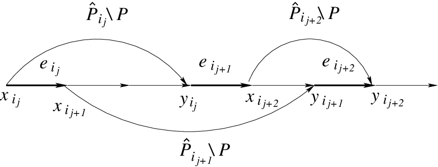
For $i=1,\ldots,k$ let $P_{i}$ be a $s$ – $t$ path associated with $e_{i}$ by a constraint of type (3) applied to $\mathbf{b}$ ; consequently $b(P\setminus P_{i})=c(P_{i}\setminus P)$ . We can assume without loss of generality that $P_{i}$ coincides with $P$ up to some vertex $x_{i}$ , then deviates from $P$ to avoid $e_{i}$ , and finally returns to $P$ at a vertex $y_{i}$ and coincides with $P$ from then on (clearly, it might happen that $s=x_{i}$ or $t=y_{i}$ ). Indeed, if $P_{i}$ deviates from $P$ more than once, one of these deviations is not necessary to avoid $e_{i}$ and can be replaced with the respective segment of $P$ without increasing the cost of $P_{i}$ . Among all paths of this form, let $\hat{P}_{i}$ be the one with the largest value of $y_{i}$ , i.e., the “rightmost” one. This path corresponds to an equality $I_{i}$ of the form $b_{x_{i}+1}+\dots+b_{y_{i}}=c(\hat{P}_{i}\setminus P)$ .

We construct a set $\mathcal{L}$ of equalities such that every variable $b_{i}$ appears in at least one of them. We construct $\mathcal{L}$ inductively as follows. Start by setting $\mathcal{L}=\{I_{1}\}$ . At the $j$ th step, suppose that all variables up to (but not including) $b_{i_{j}}$ appear in at least one equality in $\mathcal{L}$ . Add $I_{i_{j}}$ to $\mathcal{L}$ .

Note that for any $j$ we have $y_{i_{j+1}}>y_{i_{j}}$ . This is because the equalities added to $\mathcal{L}$ during the first $j$ steps did not cover $b_{i_{j+1}}$ . See Figure 3. Since $y_{i_{j+2}}>y_{i_{j+1}}$ , we must also have $x_{i_{j+2}}>y_{i_{j}}$ : otherwise, $\hat{P}_{i_{j+1}}$ would not be the “rightmost” constraint for $b_{i_{j+1}}$ . Therefore, the variables in $I_{i_{j+2}}$ and $I_{i_{j}}$ do not overlap, and hence no $b_{i}$ can appear in more than two equalities in $\mathcal{L}$ . Hence, adding up all of the equalities in $\mathcal{L}$ (and noting that the $b_{i}$ are non-negative) we obtain

2\sum_{i=1,\dots,k}b_{i}\geq\sum_{j~:~i_{j}\in\mathcal{L}}c(\hat{P_{j}}\setminus P).

On the other hand, each equality $I_{i}$ has a corresponding inequality based on constraint (2) applied to $\mathbf{b}^{\prime}$ , namely $b^{\prime}_{x_{i}+1}+\dots+b^{\prime}_{y_{i}}\leq c(\hat{P}_{i}\setminus P)$ . Summing these inequalities we have $\sum_{i=1,\dots,k}b^{\prime}_{i}\leq\sum_{j~:~i_{j}\in\mathcal{L}}c(\hat{P_{j}}\setminus P)$ . The result follows from this and the previous expression. ∎

Finally, we show that for matroids all four payment bounds coincide.

Theorem 15.

For any matroid $M=(\mathcal{E},\mathcal{F})$ with cost vector $\mathbf{c}$ , ${{\mathrm{TUmax}}({\mathbf{c}})}/{\mathrm{TUmin}}({\mathbf{c}})=1$ .

Proof.

Let $S$ , $|S|=k$ be the lexicographically-least cheapest base of $M$ . We can assume without loss of generality that $S=\{e_{1},\dots,e_{k}\}$ . Let $\mathbf{b}=(b_{1},\dots,b_{k})$ and $\mathbf{b}^{\prime}=(b^{\prime}_{1},\dots,b^{\prime}_{k})$ be bid vectors that correspond to ${\mathrm{TUmin}}({\mathbf{c}})$ and ${\mathrm{TUmax}}({\mathbf{c}})$ , respectively. For the bid vector $\mathbf{b}$ and any $e_{i}\in S$ , consider a constraint in (2) that is tight for $e_{i}$ and the base $S^{\prime}$ that is associated with this constraint. Suppose $S\setminus S^{\prime}=\{e_{i_{1}},\dots,e_{i_{t}}\}$ , i.e., the tight constraint for $e_{i}$ is of the form $b_{i_{1}}+\dots+b_{i_{t}}=c(S^{\prime}\setminus S)$ , $i\in\{i_{i_{1}},\dots,i_{i_{t}}\}$ . By Proposition 1 there is a mapping $f$ such that $S^{\prime}\setminus S=\{f(e_{i_{1}}),\dots,f(e_{i_{t}})\}$ and for $j=1,\dots,t$ the set $S\setminus\{e_{i_{j}}\}\cup\{f(e_{i_{j}})\}$ is a base. Therefore by condition (2) we have $b(e_{i_{j}})\leq c(f(e_{i_{j}}))$ for all $j=1,\dots,t$ . Consequently, it must be the case that all these constraints are tight as well, and in particular we have $b_{i}=c(f(e_{i}))$ . On the other hand, as $S\setminus\{e_{i}\}\cup\{f(e_{i})\}\in\mathcal{F}$ , we also have $b^{\prime}_{i}\leq c(f(e_{i}))=b_{i}$ . As this holds for any $i=1,\dots,k$ , we have ${\mathrm{TUmax}}({\mathbf{c}})\leq{\mathrm{TUmin}}({\mathbf{c}})$ . Since also ${\mathrm{TUmin}}({\mathbf{c}})\leq{\mathrm{TUmax}}({\mathbf{c}})$ , the theorem follows. ∎

5 Truthful mechanisms for vertex cover

Recall that for a vertex-cover auction on a graph $G=(V,E)$ , an allocation rule is an algorithm that takes as input a bid $b_{v}$ for each vertex $v$ and returns a vertex cover $\hat{S}$ of $G$ . As explained in Section 2, we can combine any monotone allocation rule with threshold payments to obtain a truthful auction.

Two natural examples of monotone allocation rules are $VCG$ , which finds an optimal vertex cover, and the mechanism $\mathcal{M}_{GR}$ that uses the greedy allocation algorithm. However, $VCG$ cannot be guaranteed to run in polynomial time unless $P=NP$ and $\mathcal{M}_{GR}$ has a worst-case approximation ratio of $\log n$ .

Another approximation algorithm for (weighted) vertex cover, which has approximation ratio 2, is the local ratio algorithm $A_{LR}$ [2, 3]. This algorithm considers the edges of $G$ one by one. Given an edge $e=(u,v)$ , it computes $\epsilon=\min\{b_{u},b_{v}\}$ and sets $b_{u}=b_{u}-\epsilon$ , $b_{v}=b_{v}-\epsilon$ . After all edges have been processed, $A_{LR}$ returns the set of vertices $\{v\mid b_{v}=0\}$ . It is not hard to check that if the order in which the edges are considered is independent of the bids, then this algorithm is monotone as well. Hence, we can use it to construct a truthful auction $\mathcal{M}_{LR}$ that is guaranteed to select a vertex cover whose cost is within a factor of 2 from the optimal.

However, while the quality of the solution produced by $A_{LR}$ is much better than that of $\mathcal{M}_{GR}$ , we still need to show that its total payment is not too high. In the next subsection, we bound the frugality ratio of $\mathcal{M}_{LR}$ (and, more generally, all algorithms that satisfy the condition of local optimality, defined later) by $2\Delta$ , where $\Delta$ is the maximum degree of $G$ . We then prove a matching lower bound showing that for some graphs the frugality ratio of any truthful auction is at least $\Delta/2$ .

5.1 Upper bound

For vertices $v$ and $w$ , $v\sim w$ means that there is an edge between $v$ and $w$ . We say that an allocation rule is locally optimal if whenever $b_{v}>\sum_{w\sim v}b_{w}$ , the vertex $v$ is not chosen. Note that for any such rule the threshold bid $t_{v}$ of $v$ satisfies $t_{v}\leq\sum_{w\sim v}b_{w}$ .

Remark 3.

The mechanisms $VCG$ , $\mathcal{M}_{GR}$ , and $\mathcal{M}_{LR}$ are locally optimal.

Theorem 16.

Any vertex cover auction $\mathcal{M}$ on a graph with maximum degree $\Delta$ that has a locally optimal and monotone allocation rule and pays each agent its threshold bid has frugality ratio $\phi_{\mathrm{NTUmin}}(\mathcal{M})\leq 2\Delta$ .

To prove Theorem 16, we first show that the total payment of any locally optimal mechanism does not exceed $\Delta c(V)$ . We then demonstrate that ${\mathrm{NTUmin}}({\mathbf{c}})\geq c(V)/2$ . By combining these two results, the theorem follows.

Lemma 17.

Let $G=(V,E)$ be a graph with maximum degree $\Delta$ . Let $\mathcal{M}$ be a vertex-cover auction on $G$ that satisfies the conditions of Theorem 16. Then for any cost vector $\mathbf{c}$ , the total payment of $\mathcal{M}$ satisfies $p_{\mathcal{M}}({\mathbf{c}})\leq\Delta c(V)$ .

Proof.

First note that any such auction is truthful, so we can assume that each agent’s bid is equal to its cost. Let $\hat{S}$ be the vertex cover selected by $\mathcal{M}$ . Then by local optimality

p_{\mathcal{M}}({\mathbf{c}})=\sum_{v\in\hat{S}}t_{v}\leq\sum_{v\in\hat{S}}\sum_{w\sim v}b_{w}=\sum_{v\in\hat{S}}\sum_{w\sim v}c_{w}\leq\sum_{w\in V}\Delta c_{w}=\Delta c(V).

∎

We now derive a lower bound on ${\mathrm{TUmax}}({\mathbf{c}})$ ; while not essential for the proof of Theorem 16, it helps us build the intuition necessary for that proof.

Lemma 18.

For a vertex cover instance $G=(V,E)$ in which $S$ is a minimum-cost vertex cover with respect to cost vector $\mathbf{c}$ , ${\mathrm{TUmax}}({\mathbf{c}},S)\geq c(V\setminus S)$ .

Proof.

For a vertex $w$ with at least one neighbour in $S$ , let $d(w)$ denote the number of neighbours that $w$ has in $S$ . Consider the bid vector $\mathbf{b}$ in which, for each $v\in S$ , $b_{v}=\sum_{w\sim v,w\not\in S}c_{w}/d(w)$ . Then $\sum_{v\in S}b_{v}=\sum_{v\in S}\sum_{w\sim v,w\not\in S}c_{w}/d(w)=\sum_{w\notin S}c_{w}=c(V\setminus S)$ . To finish we want to show that $\mathbf{b}$ is feasible in the sense that it satisfies (2). Consider a vertex cover $T$ , and extend the bid vector $\mathbf{b}$ by assigning $b_{v}=c_{v}$ for $v\notin S$ . Then

b(T)=c(T\setminus S)+b(S\cap T)\geq c(T\setminus S)+\sum_{v\in S\cap T}\sum_{w\in\overline{S}\cap\overline{T}:w\sim v}c_{w}/d(w),

and since all edges between $\overline{S}\cap\overline{T}$ and $S$ go to $S\cap T$ , the right-hand-side is equal to

c(T\setminus S)+\sum_{w\in\overline{S}\cap\overline{T}}c_{w}=c(T\setminus S)+c(\overline{S}\cap\overline{T})=c(V\setminus S)=b(S).

∎

Next, we prove a lower bound on ${\mathrm{NTUmax}}({\mathbf{c}},S)$ ; we will then use it to obtain a lower bound on ${\mathrm{NTUmin}}({\mathbf{c}})$ .

Lemma 19.

For a vertex cover instance $G=(V,E)$ in which $S$ is a minimum-cost vertex cover with respect to cost vector $\mathbf{c}$ , ${\mathrm{NTUmax}}({\mathbf{c}},S)\geq c(V\setminus S)$ .

Proof.

If $c(S)\geq c(V\setminus S)$ , by condition (1) we are done. Therefore, for the rest of the proof we assume that $c(S)<c(V\setminus S)$ . We show how to construct a bid vector $(b_{e})_{e\in S}$ that satisfies conditions (1) and (2) such that $b(S)\geq c(V\setminus S)$ ; clearly, this implies ${\mathrm{NTUmax}}({\mathbf{c}},S)\geq c(V\setminus S)$ .

Recall that a network flow problem is described by a directed graph $\Gamma=(V_{\Gamma},E_{\Gamma})$ , a source node $s\in V_{\Gamma}$ , a sink node $t\in V_{\Gamma}$ , and a vector of capacity constraints $a_{e}$ , $e\in E_{\Gamma}$ . Consider a network $(V_{\Gamma},E_{\Gamma})$ such that $V_{\Gamma}=V\cup\{s,t\}$ , $E_{\Gamma}=E_{1}\cup E_{2}\cup E_{3}$ , where $E_{1}=\{(s,v)\mid v\in S\}$ , $E_{2}=\{(v,w)\mid v\in S,w\in V\setminus S,(v,w)\in E\}$ , $E_{3}=\{(w,t)\mid w\in V\setminus S\}$ . Since $S$ is a vertex cover for $G$ , no edge of $E$ can have both of its endpoints in $V\setminus S$ , and by construction, $E_{2}$ contains no edges with both endpoints in $S$ . Therefore, the graph $(V,E_{2})$ is bipartite with parts $(S,V\setminus S)$ .

Set the capacity constraints for $e\in E_{\Gamma}$ as follows: $a_{(s,v)}=c_{v}$ , $a_{(w,t)}=c_{w}$ , $a_{(v,w)}=+\infty$ for all $v\in S$ , $w\in V\setminus S$ . Recall that a cut is a partition of the vertices in $V_{\Gamma}$ into two sets $C_{1}$ and $C_{2}$ so that $s\in C_{1}$ , $t\in C_{2}$ ; we denote such a cut by $C=(C_{1},C_{2})$ . Abusing notation, we write $e=(u,v)\in C$ if $u\in C_{1},v\in C_{2}$ or $u\in C_{2},v\in C_{1}$ , and say that such an edge $e=(u,v)$ crosses the cut $C$ . The capacity of a cut $C$ is computed as ${\rm cap}(C)=\sum_{(v,w)\in C}a_{(v,w)}$ . We have ${\rm cap}(s,V\cup\{t\})=c(S)$ , ${\rm cap}(\{s\}\cup V,t)=c(V\setminus S)$ .

Let $C_{\min}=(\{s\}\cup S^{\prime}\cup W^{\prime},\{t\}\cup S^{\prime\prime}\cup W^{\prime\prime})$ be a minimum cut in $\Gamma$ , where $S^{\prime},S^{\prime\prime}\subseteq S$ , $W^{\prime},W^{\prime\prime}\subseteq V\setminus S$ . See Figure 4. As ${\rm cap}(C_{\min})\leq{\rm cap}(s,V\cup\{t\})=c(S)<+\infty$ , and any edge in $E_{2}$ has infinite capacity, no edge $(u,v)\in E_{2}$ crosses $C_{\min}$ .

Consider the network $\Gamma^{\prime}=(V_{\Gamma^{\prime}},E_{\Gamma^{\prime}})$ , where $V_{\Gamma^{\prime}}=\{s\}\cup S^{\prime}\cup W^{\prime}\cup\{t\}$ , $E_{\Gamma^{\prime}}=\{(u,v)\in E_{\Gamma}\mid u,v\in V_{\Gamma^{\prime}}\}$ . Clearly, $C^{\prime}=(\{s\}\cup S^{\prime}\cup W^{\prime},\{t\})$ is a minimum cut in $\Gamma^{\prime}$ (otherwise, there would exist a smaller cut for $\Gamma$ ). As ${\rm cap}(C^{\prime})=c(W^{\prime})$ , we have $c(S^{\prime})\geq c(W^{\prime})$ .

Now, consider the network $\Gamma^{\prime\prime}=(V_{\Gamma^{\prime\prime}},E_{\Gamma^{\prime\prime}})$ , where $V_{\Gamma^{\prime\prime}}=\{s\}\cup S^{\prime\prime}\cup W^{\prime\prime}\cup\{t\}$ , $E_{\Gamma^{\prime\prime}}=\{(u,v)\in E_{\Gamma}\mid u,v\in V_{\Gamma^{\prime\prime}}\}$ . Similarly, $C^{\prime\prime}=(\{s\},S^{\prime\prime}\cup W^{\prime\prime}\cup\{t\})$ is a minimum cut in $\Gamma^{\prime\prime}$ , ${\rm cap}(C^{\prime\prime})=c(S^{\prime\prime})$ . As the size of a maximum flow from $s$ to $t$ is equal to the capacity of a minimum cut separating $s$ and $t$ , there exists a flow ${\cal F}=(f_{e})_{e\in E_{\Gamma^{\prime\prime}}}$ of size $c(S^{\prime\prime})$ . This flow has to saturate all edges between $s$ and $S^{\prime\prime}$ , i.e., $f_{(s,v)}=c_{v}$ for all $v\in S^{\prime\prime}$ . Now, increase the capacities of all edges between $s$ and $S^{\prime\prime}$ to $+\infty$ . In the modified network, the capacity of a minimum cut (and hence the size of a maximum flow) is $c(W^{\prime\prime})$ , and a maximum flow ${\cal F}^{\prime}=(f^{\prime}_{e})_{e\in E_{\Gamma^{\prime\prime}}}$ can be constructed by greedily augmenting ${\cal F}$ .

Set $b_{v}=c_{v}$ for all $v\in S^{\prime}$ , $b_{v}=f^{\prime}_{(s,v)}$ for all $v\in S^{\prime\prime}$ . As ${\cal F}^{\prime}$ is constructed by augmenting ${\cal F}$ , we have $b_{v}\geq c_{v}$ for all $v\in S$ , i.e., condition (1) is satisfied.

Now, let us check that no vertex cover $T\subseteq V$ can violate condition (2). Set $T_{1}=T\cap S^{\prime}$ , $T_{2}=T\cap S^{\prime\prime}$ , $T_{3}=T\cap W^{\prime}$ , $T_{4}=T\cap W^{\prime\prime}$ ; our goal is to show that $b(S^{\prime}\setminus T_{1})+b(S^{\prime\prime}\setminus T_{2})\leq c(T_{3})+c(T_{4})$ . Consider all edges $(u,v)\in E$ such that $u\in S^{\prime}\setminus T_{1}$ . If $(u,v)\in E_{2}$ then $v\in T_{3}$ (no edge in $E_{2}$ can cross the cut), and if $u,v\in S$ then $v\in T_{1}\cup T_{2}$ . Hence, $T_{1}\cup T_{3}\cup S^{\prime\prime}$ is a vertex cover for $G$ , and therefore $c(T_{1})+c(T_{3})+c(S^{\prime\prime})\geq c(S)=c(T_{1})+c(S^{\prime}\setminus T_{1})+c(S^{\prime\prime})$ . Consequently, $c(T_{3})\geq c(S^{\prime}\setminus T_{1})=b(S^{\prime}\setminus T_{1})$ . Now, consider the vertices in $S^{\prime\prime}\setminus T_{2}$ . Any edge in $E_{2}$ that starts in one of these vertices has to end in $T_{4}$ (this edge has to be covered by $T$ , and it cannot go across the cut). Therefore, the total flow out of $S^{\prime\prime}\setminus T_{2}$ is at most the total flow out of $T_{4}$ , i.e., $b(S^{\prime\prime}\setminus T_{2})\leq c(T_{4})$ . Hence, $b(S^{\prime}\setminus T_{1})+b(S^{\prime\prime}\setminus T_{2})\leq c(T_{3})+c(T_{4})$ . ∎

Finally, we derive a lower bound on the payment bound that is of interest to us, namely, ${\mathrm{NTUmin}}({\mathbf{c}})$ .

Lemma 20.

For a vertex cover instance $G=(V,E)$ in which $S$ is a minimum-cost vertex cover with respect to cost vector $\mathbf{c}$ , ${\mathrm{NTUmin}}({\mathbf{c}},S)\geq c(V\setminus S)$ .

Proof.

Suppose for contradiction that ${\mathbf{c}}$ is a cost vector with minimum-cost vertex cover $S$ and ${\mathrm{NTUmin}}({\mathbf{c}},S)<c(V\setminus S)$ . Let ${\mathbf{b}}$ be the corresponding bid vector and let ${\mathbf{c}}^{\prime}$ be a new cost vector with $c^{\prime}_{v}=b_{v}$ for $v\in S$ and $c^{\prime}_{v}=c_{v}$ for $v\not\in S$ . Condition (2) guarantees that $S$ is an optimal solution to the cost vector ${\mathbf{c}}^{\prime}$ . Now compute a bid vector ${\mathbf{b}}^{\prime}$ corresponding to ${\mathrm{NTUmax}}({\mathbf{c}}^{\prime},S)$ . We claim that $b^{\prime}_{v}=c^{\prime}_{v}$ for any $v\in S$ . Indeed, suppose that $b^{\prime}_{v}>c^{\prime}_{v}$ for some $v\in S$ ( $b^{\prime}_{v}=c^{\prime}_{v}$ for $v\not\in S$ by construction). As ${\mathbf{b}}$ satisfies conditions (1)–(3), among the inequalities in (2) there is one that is tight for $v$ and the bid vector ${\mathbf{b}}$ . That is, $b(S\setminus T)=c(T\setminus S)$ . By the construction of ${\mathbf{c}}^{\prime}$ , $c^{\prime}(S\setminus T)=c^{\prime}(T\setminus S)$ . Now since $b^{\prime}_{w}\geq c^{\prime}_{w}$ for all $w\in S$ , $b^{\prime}_{v}>c^{\prime}_{v}$ implies $b^{\prime}(S\setminus T)>c^{\prime}(S\setminus T)=c^{\prime}(T\setminus S)$ . But this violates (2). So we now know ${\mathbf{b}}^{\prime}={\mathbf{c}}^{\prime}$ . Hence, we have ${\mathrm{NTUmax}}({\mathbf{c}}^{\prime},S)=\sum_{v\in S}b_{v}={\mathrm{NTUmin}}({\mathbf{c}},S)<c(V\setminus S)$ , giving a contradiction to the fact that ${\mathrm{NTUmax}}({\mathbf{c}}^{\prime},S)\geq c^{\prime}(V\setminus S)$ which we proved in Lemma 19. ∎

As ${\mathrm{NTUmin}}({\mathbf{c}},S)$ satisfies condition (1), we have ${\mathrm{NTUmin}}({\mathbf{c}},S)\geq c(S)$ . Together will Lemma 20, this implies ${\mathrm{NTUmin}}({\mathbf{c}},S)\geq\max\{c(V\setminus S),c(S)\}\geq c(V)/2$ . Combined with Lemma 17, this completes the proof of Theorem 16.

Remark 4.

As ${\mathrm{NTUmin}}({\mathbf{c}})\leq{\mathrm{NTUmax}}({\mathbf{c}})\leq{\mathrm{TUmax}}({\mathbf{c}})$ , our bound of $2\Delta$ extends to the smaller frugality ratios that we consider, i.e., $\phi_{\mathrm{NTUmax}}(\mathcal{M})$ and $\phi_{\mathrm{TUmax}}(\mathcal{M})$ . It is not clear whether it extends to the larger frugality ratio $\phi_{\mathrm{TUmin}}(\mathcal{M})$ . However, the frugality ratio $\phi_{\mathrm{TUmin}}(\mathcal{M})$ is not realistic because the payment bound ${\mathrm{TUmin}}({\mathbf{c}})$ is inappropriately low—we show in Section 6 that ${\mathrm{TUmin}}({\mathbf{c}})$ can be significantly smaller than the total cost of a cheapest vertex cover.

Extensions

We can also apply our results to monotone vertex-cover algorithms that do not necessarily output locally-optimal solutions. To do so, we simply take the vertex cover produced by any such algorithm and transform it into a locally-optimal one, considering the vertices in lexicographic order and replacing a vertex $v$ with its neighbours whenever $b_{v}>\sum_{u\sim v}b_{u}$ . Note that if a vertex $u$ gets added to the vertex cover during this process, it means that it has a neighbour whose bid is higher than $u$ ’s bid $b_{u}$ , so after one pass all vertices in the vertex cover satisfy $b_{v}\leq\sum_{u\sim v}b_{u}$ . This procedure is monotone in bids, and it can only decrease the cost of the vertex cover. Therefore, using it on top of a monotone allocation rule with approximation ratio $\alpha$ , we obtain a monotone locally-optimal allocation rule with approximation ratio $\alpha$ . Combining it with threshold payments, we get an auction with $\phi_{\mathrm{NTUmin}}\leq 2\Delta$ . Since any truthful auction has a monotone allocation rule, this procedure transforms any truthful mechanism for the vertex-cover problem into a frugal one while preserving the approximation ratio.

5.2 Lower bound

In this subsection, we prove that the upper bound of Theorem 16 is essentially optimal. Our proof uses the techniques of [9], where the authors prove a similar result for shortest-path auctions.

Theorem 21.

For any $\Delta>0$ , there exists a graph $G$ with $2\Delta$ vertices and degree $\Delta$ , such that for any truthful mechanism $\mathcal{M}$ on $G$ we have $\phi_{\mathrm{NTUmin}}(\mathcal{M})\geq\Delta/2$ .

Proof.

Let $G$ be a complete bipartite graph with parts $L$ and $R$ , $|L|=|R|=\Delta$ , thus $G$ has degree $\Delta$ .

We consider two families of cost vectors for $G$ . Under a cost vector ${\mathbf{x}}\in X$ , $G$ has one vertex of cost 1; all other vertices cost 0. Under a cost vector ${\mathbf{y}}\in Y$ , each of $L$ and $R$ has one vertex of cost 1, and all other vertices have cost 0. Clearly, $|X|=2\Delta$ , $|Y|=\Delta^{2}$ . We construct a bipartite graph $W$ with the vertex set $X\cup Y$ as follows.

Consider a cost vector ${\mathbf{y}}\in Y$ ; let its cost-1 vertices be $v_{l}\in L$ and $v_{r}\in R$ . By changing the cost of either of these vertices to 0, we obtain a cost vector in $X$ . Let ${\mathbf{x}}_{l}$ and ${\mathbf{x}}_{r}$ be the cost vectors obtained by changing the cost of $v_{l}$ and $v_{r}$ , respectively. The vertex cover chosen by $\mathcal{M}({\mathbf{y}})$ must either contain all vertices in $L$ or all vertices in $R$ . In the former case, we add to $W$ an edge from ${\mathbf{y}}$ to ${\mathbf{x}}_{l}$ and in the latter case we add to $W$ an edge from ${\mathbf{y}}$ to ${\mathbf{x}}_{r}$ (if the vertex cover includes all of $G$ , $W$ contains both of these edges).

The graph $W$ has at least $\Delta^{2}$ edges, so there must exist an ${\mathbf{x}}\in X$ of degree at least $\Delta/2$ . Let $\mathbf{y}_{1},\dots,\mathbf{y}_{\Delta/2}$ be the other endpoints of the edges incident to ${\mathbf{x}}$ , and for each $i=1,\dots,\Delta/2$ , let $v_{i}$ be the vertex of $G$ whose cost is different under ${\mathbf{x}}$ and ${\mathbf{y}}_{i}$ ; note that all $v_{i}$ are distinct.

It is not hard to see that ${\mathrm{NTUmin}}({\mathbf{x}})\leq 1$ : the cheapest vertex cover contains the all-0 part of $G$ , and we can satisfy conditions (1)–(3) by allowing one of the vertices in the all-0 part of each block to bid 1, while all other vertices in the cheapest set bid 0.

On the other hand, by monotonicity of $\mathcal{M}$ we have $v_{i}\in\mathcal{M}({\mathbf{x}})$ for $i=1,\dots,\Delta/2$ ( $v_{i}$ is in the winning set under ${\mathbf{y}}_{i}$ , and ${\mathbf{x}}$ is obtained from ${\mathbf{y}}_{i}$ by decreasing the cost of $v_{i}$ ), and moreover, the threshold bid of each $v_{i}$ is at least 1, so the total payment of $\mathcal{M}$ on ${\mathbf{x}}$ is at least $\Delta/2$ . Hence, $\phi_{\mathrm{NTUmin}}(\mathcal{M})\geq\mathcal{M}({\mathbf{x}})/{\mathrm{NTUmin}}({\mathbf{x}})\geq\Delta/2$ . ∎

Remark 5.

Theorem 21 can be extended to apply to graphs with degree $\Delta$ of unlimited size: a similar argument applies to any graph made up of multiple copies of the bipartite graph $G$ in the proof. The resulting lower bound is still $\Delta/2$ , i.e., it does not depend on the size of the graph.

Remark 6.

The lower bound of Theorem 21 can be generalised to randomised mechanisms, where a randomised mechanism is considered to be truthful if it can be represented as a probability distribution over truthful mechanisms. In this case, instead of choosing the vertex ${\mathbf{x}}\in X$ with the highest degree, we put both $({\mathbf{y}},{\mathbf{x}}_{l})$ and $({\mathbf{y}},{\mathbf{x}}_{r})$ into $W$ , label each edge with the probability that the respective part of the block is chosen, and pick ${\mathbf{x}}\in X$ with the highest weighted degree.

6 Properties of the payment bounds

In this section we consider several desirable properties of payment bounds and evaluate the four payment bounds proposed in this paper with respect to them. The particular properties that we are interested in are the relationship with other reasonable bounds, such as the total cost of the cheapest set $S$ (Section 6.1), or the total VCG payment (Section 6.2). We also consider independence of the choice of $S$ (Section 6.3), monotonicity (Section 6.4.1), computational tractability (Section 6.4.2).

6.1 Comparison with total cost of winning set

The basic property of individual rationality dictates that the total payment must be at least the total cost of the selected winning set. In this section we show that amongst the payment bounds we consider here, ${\mathrm{TUmin}}({\mathbf{c}})$ may be less than the cost of the winning set $S$ . For such set systems, ${\mathrm{TUmin}}({\mathbf{c}})$ may as a result be too low to be realistic.

Clearly, ${\mathrm{NTUmax}}({\mathbf{c}})$ and ${\mathrm{NTUmin}}({\mathbf{c}})$ are at least the cost of $S$ due to condition (1), and so is ${\mathrm{TUmax}}({\mathbf{c}})$ , since ${\mathrm{TUmax}}({\mathbf{c}})\geq{\mathrm{NTUmax}}({\mathbf{c}})$ . However, ${\mathrm{TUmin}}({\mathbf{c}})$ fails this test. The example of Proposition 4 (part $(iii)$ ) shows that for path auctions, ${\mathrm{TUmin}}({\mathbf{c}})$ can be smaller than the total cost by a factor of 2. Moreover, there are set systems and cost vectors for which ${\mathrm{TUmin}}({\mathbf{c}})$ is smaller than the cost of the cheapest set $S$ by a factor of $\Omega(n)$ . Consider, for example, the vertex-cover auction for the graph of Proposition 10 with the costs $c_{X_{1}}=\dots=c_{X_{n-2}}=c_{X_{n-1}}=1$ , $c_{X_{0}}=0$ . The cost of a cheapest vertex cover is $n-2$ , and the lexicographically first vertex cover of cost $n-2$ is $\{X_{0},X_{1},\dots,X_{n-2}\}$ . The constraints in (2) are $b_{X_{i}}+b_{X_{0}}\leq c_{X_{n-1}}=1$ . Clearly, we can satisfy conditions (2) and (3) by setting $b_{X_{1}}=\dots=b_{X_{n-2}}=0$ , $b_{X_{0}}=1$ , which means that ${\mathrm{TUmin}}({\mathbf{c}})\leq 1$ . This example suggests that the payment bound ${\mathrm{TUmin}}({\mathbf{c}})$ is sometimes too strong to be realistic, since it can be substantially lower than the cost of a cheapest feasible set.

Note, however, that this is not an issue for matroid auctions becuase, for matroids, all four payment bounds have the same value. The paper [16] shows that if the feasible sets are the bases of a monopoly-free matroid, then $\phi_{\mathrm{NTUmin}}(\mathrm{VCG})=1$ . It is not difficult to see that this is also the case for other payment bounds.

Claim 22.

For any monopoly-free matroid, we have

\phi_{\mathrm{TUmin}}(\mathrm{VCG})=\phi_{\mathrm{TUmax}}(\mathrm{VCG})=\phi_{\mathrm{NTUmax}}(\mathrm{VCG})=\phi_{\mathrm{NTUmin}}(\mathrm{VCG})=1.

Proof.

The claim follows immediately from Theorem 15. Alternatively, it is not hard to check that the argument used in [16] for ${\mathrm{NTUmin}}({\mathbf{c}})$ does not use condition (1) at all and hence it works for ${\mathrm{TUmin}}({\mathbf{c}})$ as well. ∎

6.2 Comparison with VCG payments

Another measure of suitability for payment bounds is that they should not result in frugality ratios that are less then 1 for well-known truthful mechanisms¹¹ 1 It is too much to ask that they do not result in frugality ratios that are less than 1 for all mechanisms, since this can typically be subverted by artificial mechanisms.. If this is indeed the case, the payment bound may be too weak, as it becomes too easy to design mechanisms that perform well with respect to it. It particular, a reasonable requirement is that a payment bound should not exceed the total payment of the classical VCG mechanism.

The following proposition shows that ${\mathrm{NTUmax}}({\mathbf{c}})$ , and therefore also ${\mathrm{NTUmin}}({\mathbf{c}})$ and ${\mathrm{TUmin}}({\mathbf{c}})$ , do not exceed the VCG payment $p_{\mathrm{VCG}}({\mathbf{c}})$ . The proof essentially follows the argument of Proposition 7 of [16].

Proposition 23.

For any set-system auction, $\phi_{\mathrm{NTUmax}}(\mathrm{VCG})\geq 1$ .

Proof.

Let $S$ be a winning set chosen by VCG (hence, a cheapest set). Suppose $e\in S$ . The VCG payment $p_{e}$ is $\min_{T:e\notin T}\{c_{e}+c(T)-c(S)\}$ . Let $T_{e}$ be a feasible set $T$ which achieves the minimum, so $p_{e}=c(T_{e})-c(S\setminus\{e\})$ . But constraint (2) gives $b(S\setminus T)\leq c(T\setminus S)$ for all $T$ , so since $e\notin T_{e}$ , $b_{e}+b((S\setminus T_{e})\setminus\{e\})\leq c(T_{e}\setminus S)$ , so

b_{e}\leq c(T_{e}\setminus S)-b((S\setminus T_{e})\setminus\{e\}).

(

4

)

Now by constraint (1), $b((S\setminus T_{e})\setminus\{e\})\geq c((S\setminus T_{e})\setminus\{e\})$ , so (4) gives

$b_{e}$	$\leq c(T_{e}\setminus S)-c((S\setminus T_{e})\setminus\{e\})$
	$=c(T_{e}\setminus S)+c(T_{e}\cap S)-c((S\setminus T_{e})\setminus\{e\})-c(T_{e}\cap S)$
	$\leq c(T_{e})-c(S\setminus\{e\})$
	$=p_{e}.$

Thus, every winner’s payment is at least his bid, so the result follows. ∎

Proposition 23 shows that none of the payment bounds ${\mathrm{TUmin}}({\mathbf{c}})$ , ${\mathrm{NTUmin}}({\mathbf{c}})$ and ${\mathrm{NTUmax}}({\mathbf{c}})$ exceeds the payment of VCG. However, the payment bound ${\mathrm{TUmax}}({\mathbf{c}})$ can be larger that the total VCG payment. In particular, for the instance in Proposition 10, the VCG payment is smaller than ${\mathrm{TUmax}}({\mathbf{c}})$ by a factor of $n-2$ . We have already seen that ${\mathrm{TUmax}}({\mathbf{c}})\geq n-2$ . On the other hand, under VCG, the threshold bid of any $X_{i}$ , $i=1,\dots,n-2$ , is 0: if any such vertex bids above 0, it is deleted from the winning set together with $X_{0}$ and replaced with $X_{n-1}$ . Similarly, the threshold bid of $X_{0}$ is 1, because if $X_{0}$ bids above 1, it can be replaced with $X_{n-1}$ . So the VCG payment is $1$ .

This result is not surprising: the definition of ${\mathrm{TUmax}}({\mathbf{c}})$ implicitly assumes there is co-operation between the agents, while the computation of VCG payments does not take into account any interaction between them. Indeed, co-operation enables the agents to extract higher payments under VCG. That is, VCG is not group-strategyproof. This suggests that as a payment bound, ${\mathrm{TUmax}}({\mathbf{c}})$ may be too liberal, at least in a context where there is little or no co-operation between agents. Perhaps ${\mathrm{TUmax}}({\mathbf{c}})$ can be a good benchmark for measuring the performance of mechanisms designed for agents that can form coalitions or make side payments to each other, in particular, group-strategyproof mechanisms.

Another setting in which bounding $\phi_{\mathrm{TUmax}}$ is still of some interest is when, for the underlying problem, the optimal allocation and VCG payments are NP-hard to compute. In this case, finding a polynomial-time computable mechanism with good frugality ratio with respect to ${\mathrm{TUmax}}({\mathbf{c}})$ is a non-trivial task, while bounding the frugality ratio with respect to more challenging payment bounds could be too difficult. To illustrate this point, compare the proofs of Lemma 18 and Lemma 19: both require some effort, but the latter is much more difficult than the former.

6.3 The choice of $S$

All payment bounds defined in this paper correspond to the total bid of all elements in a cheapest feasible set, where ties are broken lexicographically. While this definition ensures that our payment bounds are well-defined, the particular choice of the draw-resolution rule appears arbitrary, and one might ask whether our payment bounds are sufficiently robust to be independent of this choice. It turns out that is indeed the case for ${\mathrm{NTUmin}}({\mathbf{c}})$ and ${\mathrm{NTUmax}}({\mathbf{c}})$ .

Proposition 24.

The values of $NTUMinS$ and ${\mathrm{NTUmax}}({\mathbf{c}},S)$ do not depend on the choice of $S$ .

Proof.

Consider two feasible sets $S_{1}$ and $S_{2}$ that have the same cost. In the computation of ${{\mathrm{NTUmin}}({\mathbf{c}},S_{1})}$ , all vertices in $S_{1}\setminus S_{2}$ would have to bid their true cost, since otherwise $S_{2}$ would become cheaper than $S_{1}$ . Hence, any bid vector for $S_{1}$ can only have $b_{e}\neq c_{e}$ for $e\in S_{1}\cap S_{2}$ , and hence constitutes a valid bid vector for $S_{2}$ (in the context of ${{\mathrm{NTUmin}}({\mathbf{c}},S_{2})}$ ) and vice versa. A similar argument applies to ${\mathrm{NTUmax}}({\mathbf{c}})$ . ∎

However, for ${\mathrm{TUmin}}({\mathbf{c}})$ and ${\mathrm{TUmax}}({\mathbf{c}})$ this is not the case. For example, consider the set system

\mathcal{E}=\{e_{1},e_{2},e_{3},e_{4},e_{5}\},\mathcal{F}=\left\{S_{1}=\{e_{1},e_{2}\},S_{2}=\{e_{2},e_{3},e_{4}\},S_{3}=\{e_{4},e_{5}\}\right\}

with the costs $c_{1}=2$ , $c_{2}=c_{3}=c_{4}=1$ , $c_{5}=3$ . The cheapest sets are $S_{1}$ and $S_{2}$ . Now ${{\mathrm{TUmax}}({\mathbf{c}},S_{1})}\leq 4$ , as the total bid of the elements in $S_{1}$ cannot exceed the total cost of $S_{3}$ . On the other hand, ${{\mathrm{TUmax}}({\mathbf{c}},S_{2})}\geq 5$ , as we can set $b_{2}=3,b_{3}=0,b_{4}=2$ . Similarly, ${{\mathrm{TUmin}}({\mathbf{c}},S_{1})}=4$ , because the equalities in (3) are $b_{1}=2$ and $b_{1}+b_{2}=4$ . But ${{\mathrm{TUmin}}({\mathbf{c}},S_{2})}\leq 3$ , since we can set $b_{2}=1$ , $b_{3}=2$ , $b_{4}=0$ .

6.4 Negative results for ${\mathrm{NTUmin}}({\mathbf{c}})$ and ${\mathrm{TUmin}}({\mathbf{c}})$

The results in [16] and our vertex cover results are proved for the frugality ratio $\phi_{\mathrm{NTUmin}}$ . Indeed, it can be argued that $\phi_{\mathrm{NTUmin}}$ is the “best” definition of frugality ratio, because among those payment bounds that are at least as large as the cost of a cheapest feasible set, it is most demanding of the algorithm. However, ${\mathrm{NTUmin}}({\mathbf{c}})$ is not always the easiest or the most natural payment bound to work with. In this subsection, we discuss several disadvantages of ${\mathrm{NTUmin}}({\mathbf{c}})$ (and also ${\mathrm{TUmin}}({\mathbf{c}})$ ) as compared with ${\mathrm{NTUmax}}({\mathbf{c}})$ and ${\mathrm{TUmax}}({\mathbf{c}})$ .

6.4.1 Nonmonotonicity

²² 2 Simultaneously and independently of our work, Chen and Karlin [6] studied the issue of nonmonotonicity of

{\mathrm{NTUmin}}({\mathbf{c}})

in much more detail. While some of our results on

{\mathrm{NTUmin}}({\mathbf{c}})

are subsumed by their work, we present our results here as we feel that they are relevant in the context of this paper, and furthermore, they also apply to

{\mathrm{TUmin}}({\mathbf{c}})

The first problem with ${\mathrm{NTUmin}}({\mathbf{c}})$ is that it is not monotone with respect to $\mathcal{F}$ , in that it may increase when one adds a feasible set to $\mathcal{F}$ . (It is, however, monotone in the sense that a losing agent cannot become a winner by raising its cost.) Intuitively, a good payment bound should satisfy this monotonicity requirement, as adding a feasible set increases the competition, so it should drive the prices down. Note that this is indeed the case for ${\mathrm{NTUmax}}({\mathbf{c}})$ and ${\mathrm{TUmax}}({\mathbf{c}})$ since a new feasible set adds a constraint in (2), thus limiting the solution space for the respective linear program (recall Remark 1).

Proposition 25.

Adding a feasible set to $\mathcal{F}$ can increase ${\mathrm{NTUmin}}({\mathbf{c}})$ and ${\mathrm{TUmin}}({\mathbf{c}})$ by a factor of $\Omega(n)$ , where $n$ is the number of agents.

Proof.

Let $\mathcal{E}=\{x,x^{\prime},y_{1},\ldots,y_{n},z_{1},\ldots,z_{n}\}$ . Let $Y=\{y_{1},\ldots,y_{n}\}$ , $S=Y\cup\{x\}$ , $T_{i}=Y\setminus\{y_{i}\}\cup\{z_{i}\}$ , $i=1,\dots,n$ , and suppose that $\mathcal{F}=\{S,T_{1},\ldots,T_{n}\}$ . The costs are $c_{x}=0$ , $c_{x^{\prime}}=0$ , $c_{y_{i}}=0$ , $c_{z_{i}}=1$ for $i=1,\dots,n$ . Note that $S$ is a cheapest feasible set. For $\mathcal{F}$ , the bid vector $b_{y_{1}}=\dots=b_{y_{n}}=0$ , $b_{x}=1$ satisfies (1), (2), and (3), so ${\mathrm{TUmin}}({\mathbf{c}})\leq{\mathrm{NTUmin}}({\mathbf{c}})\leq 1$ .

Let $S^{\prime}=Y\cup\{x^{\prime}\}$ . For $\mathcal{F}\cup\{S^{\prime}\}$ , $S$ is still the lexicographically-least cheapest set. Any optimal solution has $b_{x}=0$ (by constraint in (2) with $S^{\prime}$ ). Condition (3) for $y_{i}$ implies $b_{x}+b_{y_{i}}=c_{z_{i}}=1$ , so $b_{y_{i}}=1$ and ${\mathrm{NTUmin}}({\mathbf{c}})=n$ . As all constraints in (1) are of the form $b_{e}\geq 0$ , we also have ${\mathrm{TUmin}}({\mathbf{c}})=n$ . ∎

For path auctions, it has been shown [6] that ${\mathrm{NTUmin}}({\mathbf{c}})$ is non-monotone in a slightly different sense, i.e., with respect to adding a new edge (agent) rather than a new feasible set (a team of existing agents). We present that example here for completeness.

Proposition 26.

For shortest path auctions, adding an edge to the graph can increase ${\mathrm{NTUmin}}({\mathbf{c}})$ by a factor of $2$ .

Proof.

Consider the graph of Figure 1 with the edge costs $c_{AB}=c_{BC}=c_{CD}=0$ , $c_{AC}=c_{BD}=1$ . In this graph, $ABCD$ is the cheapest path, and it is easy to see that ${\mathrm{NTUmin}}({\mathbf{c}})=1$ with the bid vector $b_{AB}=b_{CD}=0$ , $b_{BC}=1$ . Now suppose that we add a new edge $\widehat{BC}$ of cost 0 between $B$ and $C$ , obtaining the graph of Figure 5. We can assume that the original shortest path $ABCD$ is the lexicographically first shortest path in the new graph, so it gets selected. However, now we have a new constraint in (2), namely, $b_{BC}\leq c_{\widehat{BC}}=0$ , so we have ${\mathrm{NTUmin}}({\mathbf{c}})=2$ with the bid vector $b_{AB}=b_{CD}=1$ , $b_{BC}=0$ . ∎

Remark 7.

It is not hard to modify the example of Proposition 26 so that the underlying graph has no multiple edges. Also, as all constraints in (1) are of the form $b_{e}\geq 0$ , it also applies to ${\mathrm{TUmin}}({\mathbf{c}})$ .

Remark 8.

We can also show that ${\mathrm{NTUmin}}({\mathbf{c}})$ and ${\mathrm{TUmin}}({\mathbf{c}})$ are non-monotone for vertex cover. In this case, adding a new feasible set corresponds to deleting edges from the graph. It turns out that deleting a single edge can increase ${\mathrm{NTUmin}}({\mathbf{c}})$ and ${\mathrm{TUmin}}({\mathbf{c}})$ by a factor of $n-2$ ; the construction is based on the graph and the cost vector used in Proposition 10.

6.4.2 NP-Hardness

Another problem with ${\mathrm{NTUmin}}({\mathbf{c}},S)$ is that it is NP-hard to compute, even if the number of feasible sets is polynomial in $n$ . Again, this puts it at a disadvantage compared to ${\mathrm{NTUmax}}({\mathbf{c}},S)$ and ${\mathrm{TUmax}}({\mathbf{c}},S)$ (see Remark 1).

Theorem 27.

Computing ${\mathrm{NTUmin}}({\mathbf{c}})$ is NP-hard, even when the lexicographically-least cheapest feasible set $S$ is given in the input.

Proof.

We reduce Exact cover by 3-sets(X3C) to our problem. An instance of X3C is given by a universe $G=\{g_{1},\dots,g_{n}\}$ and a collection of subsets $C_{1},\dots,C_{m}$ , $C_{i}\subset G$ , $|C_{i}|=3$ , where the goal is to decide whether one can cover $G$ by $n/3$ of these sets. Observe that if this is indeed the case, then each element of $G$ is contained in exactly one set of the cover.

Lemma 28.

Consider a minimisation problem ${\cal P}$ of the following form:
Minimise $\sum_{i=1,\dots,n}b_{i}$ under conditions

(1)

$b_{i}\geq 0$ for all $i=1,\dots,n$
(2)

$\sum_{i\in S_{j}}b_{i}\leq a_{j}$ for $j=1,\ldots,k$ ; subsets $S_{j}\subseteq\{1,\dots,n\}$
(3)

for each $b_{j}$ , one of the constraints in (2) involving it is tight.

For any such ${\cal P}$ , one can construct in polynomial time a set system and a vector of costs $\mathbf{c}$ such that ${\mathrm{NTUmin}}({\mathbf{c}})$ is the optimal solution to ${\cal P}$ .

Proof.

The construction is straightforward: there is an element $e_{i}$ of cost 0 for each $b_{i}$ , an element $e^{\prime}_{j}$ of cost $a_{j}$ for each $a_{j}$ , the feasible solutions are $\{e_{1},\dots,e_{n}\}$ , or any set obtained from $\{e_{1},\dots,e_{n}\}$ by replacing the elements indexed by $S_{j}$ , with $e^{\prime}_{j}$ . ∎

By this lemma, all we have to do to prove Theorem 27 is to show how to solve X3C by using the solution to a minimisation problem of the form given in Lemma 28. We do this as follows. For each $C_{i}$ , we introduce 4 variables $x_{i}$ , $\bar{x}_{i}$ , $a_{i}$ , and $b_{i}$ . Also, for each element $g_{j}$ of $G$ there is a variable $d_{j}$ . We use the following set of constraints:

•

In (1), we have constraints $x_{i}\geq 0$ , $\bar{x}_{i}\geq 0$ , $a_{i}\geq 0$ , $b_{i}\geq 0$ , $d_{j}\geq 0$ for all $i=1,\dots,m$ , $j=1,\dots,n$ .
•

In (2), for all $i=1,\dots,m$ , we have the following 5 constraints:
$x_{i}+\bar{x}_{i}\leq 1$
$x_{i}+a_{i}\leq 1$
$\bar{x}_{i}+a_{i}\leq 1$
$x_{i}+b_{i}\leq 1$
$\bar{x}_{i}+b_{i}\leq 1$ .

Also, for all $j=1,\dots,n$ we have the constraint $d_{j}+\sum_{i~:~g_{j}\in C_{i}}x_{i}\leq 1$ .

The goal is to minimize $Z=\sum_{i}(x_{i}+\bar{x}_{i}+a_{i}+b_{i})+\sum_{j}d_{j}$ .

Observe that for each $j$ , there is only one constraint involving $d_{j}$ , so by condition (3) it must be tight.

Consider the two constraints involving $a_{i}$ . One of them must be tight; either $x_{i}+a_{i}=1$ or $\bar{x}_{i}+a_{i}=1$ . It follows that $x_{1}+\bar{x}_{i}+a_{i}+b_{i}\geq 1$ . Hence, for any feasible solution to (1)–(3) we have $Z\geq m$ . Now, suppose that there is an exact set cover. Set $d_{j}=0$ for $j=1,\dots,n$ . Also, if $C_{i}$ is included in this cover, set $x_{i}=1$ , $\bar{x}_{i}=a_{i}=b_{i}=0$ , otherwise set $\bar{x}_{i}=1$ , $x_{i}=a_{i}=b_{i}=0$ . Clearly, all inequalities in (2) are satisfied (we use the fact that each element is covered exactly once), and for each variable, one of the constraints involving it is tight. This assignment results in $Z=m$ .

Conversely, suppose there is a feasible solution with $Z=m$ . As each addend of the form $x_{i}+\bar{x}_{i}+a_{i}+b_{i}$ contributes at least 1, we have $x_{i}+\bar{x}_{i}+a_{i}+b_{i}=1$ for all $i$ , $d_{j}=0$ for all $j$ . We will now show that for each $i$ , either $x_{i}=1$ and $\bar{x}_{i}=0$ , or $x_{i}=0$ and $\bar{x}_{i}=1$ . For the sake of contradiction, suppose that $x_{i}=\delta<1$ , $\bar{x}_{i}=\delta^{\prime}<1$ . As one of the constraints involving $a_{i}$ must be tight, we have $a_{i}\geq\min\{1-\delta,1-\delta^{\prime}\}$ . Similarly, $b_{i}\geq\min\{1-\delta,1-\delta^{\prime}\}$ . Hence, $x_{i}+\bar{x}_{i}+a_{i}+b_{i}\geq\delta+\delta^{\prime}+2\min\{1-\delta,1-\delta^{\prime}\}>1$ . This contradicts the previously noted equality $x_{i}+\bar{x}_{i}+a_{i}+b_{i}=1$ .

To finish the proof, note that for each $j=1,\dots,n$ we have $x_{i_{1}}+\dots+x_{i_{k}}+d_{j}=1$ and $d_{j}=0$ , so the subsets that correspond to $x_{i}=1$ constitute a set cover. ∎

Remark 9.

In the proofs of Theorem 27 all constraints in (1) are of the form $b_{e}\geq 0$ . Hence, the same result is true for ${\mathrm{TUmin}}({\mathbf{c}})$ .

Remark 10.

For shortest-path auctions, the size of $\mathcal{F}$ can be superpolynomial. However, there is a polynomial-time separation oracle for constraints in (2) (to construct one, use any algorithm for finding shortest paths), so one can compute ${\mathrm{NTUmax}}({\mathbf{c}})$ and ${\mathrm{TUmax}}({\mathbf{c}})$ in polynomial time. On the other hand, recently and independently it was shown [6] that computing ${\mathrm{NTUmin}}({\mathbf{c}})$ for shortest-path auctions is NP-hard.

Acknowledgements. We thanks David Kempe for suggesting the “diamond graph” auction and the cost vector used in the proof of Proposition 4[(i)].

References

[1] A. Archer and E. Tardos, Frugal path mechanisms. In Proceedings of the 13th Annual ACM-SIAM Symposium on Discrete Algorithms, pages 991–999, 2002.
[2] R. Bar-Yehuda, K. Bendel, A. Freund, and D. Rawitz, Local ratio: A unified framework for approximation algorithms. In Memoriam: Shimon Even 1935-2004. ACM Comput. Surv., 36(4):422–463, 2004.
[3] R. Bar-Yehuda and S. Even, A local-ratio theorem for approximating the weighted vertex cover problem. Annals of Discrete Mathematics, 25:27–46, 1985.
[4] E. Clarke, Multipart pricing of public goods. Public Choice, 8:17–33, 1971.
[5] G. Calinescu, Bounding the payment of approximate truthful mechanisms. In Proceedings of the 15th International Symposium on Algorithms and Computation, pages 221–233, Dec. 2004.
[6] N. Chen and A.R. Karlin, Cheap labor can be expensive, In Proceedings of the 18th Annual ACM-SIAM Symposium on Discrete Algorithms, pages 707–715, Jan. 2007.
[7] A. Czumaj and A. Ronen, On the expected payment of mechanisms for task allocation. In Proceedings of the 5th ACM Conference on Electronic Commerce (EC’04), 2004.
[8] E. Elkind, True costs of cheap labor are hard to measure: edge deletion and VCG payments in graphs. In Proceedings of the 6th ACM Conference on Electronic Commerce (EC’05), 2005.
[9] E. Elkind, A. Sahai, and K. Steiglitz, Frugality in path auctions. In Proceedings of the 15th Annual ACM-SIAM Symposium on Discrete Algorithms, pages 694–702, 2004.
[10] J. Feigenbaum, C. H. Papadimitriou, R. Sami, and S. Shenker, A BGP-based mechanism for lowest-cost routing. In Proceedings of the 21st Symposium on Principles of Distributed Computing, pages 173–182, 2002.
[11] A. Fiat, A. Goldberg, J. Hartline, and A. Karlin, Competitive generalized auctions. In Proceedings of the 34th Annual ACM Symposium on Theory of Computation, pages 72–81, 2002.
[12] R. Garg, V. Kumar, A. Rudra and A. Verma, Coalitional games on graphs: core structures, substitutes and frugality. In Proceedings of the 4th ACM Conference on Electronic Commerce (EC’03), 2005.
[13] A. Goldberg, J. Hartline, and A. Wright, Competitive auctions and digital goods. In Proceedings of the 12th Annual ACM-SIAM Symposium on Discrete Algorithms, pages 735–744, 2001.
[14] T. Groves, Incentives in teams. Econometrica, 41(4):617–631, 1973.
[15] N. Immorlica, D. Karger, E. Nikolova, and R. Sami, First-price path auctions. In Proceedings of the 6th ACM Conference on Electronic Commerce (EC’05), 2005.
[16] A. R. Karlin, D. Kempe, and T. Tamir Beyond VCG: Frugality of Truthful Mechanisms. In Proceedings of the 46th Annual IEEE Symposium on Foundations of Computer Science, pages 615–624, Oct. 2005.
[17] N. Nisan and A. Ronen, Algorithmic mechanism design. In Proceedings of the 31st Annual ACM Symposium on Theory of Computation, pages 129–140, 1999.
[18] N. Nisan and A. Ronen, Computationally feasible VCG mechanisms. In Proceedings of the 2nd ACM Conference on Electronic Commerce (EC’00), pages 242–252, 2000.
[19] J. Oxley, Matroid theory. The Clarendon Press Oxford University Press, New York, 1992.
[20] A. Ronen and R. Talisman, Towards generic low payment mechanisms for decentralized task allocation. In Proceedings of the 7th International IEEE Conference on E-Commerce Technology, 2005.
[21] K. Talwar, The price of truth: frugality in truthful mechanisms. In Proceedings of 20th International Symposium on Theoretical Aspects of Computer Science, 2003.
[22] W. Vickrey, Counterspeculation, auctions, and competitive sealed tenders. Journal of Finance, 16:8–37, 1961.

Appendix A Nash equilibria and frugality ratios

Karlin et al. [16], argue that the payment bound $\nu$ can be viewed as the total payment in a Nash equilibrium of a certain game. In this section, we build on this intuition to justify the four payment bounds introduced above. We consider two variants of a game that differ in how profit is shared between the winning players. We will call these variants the TU game and the NTU game (standing for “transferable utility” and “non-transferable utility” respectively). We then show that ${\mathrm{NTUmax}}({\mathbf{c}})$ and ${\mathrm{NTUmin}}({\mathbf{c}})$ correspond to the worst and the best Nash equilibrium of the NTU game, and ${\mathrm{TUmax}}({\mathbf{c}})$ and ${\mathrm{TUmin}}({\mathbf{c}})$ correspond to the worst and the best Nash equilibrium of the TU game. ${\mathrm{NTUmin}}({\mathbf{c}})$ corresponds to the payment bound $\nu$ of [16].

In both versions, the players are the elements of the ground set ${\cal E}$ . Each player has an associated cost that is known to all parties. The game starts by the buyer selecting a cheapest feasible set $S\in{\cal F}$ (with respect to the true costs), resolving ties lexicographically. Then the elements of $S$ are allowed to make bids, and the buyer decides whether or not to accept them. Intuitively, $S$ ought to be able to win the auction, and we seek bids from $S$ that are low enough to win, and high enough that no member of $S$ has an incentive to raise his bid (because that would cause him to lose).

Given that $S$ is supposed to win, we modify the game to rule out behaviour such as elements of $S$ bidding unnecessarily high and losing. One way to enforce the requirement that $S$ wins is via fines. If $S$ is not among the cheapest sets with respect to the bids (where the new cost of a set $T$ is the sum of the total cost of $T\setminus S$ and the total bid of $T\cap S$ ), the buyer rejects the solution and every element of $S$ who bids above its true cost pays a fine of size $C=\max_{e\in\mathcal{E}}c_{e}$ , while other elements pay 0. Otherwise, members of $S$ are paid their bids (which may then be shared amongst members of $S$ ). This ensures that in a Nash equilibrium, the resulting bids are never rejected as a result of $S$ not being the cheapest feasible set.

In the NTU game, we assume that players cannot make payments to each other, i.e., the utility of each player in $S$ is exactly the difference between his bid and his true cost. In particular, this means that no agent will bid below his true cost, which is captured by condition (1). In a Nash equilibrium, $S$ is the cheapest set with respect to the bids, which is captured by condition (2). Now, suppose that condition (3) is not satisfied for some bidder $e$ . Then the vector of bids is not a Nash equilibrium: $e$ can benefit from increasing his bids by a small amount. Conversely, any vector of bids that satisfies (1), (2) and (3) is a Nash equilibrium: no player wants to decrease its bid, as it would lower the payment it receives, and no player can increase its bid, as it would violate (2) and will cause this bidder to pay a fine. As ${\mathrm{NTUmin}}({\mathbf{c}})$ minimises $\sum_{e\in S}b_{e}$ under conditions (1), (2), and (3), and ${\mathrm{NTUmax}}({\mathbf{c}})$ maximises it, these are, respectively, the best and the worst Nash equilibrium, from the buyer’s point of view.

In the TU game, the players in $S$ redistribute the profits among themselves in equal shares, i.e., each player’s utility is the difference between the total payment to $S$ and the total cost of $S$ , divided by the size of $S$ . We noted in Section 6.1 that when $S$ is required to be the winning set, this may result in Nash equilibria where members of $S$ make a loss collectively, and not just individually as a result of condition (1) not applying. (Recall that we do assume that agents’ bids are non-negative; condition $(1^{*})$ .) ${\mathrm{TUmin}}({\mathbf{c}})$ thus represents a situation in which “winners” are being coerced into accepting a loss-making contract.

${\mathrm{TUmax}}({\mathbf{c}})$ does not have the above problem, since it is larger than the other payment bounds, so members of $S$ will not make a loss. The meaning of conditions (2) and (3) remains the same: the agents do not want the buyer to reject their bid, and no agent can improve the total payoff by raising their bid. Note that we are not allowing coalitions (see remark 11), i.e., coordinated deviations by two or more players: even though the players share the profits, they cannot make joint decisions about their strategies. Similarly to the NTU game, it is easy to see that ${\mathrm{TUmax}}({\mathbf{c}})$ and ${\mathrm{TUmin}}({\mathbf{c}})$ are, respectively, the worst and the best Nash equilibria of this game from the buyer’s viewpoint.

Remark 11.

Allowing payment redistribution within a set is different from allowing players to form coalitions (as in, e.g., the definition of strong Nash equilibrium): in the latter case, players are allowed to make joint decisions about their bids, but they cannot make payments to each other.

Frugality Ratios And Improved Truthful Mechanisms for Vertex CoverThanks: This research is supported by the EPSRC research grants “Algorithmics of Network-sharing Games” and “Discontinuous Behaviour in the Complexity of randomized Algorithms”.

Abstract

1 Introduction

1.1 Our results

1.2 Related work on vertex-cover auctions

2 Preliminaries

Proposition 1.

3 Frugality ratios

Remark 1.

Proposition 2.

Example 3.

4 Comparing payment bounds

4.1 Path auctions

Proposition 4.

Proof.

4.2 Connections between separation results

Theorem 5.

Lemma 6.

Proof.

Lemma 7.

Proof.

Lemma 8.

Proof.

Lemma 9.

Proof.

4.3 Vertex-cover auctions

Proposition 10.

Proof.

Corollary 11.

Corollary 12.

4.4 Upper bounds

Theorem 13.

Proof.

Remark 2.

Theorem 14.

Proof.

Theorem 15.

Proof.

5 Truthful mechanisms for vertex cover

5.1 Upper bound

Remark 3.

Theorem 16.

Lemma 17.

Proof.

Lemma 18.

Proof.

Lemma 19.

Proof.

Lemma 20.

Proof.

Remark 4.

Extensions

5.2 Lower bound

Theorem 21.

Proof.

Remark 5.

Remark 6.

6 Properties of the payment bounds

6.1 Comparison with total cost of winning set

Claim 22.

Proof.

6.2 Comparison with VCG payments

Proposition 23.

Proof.

6.3 The choice of SS

Proposition 24.

Proof.

6.4 Negative results for NTUmin⁡(𝐜){\mathrm{NTUmin}}({\mathbf{c}}) and TUmin⁡(𝐜){\mathrm{TUmin}}({\mathbf{c}})

6.4.1 Nonmonotonicity

Proposition 25.

Proof.

Proposition 26.

Proof.

Remark 7.

Remark 8.

6.4.2 NP-Hardness

Theorem 27.

Proof.

Lemma 28.

Proof.

6.3 The choice of $S$

6.4 Negative results for ${\mathrm{NTUmin}}({\mathbf{c}})$ and ${\mathrm{TUmin}}({\mathbf{c}})$