Node-Based Optimal Power Control, Routing, and Congestion Control in Wireless Networks

Yufang Xi Edmund M. Yeh Affiliation: Department of Electrical Engineering Affiliation: Yale University Affiliation: New Haven, CT 06520, USA Email: {yufang.xi,edmund.yeh}@yale.edu

Abstract

We present a unified analytical framework within which power control, rate allocation, routing, and congestion control for wireless networks can be optimized in a coherent and integrated manner. We consider a multi-commodity flow model with an interference-limited physical-layer scheme in which power control and routing variables are chosen to minimize the sum of convex link costs reflecting, for instance, queuing delay. Distributed network algorithms where joint power control and routing are performed on a node-by-node basis are presented. We show that with appropriately chosen parameters, these algorithms iteratively converge to the global optimum from any initial point with finite cost. Next, we study refinements of the algorithms for more accurate link capacity models, and extend the results to wireless networks where the physical-layer achievable rate region is given by an arbitrary convex set, and the link costs are strictly quasiconvex. Finally, we demonstrate that congestion control can be seamlessly incorporated into our framework, so that algorithms developed for power control and routing can naturally be extended to optimize user input rates.

¹¹footnotetext: This research is supported in part by Army Research Office (ARO) Young Investigator Program (YIP) grant DAAD19-03-1-0229 and by National Science Foundation (NSF) grant CCR-0313183.

I Introduction

In wireless networks, link capacities are variable quantities determined by transmission powers, channel fading levels, user mobility, as well as the underlying coding and modulation schemes. In view of this, the traditional problems of routing and congestion control must now be jointly optimized with power control and rate allocation at the physical layer. Moreover, the inherent decentralized nature of wireless networks mandates that distributed network algorithms requiring limited communication overhead be developed to implement this joint optimization. In this paper, we present a unified analytical framework within which power control, rate allocation, routing, and congestion control for wireless networks can be optimized in a coherent and integrated manner. We then develop a set of distributed network algorithms which iteratively converge to a jointly optimal operating point. These algorithms operate on the basis of marginal-cost message exchanges, and are adaptive to changes in network topology and traffic patterns. The algorithms are shown to have superior performance relative to existing wireless network protocols.

The development of network optimization began with the study of traffic routing in wireline networks. Elegant frameworks for optimal routing within a multi-commodity flow setting are given in [1, 2]. A distributed routing algorithm based on gradient projection is developed [2], where all nodes iteratively adjust their traffic allocation for each type of traversing flow. This algorithm is generalized in [3], where estimates of second derivatives of the cost function are utilized to improve the convergence rate.

With the advent of variable-rate communications, congestion control in wireline networks has become an important topic of investigation. In [4, 5, 6, 7], congestion control is optimized by maximizing the utilities of contending sessions with elastic rate demands subject to link capacity constraints. Distributed algorithms where sources adjust input rates based on price signal feedback from links are shown to converge to the optimal operating point. These results have been extended in [8, 9, 10], where combined congestion control and routing (both single-path and multi-path) algorithms are developed. The above-mentioned papers generally consider source routing, where it is assumed that all available paths to the destinations are known a priori at the source node, which makes the routing decisions.

Wireless networks differ fundamentally from wireline networks in that link capacities are variable quantities that can be controlled by adjusting transmission powers. The power control problem has been most extensively studied for CDMA wireless networks. Previous work at the physical layer [11, 12, 13, 14, 15, 16] has generally focused on developing distributed algorithms to achieve the optimal trade-off between transmission power levels and Signal-to-Interference-plus-Noise-Ratios (SINR). More recently, cross-layer optimization for wireless networks has been investigated in [17, 18, 15]. In particular, the work in [19] develop distributed algorithms to accomplish joint optimization of the physical and transport layers within a CDMA context.

In this work, we present a unified framework in which the power control, rate allocation, routing, and congestion control functionalities at the physical, Medium Access Control (MAC), network, and transport layers of the wireless network can be jointly optimized. We focus on quasi-static network scenarios where user traffic statistics and channel conditions vary slowly. We adopt a multi-commodity flow model and pose a general problem in which capacity allocation and routing are jointly optimized to minimize the sum of convex link costs reflecting, for instance, queuing delay in the network. To be specific, we focus initially on an interference-limited wireless networks where the link capacity is a concave function of the link SINR. For these networks, power control and routing variables are chosen to minimize the total network cost. In view of frequent changes in wireless network topology and node activity, it may not be practical nor even desirable for sources to obtain full knowledge of all available paths. We therefore focus on distributed schemes where joint power control and routing is performed on a node-by-node basis. Each node decides on its total transmission power as well as the power allocation and traffic allocation on its outgoing links based on a limited number of control messages from other nodes in the network.

We first establish a set of necessary and sufficient conditions for the joint optimality of a power control and routing configuration. We then develop a class of node-based scaled gradient projection algorithms employing first derivative marginal costs which can iteratively converge to the optimal operating point, without knowledge of global network topology or traffic patterns. For rapid and guaranteed convergence, we develop a new set of upper bounds on the matrices of second derivatives to scale the direction of descent. We explicitly demonstrate how the algorithms’ parameters can be determined by individual nodes using limited communication overhead. The iterative algorithms are rigorously shown to rapidly converge to the optimal operating point from any initial configuration with finite cost.

After developing power control and routing algorithms for specific interference-limited systems, we consider wireless networks with more general coding/modulation schemes where the physical-layer achievable rate region is given by an arbitrary convex set. The necessary and sufficient conditions for the joint optimality of a capacity allocation and routing configuration are characterized within this general context. Under the relaxed requirement that link cost functions are only strictly quasiconvex, we show that any operating point satisfying the above conditions is Pareto optimal.

Next, we show that congestion control for users with elastic rate demands can be seamlessly incorporated into our analytical framework. We consider maximizing the aggregate session utility minus the total network cost. It is shown that with the introduction of virtual overflow links, the problem of jointly optimizing power control, routing, and congestion control can be made equivalent to a problem involving only power control and routing in a virtual wireless network. In this way, the distributed algorithms previously developed for power control and routing can be naturally extended to this more general setting.

Finally, we present results from numerical experiments. The results confirm the superior performance of the proposed network control algorithms relative to that of existing wireless network protocols such as the Ad hoc On Demand Distance Vector (AODV) routing algorithm [20]. Our algorithms are shown to converge rapidly to the optimal operating point. Moreover, the algorithms can adaptively chase the shifting optimal operating point in the presence of slow changes in the network topology and traffic conditions. Finally, the algorithms exhibit reasonably good convergence even with delayed and noisy control messages.

The paper is organized as follows. The basic system model and the jointly optimal capacity allocation and routing problem formulation are described in Section II. In Section III, we specify the jointly optimal power control and routing problem in node-based form for an interference-limited wireless network. In Section IV, the necessary and sufficient conditions for optimality are presented and proved. In Section V, we present a class of scaled gradient projection algorithms and characterize the appropriate algorithm parameters for convergence to the optimum. In Section VI, we develop network control schemes for more refined link capacity models and derive optimality results for general convex capacity regions and quasi-convex cost functions. Section VII extends the algorithms to incorporate congestion control mechanisms. Finally, results of relevant numerical experiments are shown in Section VIII.

II Network Model and Problem Formulation

II-A Network Model, Capacity Region, and Flow Model

Let the multi-hop wireless network be modelled by a directed and (strongly) connected graph $\mathcal{G}=({\cal N},{\cal E})$ , where ${\cal N}$ and ${\cal E}$ are the node and link sets, respectively. A node $i\in{\cal N}$ represents a wireless transceiver containing a transmitter with individual power constraint $\bar{P}_{i}$ and a receiver with additive white Gaussian noise (AWGN) of power $N_{i}$ . A link $(i,j)\in{\cal E}$ corresponds to a unidirectional link, which models a radio channel from node $i$ to $j$ .²² 2 We think of ${\cal E}$ as being predetermined by the communication system setup. For instance, in a CDMA system, $(i,j)\in{\cal E}$ if node $j$ knows the spreading code used by $i$ . For $(i,j)\in{\cal E}$ , let $C_{ij}$ denote its capacity (in bits/sec). In a wireless network, the value of $C_{ij}$ is variable (we address this issue in depth below).

A link capacity vector $\boldsymbol{C}\triangleq(C_{ij})_{(i,j)\in{\cal E}}$ is feasible if it lies in a given achievable rate region ${\cal C}\subset\mathbb{R}_{+}^{|{\cal E}|}$ , which is determined, for example, by the network coding/decoding scheme and the nodes’ transmission powers. In the following, we will first consider the specific rate region induced by a CDMA-based network model and then study the more general case of arbitrary convex rate regions in Section VI-B.

Consider a collection ${\cal W}$ of communication sessions, each identified by its source-destination node pair. We adopt a flow model [21] to analyze the transmission of the sessions’ data inside the network. The flow model is reasonable for networks where the traffic statistics change slowly over time.³³ 3 Such is the case when each session consists of a large number of independent data streams modelled by stochastic arrival processes, and no individual process contributes significantly to the aggregate session rate [21]. As we show, the flow model is particularly amenable to cost minimization and distributed computation.

For any session $w\in{\cal W}$ , let $O(w)$ and $D(w)$ denote the origin and destination nodes, respectively. Denote session $w$ ’s flow rate on link $(i,j)$ by $f_{ij}(w)$ . For now, assume the total incoming rate of session $w$ is a positive constant $r_{w}$ .⁴⁴ 4 Later in Section VII, we will consider elastic sessions with variable incoming rate. Thus, we have the following flow conservation relations. For all $w\in{\cal W}$ ,

\begin{array}[]{ll}\vskip 2.84526ptf_{ij}(w)\geq 0,&\forall(i,j)\in{\cal E},\\ \vskip 2.84526pt\displaystyle\sum_{j\in{\cal O}(i)}{f_{ij}(w)}=r_{w}\triangleq t_{i}(w),&i=O(w),\\ \vskip 2.84526ptf_{ij}(w)=0,&i=D(w)~\textrm{and}~\forall j\in{\cal O}(i),\\ \vskip 2.84526pt\displaystyle\sum_{j\in{\cal O}(i)}{f_{ij}(w)}=\sum_{j\in{\cal I}(i)}{f_{ji}(w)}\triangleq t_{i}(w),&\forall i\neq O(w),D(w),\\ \end{array}

(1)

where ${\cal O}(i)\triangleq\{j:(i,j)\in{\cal E}\}$ and ${\cal I}(i)\triangleq\{j:(j,i)\in{\cal E}\}$ . Here, $t_{i}(w)$ denotes the total incoming rate of session $w$ ’s traffic at node $i$ . Finally, the total flow rate on a link is the sum of flow rates of all the sessions using that link:

F_{ij}=\sum_{w\in{\cal W}}{f_{ij}(w)},\;\forall(i,j)\in{\cal E}.

(2)

II-B Impact of Traffic Flow and Link Capacities on Network Cost

We assume the network cost is the sum of costs on all the links.⁵⁵ 5 If costs also exist at nodes, they can be absorbed into the costs of the nodes’ adjacent links. The cost on link $(i,j)$ is given by a function $D_{ij}(C_{ij},F_{ij})$ of the capacity $C_{ij}$ and the total flow rate $F_{ij}$ . We assume that $D_{ij}(C_{ij},F_{ij})$ is increasing and convex in $F_{ij}$ for each $C_{ij}$ , and decreasing and convex in $C_{ij}$ for each $F_{ij}$ . The link cost function $D_{ij}(C_{ij},F_{ij})$ can represent, for instance, the expected delay in the queue served by link $(i,j)$ with arrival rate $F_{ij}$ and service rate $C_{ij}$ .⁶⁶ 6 Note that when $C_{ij}$ is fixed, $D_{ij}(C_{ij},\cdot)$ reduces to the flow-dependent delay function considered in past literature on optimal routing in wireline networks [2, 3, 22]. While the monotonicity of $D_{ij}$ is easy to see, the convexity of $D_{ij}$ in $F_{ij}$ and $C_{ij}$ follows from the fact that the expected queuing delay increases with the variance of the arrival and/or service times.⁷⁷ 7 This phenomenon is captured by the heavy traffic mean formula for a GI/GI/1 queue with random service time $X$ and arrival time $A$ . The expected waiting time is given by $E[W]\sim\frac{\rho^{2}c_{x}^{2}+\rho c_{a}^{2}-\rho(1-\rho)}{2\lambda(1-\rho)}.$ Here, $\lambda$ denotes the average arrival rate, $\rho=\lambda E[X]$ , $c_{x}^{2}={\textrm{var}[X]}/{E[X]^{2}}$ and $c_{a}^{2}={\textrm{var}[A]}/{E[A]^{2}}$ .

For analytical purposes, $D_{ij}(C_{ij},F_{ij})$ is further assumed to be twice continuously differentiable in the region ${\cal X}=\{(C_{ij},F_{ij}):0\leq F_{ij}<C_{ij}\}$ . Moreover, to implicitly impose the link capacity constraint, we assume $D_{ij}(C_{ij},F_{ij})\to\infty$ as $F_{ij}\to C_{ij}^{-}$ and $D_{ij}(C_{ij},F_{ij})=\infty$ for $F_{ij}\geq C_{ij}$ . To summarize, for all $(i,j)\in{\cal E}$ , the cost function $D_{ij}:\mathbb{R}_{+}\times\mathbb{R}_{+}\mapsto\mathbb{R}_{+}$ satisfies

\frac{\partial D_{ij}}{\partial C_{ij}}<0,\;\frac{\partial D_{ij}}{\partial F_{ij}}>0,\;\frac{\partial^{2}D_{ij}}{\partial C_{ij}^{2}}\geq 0,\;\frac{\partial^{2}D_{ij}}{\partial F_{ij}^{2}}\geq 0,\quad\textrm{if}~(C_{ij},F_{ij})\in{\cal X},

(3)

and $D_{ij}(C_{ij},F_{ij})=\infty$ otherwise. As an example,⁸⁸ 8 To be precise, an infinitesimal term $\varepsilon$ needs to be added to the numerator, i.e., $D_{ij}={(F_{ij}+\varepsilon)}/{(C_{ij}-F_{ij})}$ , to make ${\partial D_{ij}}/{\partial C_{ij}}<0$ for $F_{ij}=0$ .

D_{ij}(C_{ij},F_{ij})=\frac{F_{ij}}{C_{ij}-F_{ij}},\;\textrm{for}~0\leq F_{ij}<C_{ij}

(4)

gives the expected number of packets waiting for or under transmission at link $(i,j)$ under an $M/M/1$ queuing model. Summing over all links, the network cost $\sum_{(i,j)}D_{ij}(C_{ij},F_{ij})$ gives the average number of packets in the network.⁹⁹ 9 By the Kleinrock independence approximation and Jackson’s Theorem, the $M/M/1$ queue is a good approximation for the behavior of individual links when the system involves Poisson stream arrivals at the entry points, a densely connected network, and moderate-to-heavy traffic load [23, 21]. As another example, $D_{ij}=1/(C_{ij}-F_{ij})$ gives the average waiting time of a packet in an M/M/1 queuing model. The network model and cost functions are illustrated in Figure 1.

Refer to caption — Fig. 1: Session 1 originates from node $i$ and ends at node $l$ . Session 2, originating elsewhere in the network and destined also for node $l$ , enters this part of the network at nodes $i$ and $k$ . Node $i$ routes session 1 to $j$ , $k$ , and $l$ , and routes session 2 to $j$ and $l$ . Node $k$ forwards session 2 directly to $l$ . These individual flows make up the total flows on the links. Link costs are determined by the flow rates and capacities.

II-C Basic Optimization Problem: Capacity Allocation and Routing

We now formulate the main Jointly Optimal Capacity allocation and Routing (JOCR) problem, which involves adjusting $\{f_{ij}(w)\}$ and $\{C_{ij}\}$ jointly to minimize total network cost as follows:

minimize	$\displaystyle\sum\limits_{(i,j)\in{\cal E}}{D_{ij}(C_{ij},F_{ij})}$	(5)
subject to	$\displaystyle\textrm{flow conservation constraints in}~\eqref{eq:FlowConservation}-\eqref{eq:LinkRate},$	(6)
	$\displaystyle\boldsymbol{C}\in{\cal C}.$	(6)

The central concern of this paper is the development of distributed algorithms to solve the JOCR problem in useful network contexts.

III Optimal Distributed Routing and Power Control

III-A Node-Based Routing

To solve the JOCR problem, we first investigate distributed routing schemes for adapting link flow rates. In previous literature, there have been extensive discussion of multi-path source routing methods in wireline networks [10, 24, 9]. In these methods, source nodes are assumed to have comprehensive information about all available paths through the network to their destinations. In contrast to wireline networks, however, wireless networks are characterized by frequent node activity and network topology changes. In these circumstances, it may not be practical nor even desirable to implement source routing, which requires source nodes to constantly obtain current path information. We therefore focus on distributed schemes where routing is performed on a node-by-node basis [2]. In essence, these schemes distribute routing decisions to all nodes in the network, rather than concentrating them at source nodes only. As we show, neither source nodes nor intermediate nodes are required to know the topology of the entire network. Nodes interact only with their immediate neighbors.

To make distributed adjustment possible, we adopt the routing variables introduced by Gallager[2]. They are defined for all $i\in{\cal N}$ and $w\in{\cal W}$ in terms of link flow fractions as

\textrm{Routing variables:}\quad\phi_{ij}(w)\triangleq\displaystyle\frac{f_{ij}(w)}{t_{i}(w)},\;j\in{\cal O}(i).

(7)

The flow conservation constraints (1) are translated into the space of routing variables as

\begin{array}[]{ll}\vskip 2.84526pt\phi_{ij}(w)\geq 0,&\forall j\in{\cal O}(i),\\ \vskip 2.84526pt\sum\limits_{j\in{\cal O}(i)}{\phi_{ij}(w)}=1,&\textrm{if}~i\neq D(w),\\ \vskip 2.84526pt\phi_{ij}(w)=0,&\forall j\in{\cal O}(i)~\textrm{if}~i=D(w).\end{array}

(8)

For node $i$ such that $t_{i}(w)=0$ , the specific values of $\phi_{ij}(w)$ ’s are immaterial to the actual flow rates. They can be assigned arbitrary values satisfying (8).

The routing variables $(\phi_{ij}(w))_{w\in{\cal W},(i,j)\in{\cal E}}$ determine the routing pattern and flow distribution of the sessions. They can be implemented at each node $i$ using either a deterministic scheme (node $i$ routes $\phi_{ij}(w)$ of its incoming session- $w$ traffic to neighbor $j$ ) or a random scheme (node $i$ forwards session $w$ traffic to $j$ with probability $\phi_{ij}(w)$ ).

III-B Power Control and Link Capacity

After examining the routing issue, we now address the question of capacity allocation. In a wireless communication network, given fixed channel conditions, the achievable rate region ${\cal C}$ is determined by the coding/decoding scheme and transmission powers, among other factors. To be specific, we focus initially on a wireless network with an interference-limited physical-layer scheme.

Assume the link capacity $C_{ij}$ is a function $C(SINR_{ij})$ of the signal-to-interference-plus-noise ratio (SINR) at the receiver of link $(i,j)$ , given by

SINR_{ij}=\frac{G_{ij}P_{ij}}{G_{ij}\sum_{n\neq j}P_{in}+\sum_{m\neq i}G_{mj}\sum_{n}P_{mn}+N_{j}},

where $P_{mn}$ is the transmission power on link $(m,n)$ , $G_{mj}$ denotes the (constant) path gain from node $m$ to $j$ , $N_{j}$ is the noise power at node $j$ ’s receiver. We further assume $C(\cdot)$ is strictly increasing, concave, and twice continuously differentiable. For example, in a spread-spectrum CDMA network using (optimal) single-user decoding, the SINR per symbol is $K\cdot SINR_{ij}$ where $K$ denotes the processing gain [25]. Since $K$ typically is very large, the information-theoretic link capacity $\frac{R_{s}}{2}\log(1+K\cdot SINR_{ij})$ (in bits/sec) is well approximated as

C_{ij}\approx\frac{R_{s}}{2}\log(K\cdot SINR_{ij}),

(9)

where $R_{s}$ is the (fixed) symbol rate of the CDMA sequence. As another example, if messages are modulated on CDMA symbols using M-QAM, and the error probability is required to be less than or equal to $\bar{P}_{e}$ , then the maximum data rate under the same high-SINR assumption is given by [26]

C_{ij}=R_{s}\log\left(\frac{K\cdot SINR_{ij}}{2\left[Q^{-1}(\bar{P}_{e})\right]^{2}}\right),

(10)

where $Q(\cdot)$ is the complementary distribution function of a normal random variable.

Assume that every node is subject to an individual power constraint

P_{i}\triangleq\sum_{j\in{\cal O}(i)}P_{ij}\leq\bar{P}_{i}.

(11)

Denote the set of feasible power vectors $\boldsymbol{P}\triangleq(P_{ij})_{(i,j)\in{\cal E}}$ by $\Pi$ .

We now note that the objective function in (5), $\sum_{(i,j)}D_{ij}(C_{ij}(\boldsymbol{P}),F_{ij})$ , is convex in the flow variables $(F_{ij})$ . It is convex in $\boldsymbol{P}$ if every $C_{ij}$ is concave in $\boldsymbol{P}$ . Unfortunately, given that $C_{ij}=C(SINR_{ij})$ is strictly increasing, $\nabla^{2}C_{ij}(\boldsymbol{P})$ cannot be negative definite. However, it is observed in [paper:HBH05] that if

C^{\prime\prime}(x)\cdot x+C^{\prime}(x)\leq 0,\quad\forall x\geq 0,

(12)

then with a change of variables $S_{mn}=\ln P_{mn}$ [19], $C_{ij}$ is concave in $\boldsymbol{S}\triangleq(S_{mn})_{(m,n)\in{\cal E}}$ . From this, it can be verified that the objective function in (5) is convex in $\boldsymbol{S}$ . In the following, we assume $C(\cdot)$ satisfies (12). Note that this is true for the capacity functions of the CDMA and M-QAM examples above. For brevity, we will sometimes denote $SINR_{ij}$ by $x_{ij}$ . We will also make use of the log-power variables $\boldsymbol{S}$ (i.e., power measured in dB), which belong to the feasible set $\Pi_{\boldsymbol{S}}=\{\boldsymbol{S}\in\mathbb{R}^{|{\cal E}|}:\sum_{j\in{\cal O}(i)}e^{S_{ij}}\leq\bar{P}_{i},\forall i\in{\cal N}\}$ .

As in the case of the routing variables $\phi_{ij}(w)$ , it is convenient to express the transmission power $P_{ij}$ on link $(i,j)$ in terms of the power control and power allocation variables as follows:

	Power allocation variables:		$\displaystyle\eta_{ij}\triangleq\displaystyle\frac{P_{ij}}{P_{i}},\;(i,j)\in{\cal E},$		(13)
	Power control variables:		$\displaystyle\gamma_{i}\triangleq\displaystyle\frac{\ln P_{i}}{\ln\bar{P}_{i}},\;i\in{\cal N}.$		(14)

With appropriate scaling, we can always let all $\bar{P}_{i}>1$ so that the constraints for $\eta_{ij}$ and $\gamma_{i}$ can be written as follows:

\vskip 2.84526pt\eta_{ij}\geq 0,\;\forall(i,j)\in{\cal E},\quad\displaystyle\sum_{j\in{\cal O}(i)}{\eta_{ij}}=1,\;\gamma_{i}\leq 1,\;\forall i\in{\cal N}.

(15)

III-C Distributed Optimization Problem: Power Control and Routing

With definitions (7), (13), and (14), the JOCR problem in (5) can be expressed in node-based form. We call this the Jointly Optimal Power Control and Routing (JOPR) problem:

	minimize		$\displaystyle\sum\limits_{(i,j)\in{\cal E}}{D_{ij}(C_{ij},F_{ij})}$		(16)
	subject to		$\displaystyle\eqref{eq:RoutingVariableConstraint},\eqref{eq:PowerVariableConstraint},$		(17)

where link flow rates and capacities are determined by¹⁰¹⁰ 10 Notice that in general, $C_{ij}$ should be upper bounded by the RHS of (22). However, since cost function $D_{ij}(\cdot,F_{ij})$ is decreasing in $C_{ij}$ , any solution of problem (5) must allocate a vector of link capacities lying on the boundary of ${\cal C}$ . Therefore, without loss of optimality, we assume equality in (22).

$\displaystyle\vskip 2.84526ptF_{ij}$	$\displaystyle=$	$\displaystyle\displaystyle\sum_{w\in{\cal W}}{t_{i}(w)\cdot\phi_{ij}(w)},\quad\forall(i,j)\in{\cal E},$	(18)
$\displaystyle\vskip 2.84526ptt_{i}(w)$	$\displaystyle=$	$\displaystyle\left\{\begin{array}[]{ll}\vskip 2.84526ptr_{w},&i=O(w)\\ \displaystyle\sum_{j\in{\cal I}(i)}{t_{j}(w)\cdot\phi_{ji}(w)},&\forall i\neq O(w)\end{array}\right.,$
$\displaystyle\vskip 2.84526ptC_{ij}$	$\displaystyle=$	$\displaystyle C\left(\displaystyle\frac{G_{ij}(\bar{P}_{i})^{\gamma_{i}}\eta_{ij}}{G_{ij}(\bar{P}_{i})^{\gamma_{i}}\displaystyle\sum_{k\neq j}{\eta_{ik}}+\sum_{m\neq i}{G_{mj}(\bar{P}_{m})^{\gamma_{m}}}+N_{j}}\right),\quad\forall(i,j)\in{\cal E}.$	(22)

IV Conditions for Optimality

To specify the optimality conditions for the JOPR problem in (16), it is necessary to compute the cost gradients with respect to the routing variables, the power allocation variables, and the power control variables, respectively. For the routing variables, the gradients are given in [2] as

\frac{\partial D}{\partial\phi_{ij}(w)}=t_{i}(w)\cdot\delta\phi_{ij}(w),\;\forall j\in{\cal O}(i),

(23)

where the marginal routing cost is

\delta\phi_{ij}(w)\triangleq\frac{\partial D_{ij}}{\partial F_{ij}}+\frac{\partial D}{\partial r_{j}(w)}.

(24)

Here, $\frac{\partial D}{\partial r_{j}(w)}$ stands for the marginal cost due to a unit increment of session $w$ ’s input traffic at $j$ . It is computed recursively by [2]

	$\displaystyle\displaystyle\frac{\partial D}{\partial r_{j}(w)}$	$\displaystyle=$	$\displaystyle 0,\quad\textrm{if}~j=D(w),$		(25)
	$\displaystyle\displaystyle\frac{\partial D}{\partial r_{i}(w)}$	$\displaystyle=$	$\displaystyle\sum\limits_{j\in{\cal O}(i)}{\phi_{ij}(w)\left[\frac{\partial D_{ij}}{\partial F_{ij}}+\frac{\partial D}{\partial r_{j}(w)}\right]}=\sum\limits_{j\in{\cal O}(i)}{\phi_{ij}(w)\cdot\delta\phi_{ij}(w)},\;\forall i\neq D(w).$		(26)

We now compute the gradients with respect to the power allocation and power control variables:

\frac{\partial D}{\partial\eta_{ij}}=P_{i}\left[-\sum_{(m,n)}\frac{\partial D_{mn}}{\partial C_{mn}}\frac{C_{mn}^{\prime}G_{mn}G_{in}P_{mn}}{IN_{mn}^{2}}+\delta\eta_{ij}\right],

(27)

where $C_{mn}^{\prime}$ is short-hand notation for $dC(x_{mn})/dx_{mn}$ . Here, the marginal power allocation cost is

\delta\eta_{ij}\triangleq\frac{\partial D_{ij}}{\partial C_{ij}}\frac{C_{ij}^{\prime}G_{ij}}{IN_{ij}}(1+SINR_{ij}).

(28)

Finally, the derivatives with respect to the power control variables are given by

\frac{\partial D}{\partial\gamma_{i}}=\bar{S}_{i}\cdot\delta\gamma_{i},

(29)

where the marginal power control cost is

\delta\gamma_{i}\triangleq P_{i}\left[-\sum_{(m,n)}\frac{\partial D_{mn}}{\partial C_{mn}}\frac{C_{mn}^{\prime}G_{mn}G_{in}P_{mn}}{IN_{mn}^{2}}+\sum_{j\in{\cal O}(i)}\delta\eta_{ij}\cdot\eta_{ij}\right].

(30)

The term $IN_{ij}$ appearing in (27), (28) and (30) is short-hand notation for the overall interference-plus-noise power at the receiver of link $(i,j)$ :

IN_{ij}=G_{ij}\displaystyle\sum_{k\neq j}P_{ik}+\sum\limits_{m\neq i}G_{mj}\sum_{k\in{\cal O}(m)}P_{mk}+N_{j}.

We will present the methods for providing nodes with the above marginal costs $\delta\phi_{ij}(w)$ , $\delta\eta_{ij}$ and $\delta\gamma_{i}$ , along with the description of distributed routing and power adjustment algorithms, in Section V.

Given the marginal costs $\delta\phi_{ij}(w)$ , $\delta\eta_{ij}$ , and $\delta\gamma_{i}$ , each node can check whether optimality is achieved by verifying the conditions stated in the following theorem, which generalizes Theorem 2 of Gallager [2] to the wireless setting.

Theorem 1

Assume the link cost functions $D_{ij}(C_{ij},F_{ij})$ satisfy the conditions in (3). For a feasible set of routing and transmission power allocations $\{\phi_{ij}(w)\}_{w\in{\cal W},(i,j)\in{\cal E}}$ , $\{\eta_{ij}\}_{(i,j)\in{\cal E}}$ and $\{\gamma_{i}\}_{i\in{\cal N}}$ to be the solution of the JOPR problem in (16), the following conditions are necessary. For all $w\in{\cal W}$ and $i\neq D(w)$ with $t_{i}(w)>0$ , there exists a constant $\lambda_{i}(w)$ such that

	$\displaystyle\vskip 2.84526pt\delta\phi_{ij}(w)=\lambda_{i}(w),$		$\displaystyle\textrm{if}~\phi_{ij}(w)>0,$		(31)
	$\displaystyle\vskip 2.84526pt\delta\phi_{ij}(w)\geq\lambda_{i}(w),$		$\displaystyle\textrm{if}~\phi_{ij}(w)=0.$		(32)

For all $i\in{\cal N}$ , all $\eta_{ij}>0$ , and there exists a constant $\nu_{i}$ such that

$\displaystyle\vskip 2.84526pt\delta\eta_{ij}=\nu_{i},$	$\displaystyle\forall j\in{\cal O}(i),$	(33)
$\displaystyle\vskip 2.84526pt\frac{\delta\gamma_{i}}{P_{i}}=0,$	$\displaystyle\textrm{if}~\gamma_{i}<1,$	(34)
$\displaystyle\vskip 2.84526pt\frac{\delta\gamma_{i}}{P_{i}}\leq 0,$	$\displaystyle\textrm{if}~\gamma_{i}=1.$	(35)

If the link cost functions $D_{ij}(C_{ij},F_{ij})$ are also jointly convex in $(C_{ij},F_{ij})$ , then these conditions are sufficient for optimality if (31)-(32) hold at every $i\neq D(w)$ for all $w\in{\cal W}$ , whether $t_{i}(w)>0$ or not.

Note that because $D_{ij}(C_{ij},F_{ij})$ is defined to be infinite when $C_{ij}=0$ (cf. Section II-B), we must have $\eta_{ij}>0$ for all $(i,j)\in{\cal E}$ at the optimum. Furthermore, note that the sufficiency part of Theorem 1 requires the cost function $D_{ij}(C_{ij},F_{ij})$ to be jointly convex in $(C_{ij},F_{ij})$ . This is true for the cost function $D_{ij}=1/(C_{ij}-F_{ij})$ for $0\leq F_{ij}<C_{ij}$ , but not true for the cost function $D_{ij}=F_{ij}/(C_{ij}-F_{ij})$ . To deal with the latter case, we will establish the conditions for a Pareto optimal operating point for strictly quasiconvex cost functions in Section VI-C.

Before presenting the proof of Theorem 1, we point out a useful identity.

Lemma 1

With node-based marginal routing costs defined as in (25) and (26), we have

\sum_{(i,j)\in{\cal E}}{\frac{\partial D_{ij}}{\partial F_{ij}}(C_{ij},F_{ij})\cdot F_{ij}}=\sum_{w\in{\cal W}}{\frac{\partial D}{\partial r_{O(w)}(w)}\cdot r_{w}}.

(36)

The proof of the lemma requires only algebraic manipulations. It can be found in Appendix -A.

Proof of Theorem 1: To prove the necessity of (31)-(32), suppose it is violated for some $w$ at some node $i\neq D(w)$ such that $t_{i}(w)>0$ . By (23), there exists link $(i,j)$ such that $f_{ij}(w)=t_{i}(w)\phi_{ij}(w)>0$ and

\displaystyle{\frac{\partial D}{\partial\phi_{ij}(w)}>\min_{l\in{\cal O}(i)}\frac{\partial D}{\partial\phi_{il}(w)}}.

Then by shifting a tiny portion of flow of session $w$ from link $(i,j)$ to a link having minimal marginal cost, i.e. any link $(i,k)$ such that $k=\arg\min_{l\in{\cal O}(i)}\frac{\partial D}{\partial\phi_{il}(w)}$ , the total cost is decreased. Thus $\{\phi_{ij}(w)\}$ cannot be optimal. The necessity of conditions (33)-(35) can be verified in the same way by making use of (27) and (29).

To show the sufficiency statement, assume $\{\phi_{ij}^{*}(w)\}_{w\in{\cal W},(i,j)\in{\cal E}}$ , $\{\eta_{ij}^{*}\}_{(i,j)\in{\cal E}}$ and $\{\gamma_{i}^{*}\}_{i\in{\cal N}}$ is a set of valid routing and power variables that satisfy (31)-(35). Let $\{\phi_{ij}^{1}(w)\}_{w\in{\cal W},(i,j)\in{\cal E}}$ , $\{\eta_{ij}^{1}\}_{(i,j)\in{\cal E}}$ and $\{\gamma_{i}^{1}\}_{i\in{\cal N}}$ be any other set of feasible routing and power variables. Denote the resulting link flow rates, link capacities and log-powers under these two schemes by $\{F_{ij}^{*}\}$ , $\{C_{ij}^{*}\}$ , $\{S_{ij}^{*}\}$ and $\{F_{ij}^{1}\}$ , $\{C_{ij}^{1}\}$ , $\{S_{ij}^{1}\}$ , respectively. Using the convexity of cost functions and summing over all $(i,j)\in{\cal E}$ , we have

			$\displaystyle\displaystyle{\sum_{(i,j)\in{\cal E}}{D_{ij}(C_{ij}^{1},F_{ij}^{1})-D_{ij}(C_{ij}^{},F_{ij}^{})}}$		(37)
		$\displaystyle\geq$	$\displaystyle\displaystyle{\sum_{(i,j)\in{\cal E}}{\frac{\partial D_{ij}}{\partial F_{ij}}(C_{ij}^{},F_{ij}^{})\cdot(F_{ij}^{1}-F_{ij}^{})}+\sum_{(i,j)\in{\cal E}}{\frac{\partial D_{ij}}{\partial C_{ij}}(C_{ij}^{},F_{ij}^{})\cdot(C_{ij}^{1}-C_{ij}^{})}}.$		(37)

We show that the two summations on the RHS of (37) are both non-negative, thus establishing the superiority of $\{\phi_{ij}^{*}(w)\}$ , $\{\eta_{ij}^{*}\}$ and $\{\gamma_{i}^{*}\}$ . We analyze the first summation as follows:

			$\displaystyle\displaystyle{\sum_{(i,j)\in{\cal E}}{\frac{\partial D_{ij}}{\partial F_{ij}}(C_{ij}^{},F_{ij}^{})\cdot(F_{ij}^{1}-F_{ij}^{*})}}$
		$\displaystyle\mathop{=}\limits^{(a)}$	$\displaystyle\displaystyle{\sum_{(i,j)\in{\cal E}}{\frac{\partial D_{ij}}{\partial F_{ij}}(C_{ij}^{},F_{ij}^{})\cdot F_{ij}^{1}}-\sum_{w\in{\cal W}}{\frac{\partial D^{*}}{\partial r_{O(w)}(w)}\cdot r_{w}}}$
		$\displaystyle\mathop{=}\limits^{(b)}$	$\displaystyle\displaystyle{\sum_{w\in{\cal W}}{\left[\sum_{(i,j)\in{\cal E}}{\frac{\partial D_{ij}}{\partial F_{ij}}(C_{ij}^{},F_{ij}^{})\cdot t_{i}^{1}(w)\phi_{ij}^{1}(w)}\right]}-\sum_{\begin{subarray}{c}w\in{\cal W}\\ i=O(w)\end{subarray}}{\frac{\partial D^{*}}{\partial r_{i}(w)}\cdot t_{i}^{1}(w)}}$
			$\displaystyle-\displaystyle{\sum_{w\in{\cal W}}{\left\{\sum_{j\neq O(w),D(w)}{\frac{\partial D^{*}}{\partial r_{j}(w)}\left[t_{j}^{1}(w)-\sum_{i\neq D(w)}{t_{i}^{1}(w)\phi_{ij}^{1}(w)}\right]}\right\}}}$
		$\displaystyle\mathop{=}\limits^{(c)}$	$\displaystyle\displaystyle{\sum_{w\in{\cal W}}{\left\{\sum_{i\neq D(w)}{t_{i}^{1}(w)\left(\sum_{j\in{\cal O}(i)}{\phi_{ij}^{1}(w)\left[\frac{\partial D_{ij}}{\partial F_{ij}}(C_{ij}^{},F_{ij}^{})+\frac{\partial D^{}}{\partial r_{j}(w)}\right]}-\frac{\partial D^{}}{\partial r_{i}(w)}\right)}\right\}}}$
		$\displaystyle\mathop{=}\limits^{(d)}$	$\displaystyle\displaystyle{\sum_{w\in{\cal W}}{\left\{\sum_{i\neq D(w)}{t_{i}^{1}(w)\left[\sum_{j\in{\cal O}(i)}{\phi_{ij}^{1}(w)\delta\phi_{ij}^{}(w)}-\min_{j\in{\cal O}(i)}{\delta\phi_{ij}^{}(w)}\right]}\right\}}}\mathop{\geq}\limits^{(e)}0$

The first equation results from Lemma 1. To obtain (b), we first use the definition of $F_{ij}^{1}$ in (18) and the fact that $t_{i}^{1}(w)=r_{w}$ , $\forall w\in{\cal W}$ and $i=O(w)$ . We then append the zero terms (cf. (III-C))

\sum_{j\neq O(w),D(w)}{\frac{\partial D^{*}}{\partial r_{j}(w)}\left[t_{j}^{1}(w)-\sum_{i\neq D(w)}{t_{i}^{1}(w)\phi_{ij}^{1}(w)}\right]},

for all $w\in{\cal W}$ . By rearranging terms on the RHS of (b), we get equation (c). The optimality conditions (31)-(32) are translated into equation (d), which immediately results in inequality (e).

Next, we examine the second summation in (37). Recalling the concavity of $C_{ij}$ in terms of $(S_{mn})$ and noticing that $\frac{\partial D_{ij}}{\partial C_{ij}}<0$ , we can bound the second summation by

\sum_{(i,j)\in{\cal E}}{\frac{\partial D_{ij}}{\partial C_{ij}}(C_{ij}^{*},F_{ij}^{*})\cdot(C_{ij}^{1}-C_{ij}^{*})}\geq\sum_{(i,j)\in{\cal E}}{\frac{\partial D_{ij}^{*}}{\partial C_{ij}}\sum_{(m,n)\in{\cal E}}{\frac{\partial C_{ij}^{*}}{\partial S_{mn}}(S_{mn}^{1}-S_{mn}^{*})}},

(38)

where $\frac{\partial D_{ij}}{\partial C_{ij}}(C_{ij}^{*},F_{ij}^{*})$ is abbreviated as $\frac{\partial D_{ij}^{*}}{\partial C_{ij}}$ and $\frac{\partial C_{ij}}{\partial S_{mn}}(\boldsymbol{S}^{*})$ is abbreviated as $\frac{\partial C_{ij}^{*}}{\partial S_{mn}}$ . Differentiating $C_{mn}(\boldsymbol{S})$ with respect to each of its variables, we have

\frac{\partial C_{mn}}{\partial S_{ij}}=\left\{\begin{array}[]{ll}\vskip 2.84526ptC^{\prime}_{mn}\cdot x_{mn},&\textrm{if}~(i,j)=(m,n),\\ \vskip 2.84526pt-C^{\prime}_{mn}\cdot x_{mn}\displaystyle\frac{G_{in}P_{ij}}{IN_{mn}},&\textrm{otherwise},\end{array}\right.

(39)

where $x_{mn}$ denotes $SINR_{mn}$ . We further transform and bound the RHS of (38) as

			$\displaystyle\displaystyle{\sum_{(i,j)\in{\cal E}}{\frac{\partial D_{ij}}{\partial C_{ij}^{}}\sum_{(m,n)\in{\cal E}}{\frac{\partial C_{ij}}{\partial S_{mn}^{}}\cdot(S_{mn}^{1}-S_{mn}^{*})}}}$
		$\displaystyle\stackrel{{\scriptstyle(a)}}{{=}}$	$\displaystyle\sum_{(i,j)\in{\cal E}}\left[-\sum_{(m,n)\in{\cal E}}\frac{\partial D_{mn}}{\partial C_{mn}^{}}(C^{}_{mn})^{\prime}x_{mn}^{}\frac{G_{in}}{IN_{mn}^{}}+\nu_{i}^{}\right]P_{ij}^{}\ln\frac{P_{ij}^{1}}{P_{ij}^{*}}$
		$\displaystyle\stackrel{{\scriptstyle(b)}}{{=}}$	$\displaystyle\sum_{(i,j)\in{\cal E}}\frac{\delta\gamma_{i}^{}}{P_{i}^{}}\cdot P_{ij}^{}\ln\frac{P_{ij}^{1}}{P_{ij}^{}}$
		$\displaystyle\stackrel{{\scriptstyle(c)}}{{\geq}}$	$\displaystyle\displaystyle{\sum_{(i,j)\in{\cal E}}\frac{\delta\gamma_{i}^{}}{P_{i}^{}}\cdot P_{ij}^{}\left(\frac{P_{ij}^{1}}{P_{ij}^{}}-1\right)}$
		$\displaystyle\stackrel{{\scriptstyle(d)}}{{=}}$	$\displaystyle\displaystyle{\sum_{i\in{\cal N}}\frac{\delta\gamma_{i}^{}}{P_{i}^{}}\cdot(P_{i}^{1}-P_{i}^{*})}\stackrel{{\scriptstyle(e)}}{{\geq}}0.$

Here, equality (a) follows from the definition of $\{\delta\eta_{ij}\}$ and the optimality condition (33). Using the definition of $\{\delta\gamma_{i}\}$ , we obtain equality (b). By the conditions (34)-(35), $\delta\gamma_{i}^{*}/P_{i}^{*}\leq 0$ . This, together with the fact that $\ln x\leq x-1,~\forall x\geq 0$ , yields inequality (c). Summing over all $j\in{\cal O}(i)$ for each $i\in{\cal N}$ , we obtain (d). The last inequality (e) is implied by conditions (34)-(35) as well.

We have shown that $\sum_{(i,j)\in{\cal E}}{D_{ij}(C_{ij}^{1},F_{ij}^{1})-D_{ij}(C_{ij}^{*},F_{ij}^{*})}\geq 0$ for any $\{\phi_{ij}^{1}(w)\}$ , $\{\eta_{ij}^{1}\}$ and $\{\gamma_{i}^{1}\}$ . Therefore, $\{\phi_{ij}^{*}(w)\}$ , $\{\eta_{ij}^{*}\}$ and $\{\gamma_{i}^{*}\}$ must be an optimal solution. ∎

V Node-Based Network Algorithms

After obtaining the optimality conditions, we come to the question of how individual nodes can adjust their local optimization variables to achieve a globally optimal configuration. In this section, we design a set of algorithms that update the nodes’ routing variables, power allocation variables, and power control variables in a distributed manner, so as to asymptotically converge to the optimum.

Since the JOPR problem in (16) involves the minimization of a convex objective over convex regions, the class of gradient projection algorithms is appropriate for providing a distributed solution. An iteration of the gradient projection method involves making a small update in a direction (typically opposite of the direction of the gradient) which reduces the network cost. Whenever an update leads to a point outside the feasible set, the point is projected back into the feasible set [27]. The gradient projection approach was adopted by Gallager for distributed optimal routing in wireline networks [2]. The algorithm in [2], although guaranteed to converge, has a slow rate of convergence due in part to very small stepsizes. To improve the convergence rate of the gradient projection algorithms, it is generally necessary to scale the descent direction using, for instance, second derivatives of the objective function. In the latter case, the scaled gradient projection algorithm becomes a version of the projected Newton algorithm, which is known to enjoy super-linear convergence rates when the initial point is close to the optimum [27]. In the current network setting, however, the inherent large dimensionality and the need for distributed computation preclude exact calculation of the Hessian required for the Newton algorithm. Motivated by these considerations, Bertsekas et al. [3] developed distributed optimal routing schemes for wireline networks where diagonal approximations to the Hessian are used to scale the descent direction. Although the algorithm in [3] represents a significant step forward, it suffers from two major problems. First, the algorithm in [3] is not guaranteed to converge if the initial point is too far from the optimum. Second, substantial communication overhead is still required to compute the scaling matrices in a distributed fashion [3].

In this section, we develop a set of scaled gradient projection algorithms which update the nodes’ routing, power allocation, and power control variables in a distributed manner for a wireless network. Network protocols which allow for the information exchange necessary to implement these algorithms are specified. We develop a new technique for selecting the scaling matrices for the routing, power allocation, and power control algorithms based on upper bounds on the corresponding Hessian matrices. We show that the resulting algorithms are guaranteed to converge rapidly to the optimum point from any initial condition with finite cost. Moreover, we show that convergence can take place with limited control overhead and distributed implementation. In particular, the routing algorithm exhibits faster convergence than its counterpart in [2] and requires less communication overhead than its counterpart in [3].

V-A Routing Algorithm (RT)

We will develop a suite of algorithms that iteratively adjust a node’s routing, power allocation, and power control variables, respectively. First, we present the routing algorithm.

The routing algorithm allows each node to update its routing variables for all traversing sessions. We design an algorithm in the general scaled gradient projection form studied in [3], which contains the algorithm of Gallager [2] as a special case. The scaling matrices in our routing algorithm, however, are different from those in [3]. We develop a new technique of upper bounding the relevant Hessians which leads to larger stepsizes, and therefore faster convergence, than those proposed in [2]. Moreover, in contrast to [3], our technique guarantees convergence from any initial condition with finite cost, and requires less computation and communication overhead to implement.

V-A1 Routing Algorithms of Gallager, Bertsekas, and Gafni [2, 3]

In order to establish the setting, we first review the (wireline) routing algorithms of Gallager, Bertsekas, and Gafni [2, 3]. Consider node $i\neq D(w)$ . At the $k$ th iteration, the routing algorithm RT updates the current routing configuration $\boldsymbol{\phi}_{i}^{k}(w)\triangleq(\phi_{ij}^{k}(w))_{j\in{\cal O}(i)}$ by

\boldsymbol{\phi}_{i}^{k+1}(w)=RT(\boldsymbol{\phi}_{i}^{k}(w)),

(40)

where the update is determined by the following scaled gradient projection:

\boldsymbol{\phi}_{i}^{k+1}(w)=\left[\boldsymbol{\phi}_{i}^{k}(w)-(M_{i}^{k}(w))^{-1}\cdot\delta\boldsymbol{\phi}_{i}^{k}(w)\right]_{M_{i}^{k}(w)}^{+}.

(41)

Here, $\delta\boldsymbol{\phi}_{i}^{k}(w)\triangleq(\delta\phi_{ij}^{k}(w)_{j\in{\cal O}(i)}$ . The matrix $M_{i}^{k}(w)$ , which scales the descent direction for good convergence properties, is symmetric and positive definite. We will discuss how to choose $M_{i}^{k}(w)$ in a moment. The operator $[\cdot]_{M_{i}^{k}(w)}^{+}$ denotes projection on the feasible set relative to the norm induced by matrix $M_{i}^{k}(w)$ . This is given by

[\tilde{\boldsymbol{\phi}}_{i}(w)]_{M_{i}^{k}(w)}^{+}=\mathop{\arg\min}_{\boldsymbol{\phi}_{i}(w)\in{\cal F}_{i}^{k}(w)}\langle\boldsymbol{\phi}_{i}(w)-\tilde{\boldsymbol{\phi}}_{i}(w),M_{i}^{k}(w)(\boldsymbol{\phi}_{i}(w)-\tilde{\boldsymbol{\phi}}_{i}(w))\rangle,

where $\langle\cdot\rangle$ denotes the standard Euclidean inner product, and the minimization is taken over simplex

{\cal F}_{i}^{k}(w)=\left\{\boldsymbol{\phi}_{i}(w):~\boldsymbol{\phi}_{i}(w)\geq\mathbf{0},~\phi_{ij}(w)=0,~\forall j\in{\cal B}^{k}_{i}(w)~\textrm{and}~\sum\limits_{j\in{\cal O}(i)}{\phi_{ij}(w)}=1\right\}.

Here, ${\cal B}^{k}_{i}(w)$ represents the set of blocked nodes of $i$ relative to session $w$ . This device was invented in [2, 3] for preventing loops in the routing pattern of any session. It contains the neighbors of $i$ to which $i$ cannot route session- $w$ traffic . We will discuss ${\cal B}^{k}_{i}(w)$ in more details later. With straightforward manipulation, one can show [3] that the projection $\boldsymbol{\phi}_{i}^{k+1}(w)$ is a solution to

\begin{array}[]{ll}\vskip 2.84526pt\textrm{minimize}&\delta\boldsymbol{\phi}_{i}^{k}(w)^{\prime}\cdot\left(\boldsymbol{\phi}_{i}(w)-\boldsymbol{\phi}_{i}^{k}(w)\right)+\displaystyle{\left(\boldsymbol{\phi}_{i}(w)-\boldsymbol{\phi}_{i}^{k}(w)\right)^{\prime}\cdot\frac{M_{i}^{k}(w)}{2}\cdot\left(\boldsymbol{\phi}_{i}(w)-\boldsymbol{\phi}_{i}^{k}(w)\right)}\\ \vskip 2.84526pt\textrm{subject to}&\boldsymbol{\phi}_{i}(w)\in{\cal F}_{i}^{k}(w).\end{array}

(42)

In the following, we use (42) to represent the scaled projection algorithm and refer to it specifically as the general routing algorithm, or GRT.

The routing algorithm requires the following two supplementary mechanisms which coordinate the necessary message exchange and the suppression of loopy routes in the network [2, 3].

Message Exchange Protocol: In order for node $i$ to evaluate the terms $\delta\phi_{ij}(w)$ in (24), it needs to collect local measures ${\partial D_{ij}}/{\partial F_{ij}}$ as well as reports of marginal costs ${\partial D}/{\partial r_{j}(w)}$ from its neighbors $j$ to which it forwards session- $w$ traffic. Moreover, node $i$ is responsible for calculating its own marginal cost $\frac{\partial D}{\partial r_{i}(w)}$ according to (26), and then providing $\frac{\partial D}{\partial r_{i}(w)}$ to its neighbors from which it receives traffic of $w$ . In [2], the rules for propagating the marginal routing cost information are specified.

Loop-Free Routing and Blocked Node Sets: The existence of loops in a routing pattern gives rise to redundant circulation of data flows, hence wasting network resources. The device of blocked node sets ${\cal B}_{i}(w)$ was invented in [2, 3] to suppress the formation of loops in each iteration of the distributed routing algorithm. Intuitively, the blocking mechanism works as follows. A node does not forward flow to a neighbor with higher marginal cost or to a neighbor that routes positive flow to some other node with higher marginal cost. Such a scheme guarantees that each session’s traffic flows through nodes in decreasing order of marginal costs, thus precluding the existence of loops. For more details, please refer to [2, 3].

Scaling Matrices and Stepsizes: Generally speaking, there is a tradeoff between the complexity of algorithm iterations and the speed of convergence to the optimal point. A simple structure for the scaling matrix can greatly reduce the complexity of each iteration. In particular, if

M_{i}^{k}(w)=\frac{t_{i}^{k}(w)}{\alpha_{i}^{k}(w)}\cdot{\rm diag}\{1,\cdots,1,0,1,\cdots,1\},

(43)

where the only zero entry on the diagonal is at the $j$ th place such that $j\in\arg\min_{l}\delta\phi_{il}^{k}(w)$ , then (42) becomes equivalent to the routing algorithm by Gallager [2]. That is

\boldsymbol{\phi}_{i}^{k+1}(w)=\boldsymbol{\phi}_{i}^{k}(w)+\Delta\boldsymbol{\phi}_{i}(w),

(44)

where the increment $\Delta\boldsymbol{\phi}_{i}(w)=(\Delta\phi_{ij}(w))_{j\in{\cal O}(i)}$ is given by

\begin{array}[]{ll}\vskip 8.53581pt\Delta\phi_{ij}(w)=0,&\forall j\in{\cal B}_{i}^{k}(w),\\ \vskip 2.84526pta_{ij}\triangleq\delta\phi_{ij}^{k}(w)-\displaystyle\min_{l\in{\cal O}(i)\backslash{\cal B}_{i}^{k}(w)}\delta\phi_{il}^{k}(w),&\forall j\in{\cal O}(i)\backslash{\cal B}_{i}^{k}(w),\\ \vskip 2.84526pt\Delta\phi_{ij}(w)=-\min\left\{\phi_{ij}^{k}(w),\displaystyle\frac{\alpha_{i}^{k}(w)a_{ij}}{t_{i}^{k}(w)}\right\},&\forall j:a_{ij}>0,\\ \vskip 2.84526pt\Delta\phi_{ij}(w)=-\displaystyle\sum_{l\neq j}{\Delta\phi_{il}(w)},&\textrm{for one}~j:a_{ij}=0.\\ \end{array}

(45)

We will refer to (44)-(45) as the basic routing algorithm or BRT. The BRT simplifies the quadratic optimization in (42) to a scalar form and reduces the scaling matrix selection to a choice of the stepsize $\alpha_{i}^{k}(w)$ . The simplicity of a BRT iteration, however, comes at the expense of the convergence rate. In particular, excessively small stepsizes can lead to slow convergence. This is the case for the routing algorithm of Gallager [2], for which the stepsizes are proportional to $|{\cal N}|^{-6}$ ).

In order to improve the convergence rate, the scaling matrix $M_{i}^{k}(w)$ needs to approximate the Hessian more closely. This is the approach adopted in [3], where second-derivative algorithms are developed. The scaling matrix is obtained by dropping all off-diagonal terms of the Hessian matrix, and approximating the diagonal terms via a second-derivative information exchange process [3]. Here, each iteration entails a more complex quadratic program. The Hessian approximation scheme in [3] is quite involved. Moreover, the algorithm works well only near the optimum. When starting from a point far from the optimum, convergence cannot be guaranteed. This is due to the fact that the scaling matrices generally are not upper bounds on the Hessians, and the Hessians being estimated are evaluated at the current routing configuration rather than at intermediate points between the current and next routing configurations.

V-A2 A New Scaled Gradient Projection Routing Algorithm

In this section, we present a scaled gradient projection routing algorithm for wireless networks based on a new scaling matrix selection scheme. In this new scheme, the scaling matrix is chosen to be an upper bound on the Hessian matrix evaluated at any intermediate point between the current and next routing configuration. The new scheme has several advantages over the approach of [2] and [3]. First, our technique can generate stepsizes for the BRT algorithm of [2] which are larger than those in [2], leading to an improved convergence rate. Second, in contrast to the approximation scheme used in [3], our method requires less control overhead for distributed computation. More importantly, since our scheme finds an upper bound on the Hessian matrices evaluated at any intermediate configuration, it guarantees convergence of the GRT from any initial point. Finally, whereas the algorithms in [2] and [3] assume that all nodes in the network iterate at the same time, our algorithms allows nodes to update one at a time. This latter mode of operation may be more appropriate in wireless networks without a central controller, where individual nodes can update their routing variables only in an autonomous and asynchronous manner.

To describe our new algorithm, let ${\cal AN}_{i}^{k}(w)\triangleq{\cal O}(i)\backslash{\cal B}_{i}^{k}(w)$ and let $h_{i}^{k}(w)$ denote the maximum number of hops on a path from $i$ to $D(w)$ . Given that the initial network cost is upper bounded by $D^{0}<\infty$ , node $i$ finds the quantities

A_{ij}^{k}(D^{0})\triangleq\max_{F_{ij}:D_{ij}(C_{ij}^{k},F_{ij})\leq D^{0}}\frac{\partial^{2}D_{ij}}{\partial F_{ij}^{2}},

A^{k}(D^{0})\triangleq\max_{(m,n)\in{\cal E}}A^{k}_{mn}(D^{0}).

A diagonal upper bound on the Hessian matrix with respect to the routing variables can be found as in the following crucial lemma. Its proof is contained in Appendix -B.

Lemma 2

If the initial network cost is less than or equal to $D^{0}<\infty$ , then at every iteration $k$ of the general routing algorithm of (42) and for all $\lambda\in[0,1]$ , $H_{\boldsymbol{\phi}_{i}(w)}^{k,\lambda}\triangleq\nabla^{2}D(\boldsymbol{\phi}_{i}(w))|_{\lambda\boldsymbol{\phi}_{i}^{k}(w)+(1-\lambda)\boldsymbol{\phi}_{i}^{k+1}(w)}$ is upper bounded by the diagonal matrix

\bar{M}_{i}^{k}(w)={t_{i}^{k}(w)}^{2}{\rm diag}\left\{\left(A^{k}_{ij}(D^{0})+|{\cal AN}^{k}_{i}(w)|h_{j}^{k}(w)A^{k}(D_{0})\right)_{j\in{\cal AN}_{i}^{k}(w)}\right\}

in the sense that for all $\boldsymbol{v}_{i}\in{\cal V}_{i}^{k}(w)=\left\{\boldsymbol{v}_{i}:\sum_{j\in{\cal AN}_{i}^{k}(w)}{v_{ij}}=0\right\}$ , $\boldsymbol{v}_{i}^{\prime}\cdot H_{\boldsymbol{\phi}_{i}(w)}^{k,\lambda}\cdot\boldsymbol{v}_{i}\leq\boldsymbol{v}_{i}^{\prime}\cdot\bar{M}_{i}^{k}(w)\cdot\boldsymbol{v}_{i}$ .

Proof: See Appendix -B.

Note that the evaluation of $\bar{M}_{i}^{k}(w)$ requires a simple protocol in which at each iteration $k$ , each node $j$ provides its immediate upstream neighbors with $h_{j}^{k}(w)$ , which is derived from those counts reported by $j$ ’s next-hop neighbors. The computation can be carried out in a simple distributed Bellman-Ford form:

h_{j}^{k}(w)=\max_{l\in{\cal O}(j)}h_{l}^{k}(w)+1,

where $h_{D(w)}^{k}(w)\equiv 0$ .

We will show that if we choose $2t_{i}^{k}(w)M_{i}^{k}(w)$ to closely upper bound $H_{\boldsymbol{\phi}_{i}(w)}^{k,\lambda}$ via Lemma 2, the resulting routing algorithms will have fast and guaranteed convergence to the optimal configuration. For the BRT (44)-(45), this amounts to choosing the stepsize $\alpha_{i}^{k}(w)$ as

\alpha_{i}^{k}(w)=2\left[|{\cal AN}_{i}^{k}(w)|\max_{j\in{\cal AN}_{i}^{k}(w)}\left\{A^{k}_{ij}(D_{0})+|{\cal AN}_{i}^{k}(w)|h_{j}^{k}(w)A^{k}(D_{0})\right\}\right]^{-1}.

(46)

For the GRT, this amounts to choosing the scaling matrix $M_{i}^{k}(w)$ as

M_{i}^{k}(w)=\frac{\bar{M}_{i}^{k}(w)}{2t_{i}^{k}(w)}=\frac{t_{i}^{k}(w)}{2}{\rm diag}\left\{\left(A_{ij}^{k}(D^{0})+|{\cal AN}_{i}^{k}(w)|h_{j}^{k}(w)A^{k}(D^{0})\right)_{j\in{\cal AN}_{i}^{k}(w)}\right\}.

(47)

As we will show later in Theorem 2, with $\alpha_{i}^{k}(w)$ and $M_{i}^{k}(w)$ specified above, each iteration of BRT or GRT strictly reduces the network cost unless conditions (31)-(32) are satisfied by $\delta\boldsymbol{\phi}_{i}^{k}(w)$ .

V-B Power Allocation Algorithm (PA)

Let $PA(\boldsymbol{\eta}_{i})$ denote the algorithm applied by node $i$ to vary its transmission power allocation variables. At the $k$ th iteration, $PA$ updates the current local power allocation $\boldsymbol{\eta}_{i}^{k}=(\eta_{ij}^{k})_{j\in{\cal O}(i)}$ by $\boldsymbol{\eta}_{i}^{k+1}=PA(\boldsymbol{\eta}_{i}^{k})$ where $\boldsymbol{\eta}_{i}^{k+1}$ is the solution to

\begin{array}[]{ll}\vskip 2.84526pt\textrm{minimize}&\displaystyle{\delta{\boldsymbol{\eta}_{i}^{k}}^{\prime}\cdot(\boldsymbol{\eta}_{i}-\boldsymbol{\eta}_{i}^{k})+\frac{1}{2}(\boldsymbol{\eta}_{i}-\boldsymbol{\eta}_{i}^{k})^{\prime}\cdot Q_{i}^{k}\cdot(\boldsymbol{\eta}_{i}-\boldsymbol{\eta}_{i}^{k})}\\ \textrm{subject to}&\boldsymbol{\eta}_{i}\geq\boldsymbol{0},~\sum\limits_{j\in{\cal O}(i)}{\eta_{ij}}=1.\end{array}

(48)

We refer to (48) as the general power allocation algorithm or GPA. Here, $\delta\boldsymbol{\eta}_{i}^{k}\triangleq(\delta\eta_{ij}^{k})_{j\in{\cal O}(i)}$ , and $Q_{i}^{k}$ is the scaling matrix, which we will specify in a moment.

V-B1 Local Message Exchange

Note that marginal power allocation costs $\delta\eta_{ij}$ involve only locally obtainable measures (cf. (28)). Thus, the power allocation algorithm needs only a simple local message exchange before an iteration of $PA$ .

In particular, let each neighbor $j$ of node $i$ measure the value of $SINR_{ij}$ and feed it back to $i$ . Then $i$ can readily compute all $\delta\eta_{ij}$ ’s according to

\delta\eta_{ij}=\frac{\partial D_{ij}}{\partial C_{ij}}\frac{C_{ij}^{\prime}SINR_{ij}}{P_{ij}}(1+SINR_{ij}),

which follows from a modification of (28).

V-B2 Scaling Matrix

As in the BRT of Gallager, we can adopt a simple structure for $Q_{i}^{k}$ to facilitate iterations at each node. Specifically, let $Q_{i}^{k}=Q/\beta_{i}^{k}$ where $\beta_{i}^{k}$ is a positive scalar and $Q=P_{i}^{k}\rm{diag}\{1,\cdots,1,0,1,\cdots,1\}$ with the only zero entry at the $j$ th place such that $j\in\arg\min_{l}\delta\eta_{il}^{k}$ . Thus, the GPA (48) is reduced to the following basic power allocation algorithm (BPA):

\boldsymbol{\eta}_{i}^{k+1}=\boldsymbol{\eta}_{i}^{k}+\Delta\boldsymbol{\eta}_{i},

(49)

where the increment $\Delta\boldsymbol{\eta}_{i}=(\Delta\eta_{ij})_{j\in{\cal O}(i)}$ is computed as

\begin{array}[]{ll}\vskip 2.84526pt\displaystyle{b_{ij}\triangleq\delta\eta_{ij}^{k}-\min_{l\in{\cal O}(i)}\delta\eta_{il}^{k}},\\ \vskip 2.84526pt\Delta\eta_{ij}=-\min\{\eta_{ij}^{k},\beta_{i}^{k}b_{ij}/P_{i}\},&\forall j:b_{ij}>0,\\ \vskip 2.84526pt\Delta\eta_{ij}=-\displaystyle\sum_{l:b_{il}>0}{\Delta\eta_{il}},&\textrm{for one}~j:b_{ij}=0.\end{array}

(50)

We now specify the appropriate stepsize $\beta_{i}^{k}$ for BPA and appropriate scaling matrix $Q_{i}^{k}$ for the GPA. Assume that the sum of the local link costs at node $i$ before the $k$ th iteration is $\sum_{j\in{\cal O}(i)}D_{ij}^{k}=D_{i}^{k}$ . Since the powers used by the other nodes do not change over the iteration, $C_{ij}$ depends only on $\eta_{ij}$ as

C_{ij}=C(x_{ij})=C\left(\frac{G_{ij}P_{i}\eta_{ij}}{G_{ij}P_{i}(1-\eta_{ij})+\sum_{m\neq i}G_{mj}P_{m}+N_{j}}\right)\triangleq C_{ij}(\eta_{ij}).

It can be shown that there exists a lower bound $\underline{\eta}_{ij}$ on the updated value of $\eta_{ij}$ such that $\underline{C}_{ij}=C_{ij}(\underline{\eta}_{ij})$ and $D_{ij}(\underline{C}_{ij},F_{ij}^{k})=D_{i}^{k}$ . Accordingly, the possible range of $x_{ij}$ is

x_{ij}^{min}\triangleq\frac{G_{ij}P_{i}\underline{\eta}_{ij}}{G_{ij}P_{i}(1-\underline{\eta}_{ij})+\sum_{m\neq i}G_{mj}P_{m}+N_{j}}\leq x_{ij}\leq\frac{G_{ij}P_{i}}{\sum_{m\neq i}G_{mj}P_{m}+N_{j}}\triangleq x_{ij}^{max}.

Define an auxiliary term $\beta_{ij}$ as

\beta_{ij}=\frac{1}{\underline{\eta}_{ij}^{2}}\left[B_{ij}(D_{i}^{k})\max_{x_{ij}^{min}\leq x\leq x_{ij}^{max}}\{C^{\prime}(x)^{2}x^{2}(1+x)^{2}\}+\left.\frac{\partial D_{ij}}{\partial C_{ij}}\right|_{D_{ij}(C_{ij},F_{ij}^{k})=D_{i}^{k}}\cdot\min_{x_{ij}^{min}\leq x\leq x_{ij}^{max}}\{C^{\prime\prime}(x)x^{2}(1+x)^{2}\}\right]

(51)

where $B_{ij}(D_{i}^{k})=\max_{D_{ij}(C_{ij},F_{ij}^{k})\leq D_{i}^{k}}\frac{\partial^{2}D_{ij}}{\partial C_{ij}^{2}}$ . We have the following important lemma, whose proof is deferred to Appendix -C.

Lemma 3

Denote the local cost at node $i$ at the beginning of iteration $k$ of the power allocation algorithm by $D_{i}^{k}\triangleq\sum_{j\in{\cal O}(i)}D_{ij}^{k}$ , then for all $\lambda\in[0,1]$ , the Hessian matrix $H_{\boldsymbol{\eta}_{i}}^{k,\lambda}\triangleq\nabla^{2}D(\boldsymbol{\eta}_{i})|_{\lambda\boldsymbol{\eta}_{i}^{k}+(1-\lambda)\boldsymbol{\eta}_{i}^{k+1}}$ is upper bounded by the diagonal matrix

\bar{Q}_{i}^{k}={\rm diag}\{(\beta_{ij})_{j\in{\cal O}(i)}\}

with $\beta_{ij}$ given by (51), in the sense that for all $\boldsymbol{v}_{i}\in{\cal V}_{\boldsymbol{\eta}_{i}}\triangleq\left\{\boldsymbol{y}_{i}:\sum_{j\in{\cal O}(i)}{y_{ij}}=0\right\}$ , $\boldsymbol{v}_{i}^{\prime}\cdot H_{\boldsymbol{\eta}_{i}}^{k,\lambda}\cdot\boldsymbol{v}_{i}\leq\boldsymbol{v}_{i}^{\prime}\cdot\bar{Q}_{i}^{k}\cdot\boldsymbol{v}_{i}$ .

Using Lemma 3, we can choose the stepsize $\beta_{i}^{k}$ in the BPA algorithm to be

\beta_{i}^{k}=2(P_{i}^{k})^{2}\left[|{\cal O}(i)|\max_{j\in{\cal O}(i)}\beta_{ij}\right]^{-1},

(52)

and the scaling matrix $Q_{i}^{k}$ for the GPA algorithm to be

Q_{i}^{k}=\frac{\bar{Q}_{i}^{k}}{2P_{i}^{k}}=\frac{1}{2P_{i}^{k}}{\rm diag}\left\{(\beta_{ij})_{j\in{\cal O}(i)}\right\}.

(53)

It can be shown using the arguments of Theorem 2 below that the BPA and GPA algorithms with the $\beta_{i}^{k}$ and $Q_{i}^{k}$ specified above strictly reduce the network cost at every iteration unless (33) is satisfied by $\delta\boldsymbol{\eta}_{i}^{k}$ .

V-C Power Control Algorithm (PC)

At the $k$ th iteration of the power control algorithm $PC$ , the power control variables $\boldsymbol{\gamma}^{k}=(\gamma_{i}^{k})_{i\in{\cal N}}$ are updated by

\boldsymbol{\gamma}^{k+1}=PC(\boldsymbol{\gamma}^{k}),

(54)

where $\boldsymbol{\gamma}^{k+1}$ is the solution to

\begin{array}[]{ll}\vskip 2.84526pt\textrm{minimize}&\displaystyle{\delta{\boldsymbol{\gamma}^{k}}^{\prime}\cdot(\boldsymbol{\gamma}-\boldsymbol{\gamma}^{k})+\frac{1}{2}(\boldsymbol{\gamma}-\boldsymbol{\gamma}^{k})^{\prime}\cdot V^{k}\cdot(\boldsymbol{\gamma}-\boldsymbol{\gamma}^{k})}\\ \textrm{subject to}&\boldsymbol{\gamma}\leq\mathbf{1}.\end{array}

(55)

Here matrix $V^{k}$ is symmetric, positive definite on $\mathbb{R}^{|{\cal N}|}$ . Note that in general (55) represents a coordinated network-wide algorithm. It can be decomposed into distributed computations if and only if $V^{k}$ is diagonal. In this case, denote $V^{k}={\rm diag}\{(v_{i})_{i\in{\cal N}}\}$ , (55) is then transformed to $|{\cal N}|$ parallel local sub-programs, each having the form

\gamma_{i}^{k+1}=PC(\gamma_{i}^{k})=\min\left\{1,\gamma_{i}^{k}-\frac{\delta\gamma_{i}^{k}}{v_{i}}\right\}.

(56)

V-C1 Power Control Message Exchange

Unlike the power allocation algorithm, $\delta\gamma_{i}$ depends on external information from nodes $m\neq i$ (cf. (30)). Thus, its calculation must be preceded by a message exchange phase. Before introducing the message exchange protocol, we re-order the summations on the RHS of (30) as

\frac{\delta\gamma_{i}}{P_{i}}=\sum_{n\in{\cal N}}\left[G_{in}\sum_{m\in{\cal I}(n)}-{\frac{\partial D_{mn}}{\partial C_{mn}}\frac{C_{mn}^{\prime}SINR_{mn}}{IN_{mn}}}\right]+\sum_{n\in{\cal O}(i)}\delta\eta_{in}\cdot\eta_{in}.

(57)

With reference to the expression above, we propose the following protocol for computing the values of $\delta\gamma_{i}$ for all $i\in{\cal N}$ .

Power Control Message Exchange Protocol: Let each node $n$ assemble the measures

{-\frac{\partial D_{mn}}{\partial C_{mn}}\frac{C_{mn}^{\prime}SINR_{mn}}{IN_{mn}}}={-\frac{\partial D_{mn}}{\partial C_{mn}}\frac{C_{mn}^{\prime}SINR_{mn}^{2}}{G_{mn}P_{mn}}}

on all its incoming links $(m,n)$ , and sum them up to form the

\text{Power Control Message:}\quad MSG(n)=\sum_{m\in{\cal I}(n)}{-\frac{\partial D_{mn}}{\partial C_{mn}}\frac{C_{mn}^{\prime}SINR_{mn}^{2}}{G_{mn}P_{mn}}}.

(58)

It then broadcasts $MSG(n)$ to the whole network via a flooding protocol. This control message generating process is illustrated by Figure 2.

Upon obtaining $MSG(n)$ , node $i$ processes it according to the following rule. If $n$ is a next-hop neighbor of $i$ , node $i$ multiplies $MSG(n)$ with path gain $G_{in}$ and adds the product to the value of local measure $\delta\eta_{in}\cdot\eta_{in}$ ; otherwise, node $i$ multiplies $MSG(n)$ with $G_{in}$ . Finally, node $i$ adds up all the processed messages, and this sum multiplied by $P_{i}$ equals $\delta\gamma_{i}$ . Note that this protocol requires only one message from each node in the network. Moreover in practice, a node $i$ can effectively ignore the messages generated by distant nodes. To see this, note that messages from distant nodes contribute very little to $\delta\gamma_{i}$ due to the negligible multiplicative factor $G_{in}$ on $MSG(n)$ when $i$ and $n$ are far apart (cf. (57)). This observation is borne out by the results of numerical simulations presented in Section VIII, where it is shown that the power control algorithm converges reasonably well even when every node exchanges power control messages only with its close neighbors.

V-C2 Alternative Implementation

Note that it is not mandatory to have all the nodes $i\in{\cal N}$ perform an update at each instance of the $PC(\cdot)$ algorithm. One may consider the case where only a subset of nodes ${\cal N}^{k}$ iterate $PC(\cdot)$ , i.e. $\gamma_{i}^{k+1}=PC(\gamma_{i}^{k})$ for all $i\in{\cal N}^{k}$ , and $\gamma_{i}^{k+1}=\gamma_{i}^{k}$ for all $i\notin{\cal N}^{k}$ . As long as no node is left out of the updating set ${\cal N}^{k}$ indefinitely when the conditions (34)-(35) are not satisfied by $\gamma_{i}$ , the convergence result proved in the following subsection applies. However, in order to minimize control messaging overhead, it may be preferable to have each round of global power control message ( $MSG(n)$ ) exchange induce one iteration of power control algorithm at every node (as opposed to iterations at only a subset of nodes). Our subsequent analysis of algorithm convergence and scaling matrix selection will be based on this latter mode of implementation.

V-C3 Scaling Matrix

As for previous algorithms, we select the scaling matrix $V^{k}$ to be a diagonal upper bound on the Hessian matrix. Specifically, given that the initial network cost is less than or equal to $D^{0}$ , the following terms can be evaluated:

\bar{B}(D^{0})=\max_{(m,n)\in{\cal E}}\max_{D_{mn}\leq D^{0}}\frac{\partial^{2}D_{mn}}{\partial C_{mn}^{2}},

\underline{B}(D^{0})=\min_{(m,n)\in{\cal E}}\min_{D_{mn}\leq D^{0}}\frac{\partial D_{mn}}{\partial C_{mn}}.

Moreover, due to the individual power constraints (11), there exists a finite upper bound $\bar{x}$ on the achievable $SINR$ on all links. Define $\kappa\triangleq\max_{0\leq x\leq\bar{x}}{C^{\prime}(x)}^{2}\cdot x^{2}$ , and $\varphi\triangleq\min_{0\leq x\leq\bar{x}}C^{\prime\prime}(x)\cdot x^{2}$ .

Lemma 4

Assume the initial network cost is less than or equal to $D^{0}<\infty$ . At each iteration of the power control algorithm (55), $H_{\boldsymbol{\gamma}}^{k,\lambda}\triangleq\nabla^{2}D(\boldsymbol{\gamma})|_{\lambda\boldsymbol{\gamma}^{k}+(1-\lambda)\boldsymbol{\gamma}^{k+1}}$ is upper bounded by the diagonal matrix

\bar{V}=|{\cal N}||{\cal E}|\left[\bar{B}(D^{0})\kappa+\underline{B}(D^{0})\varphi\right]{\rm diag}\left\{\left(\bar{S}_{i}^{2}\right)_{i\in{\cal N}}\right\}

for all $\lambda\in[0,1]$ , in the sense that for all $\boldsymbol{v}\in\mathbb{R}^{|{\cal N}|}$ ,

\boldsymbol{v}^{\prime}\cdot H_{\boldsymbol{\gamma}}^{k,\lambda}\cdot\boldsymbol{v}\leq\boldsymbol{v}^{\prime}\cdot\bar{V}\cdot\boldsymbol{v}.

The proof of the lemma is contained in Appendix -D. Using Lemma 4 and the arguments of Theorem 2 below, we can show that with the scaling matrices chosen as

V=\frac{1}{2}|{\cal N}||{\cal E}|\left[\bar{B}(D^{0})\kappa+\underline{B}(D^{0})\varphi\right]{\rm diag}\{(\bar{S}_{i})_{i\in{\cal N}}\},

(59)

the power control algorithm strictly reduces the network cost at every iteration unless (34)-(35) are satisfied by $\delta\boldsymbol{\gamma}^{k}$ .

Notice that $V$ is independent of the iteration index $k$ , and can be determined at the first iteration. Also notice that applying the scaling matrix $V$ in (59) is equivalent to letting each node set

v_{i}=\frac{\bar{S}_{i}}{2}|{\cal N}||{\cal E}|\left[\bar{B}(D^{0})\kappa+\underline{B}(D^{0})\varphi\right]

in the node-based iteration (56).

V-D Convergence of Algorithms

We now prove the central convergence result for the class of scaled gradient projection algorithms discussed above.

Theorem 2

Assume an initial loop-free routing configuration $(\boldsymbol{\phi}_{i}^{0}(w))$ and initial valid transmission power configuration $(\boldsymbol{\eta}_{i}^{0})$ and $\boldsymbol{\gamma}^{0}$ such that the initial network cost is upper bounded by $D^{0}<\infty$ . Then the sequences generated by the BRT, BPA algorithms with stepsizes given by (46) and (52) or by the GRT, GPA and PC algorithms with scaling matrices given by (47), (53) and (59) converge, i.e., $\{\boldsymbol{\phi}_{i}^{k}(w)\}\to\{\boldsymbol{\phi}_{i}^{*}(w)\}$ , $\{\boldsymbol{\eta}_{i}^{k}\}\to\{\boldsymbol{\eta}_{i}^{*}\}$ , and $\boldsymbol{\gamma}^{k}\to\boldsymbol{\gamma}^{*}$ as $k\to\infty$ . Furthermore, the limits $\{\boldsymbol{\phi}_{i}^{*}(w)\}$ , $\{\boldsymbol{\eta}_{i}^{*}\}$ and $\boldsymbol{\gamma}^{*}$ satisfy the optimality conditions (31)-(35).

Proof: We first show that with the stepsizes and scaling matrices specified earlier, every iteration of each algorithm strictly reduces the network cost unless the corresponding equilibrium conditions in (31)-(35) of the adjusted variables are satisfied. We present a detailed proof for the stepsizes and scaling matrices in the basic and general routing algorithms $RT(\boldsymbol{\phi}_{i}^{k}(w))$ . The analysis for the other algorithms is almost verbatim. For notational convenience, the session index $w$ is suppressed.

Consider the $k$ th iteration of $RT(\cdot)$ . If $t_{i}^{k}=0$ , the algorithm has no effect on the network cost whatever the update is. We thus focus on the case of $t_{i}^{k}>0$ . Since $M_{i}^{k}$ is positive definite, the objective function of (42) is convex in $\boldsymbol{\phi}_{i}$ . Moreover, since the feasible set ${\cal F}_{i}^{k}$ is convex, the solution $\boldsymbol{\phi}_{i}^{k+1}$ satisfies [27]

\left[\delta\boldsymbol{\phi}_{i}^{k}+{M_{i}^{k}}(\boldsymbol{\phi}_{i}^{k+1}-\boldsymbol{\phi}_{i}^{k})\right]^{\prime}\cdot(\boldsymbol{\phi}_{i}^{k+1}-\boldsymbol{\phi}_{i})\leq 0,\;\forall\boldsymbol{\phi}_{i}\in{\cal F}_{i}^{k}.

(60)

Setting $\boldsymbol{\phi}_{i}=\boldsymbol{\phi}_{i}^{k}$ , we obtain

{\delta\boldsymbol{\phi}_{i}^{k}}^{\prime}\cdot(\boldsymbol{\phi}_{i}^{k+1}-\boldsymbol{\phi}_{i}^{k})\leq-(\boldsymbol{\phi}_{i}^{k+1}-\boldsymbol{\phi}_{i}^{k})^{\prime}\cdot{M_{i}^{k}}\cdot(\boldsymbol{\phi}_{i}^{k+1}-\boldsymbol{\phi}_{i}^{k}).

(61)

By Taylor’s Expansion, the network cost difference after the current iteration is

\begin{array}[]{ll}\vskip 2.84526ptD(\boldsymbol{\phi}_{i}^{k+1})-D(\boldsymbol{\phi}_{i}^{k})&=(t_{i}^{k}\cdot\delta\boldsymbol{\phi}_{i}^{k})^{\prime}\cdot(\boldsymbol{\phi}_{i}^{k+1}-\boldsymbol{\phi}_{i}^{k})+\displaystyle\frac{1}{2}(\boldsymbol{\phi}_{i}^{k+1}-\boldsymbol{\phi}_{i}^{k})^{\prime}\cdot H_{\boldsymbol{\phi}_{i}}^{k,\lambda}\cdot(\boldsymbol{\phi}_{i}^{k+1}-\boldsymbol{\phi}_{i}^{k})\\ &\leq(\boldsymbol{\phi}_{i}^{k+1}-\boldsymbol{\phi}_{i}^{k})^{\prime}\cdot\left(\displaystyle{-{t_{i}^{k}M_{i}^{k}}+\frac{H_{\boldsymbol{\phi}_{i}}^{k,\lambda}}{2}}\right)\cdot(\boldsymbol{\phi}_{i}^{k+1}-\boldsymbol{\phi}_{i}^{k}),\end{array}

(62)

where $H_{\boldsymbol{\phi}_{i}}^{k,\lambda}$ is the Hessian matrix of $D$ with respect to components of $\boldsymbol{\phi}_{i}$ , evaluated at $\lambda\boldsymbol{\phi}_{i}^{k}+(1-\lambda)\boldsymbol{\phi}_{i}^{k+1}$ for some $\lambda\in[0,1]$ . By Lemma 2, both the $M_{i}^{k}$ given by (43) with $\alpha_{i}^{k}$ given by (46) and the $M_{i}^{k}$ given by (47) upper bound $H_{\boldsymbol{\phi}_{i}}^{k,\lambda}/(2t_{i}^{k})$ in the sense that $-{t_{i}^{k}M_{i}^{k}}+{H_{\boldsymbol{\phi}_{i}}^{k,\lambda}}/{2}$ is negative definite. Thus, with one iteration $D(\boldsymbol{\phi}_{i}^{k+1})-D(\boldsymbol{\phi}_{i}^{k})\leq 0$ , where the inequality is strict unless $\boldsymbol{\phi}_{i}^{k+1}=\boldsymbol{\phi}_{i}^{k}$ , which happens only when conditions (31)-(32) hold at $\boldsymbol{\phi}_{i}^{k}$ . In conclusion, an iteration of BRT with $\alpha_{i}^{k}$ in (46) or an iteration of GRT with $M_{i}^{k}$ in (47) strictly reduces the network cost until the equilibrium conditions for $\boldsymbol{\phi}_{i}$ are satisfied.

Similarly, by Lemmas 3 and 4, we can show that network cost is strictly reduced by the iterations of the BPA, GPA and PC algorithms with stepsizes or scaling matrices given by (52), (53) and (59), unless (33)-(35) are satisfied by the current $\boldsymbol{\eta}_{i}^{k}$ and $\boldsymbol{\gamma}^{k}$ .

To summarize, with the specific choices of stepsizes and scaling matrices derived earlier, any iteration of any of the algorithms BRT, GRT, BPA, GPA and PC strictly reduces the total network cost with all other variables fixed, unless the equilibrium conditions for the adjusted optimization variables ((31)-(32) for $\boldsymbol{\phi}_{i}(w)$ , (33) for $\boldsymbol{\eta}_{i}$ , (34)-(35) for $\gamma_{i}$ ) are satisfied. Recall that the feasible sets of $\boldsymbol{\phi}_{i}(w)$ , $\boldsymbol{\eta}_{i}$ and $\boldsymbol{\gamma}$ are given by (8) and (15). The sequences $\{\boldsymbol{\phi}_{i}^{k}(w)\}_{k=0}^{\infty}$ and $\{\boldsymbol{\eta}_{i}^{k}\}_{k=0}^{\infty}$ clearly take values in compact sets. Although $\boldsymbol{\gamma}^{k}$ is explicitly only upper bounded by $\boldsymbol{1}$ , the fact that the network cost is always upper bounded by $D^{0}$ implies an implicit lower bound on $\boldsymbol{\gamma}$ .¹¹¹¹ 11 For each component $\gamma_{i}$ of $\boldsymbol{\gamma}$ , a lower bound can be derived as $\underline{\gamma}_{i}=\max_{j\in{\cal O}(i)}\underline{\gamma}_{ij}$ where $D_{ij}(C((G_{ij}(\bar{P}_{i})^{\underline{\gamma}_{ij}})/N_{j}),0)=D^{0}$ . That is, $\underline{\gamma}_{ij}$ is the power control level that yields a cost of $D^{0}$ on link $(i,j)$ assuming the total power of $i$ is allocated exclusively to $(i,j)$ and all other links are non-interfering. Thus, for any finite initial network cost $D^{0}$ , $\{\boldsymbol{\gamma}^{k}\}_{k=0}^{\infty}$ also takes values in a compact set. It follows that $\{\boldsymbol{\phi}_{i}^{k}(w)\}_{k=0}^{\infty}$ , $\{\boldsymbol{\eta}_{i}^{k}\}_{k=0}^{\infty}$ , and $\{\boldsymbol{\gamma}^{k}\}_{k=0}^{\infty}$ must each have a convergent subsequence. Since the sequence of network costs generated by iterations of all the algorithms is non-increasing and bounded below, it must have a limit $D^{*}$ . Therefore, the network cost at the limit points $\boldsymbol{\phi}_{i}^{*}(w)$ , $\boldsymbol{\eta}_{i}^{*}$ and $\boldsymbol{\gamma}^{*}$ of the convergent subsequences must coincide with $D^{*}$ . Because $D^{*}$ cannot be further (strictly) reduced by the algorithm iterations, $\boldsymbol{\phi}_{i}^{*}(w)$ , $\boldsymbol{\eta}_{i}^{*}$ and $\boldsymbol{\gamma}^{*}$ must satisfy conditions (31)-(35). ∎

From the proof we can see that the global convergence does not require any particular order in running the three algorithms at different nodes. For convergence to the joint optimum, every node $i$ only needs to iterate its own algorithms until its routing, power allocation, and power control variables satisfy (31)-(35).¹²¹² 12 In practice, nodes may keep updating their optimization variables with the corresponding algorithms until further reduction in network cost by any one of the algorithms is negligible.

It is important to note that the structure of the routing, power allocation, and power control algorithms make them particularly desirable for distributed implementation without knowledge of global network topology or traffic patterns. The algorithms are fundamentally driven by the relevant marginal cost messages. These marginal cost messages contain all the information regarding the whole network which is relevant to each iteration of any algorithm at any given node. Thus, it is not necessary for the network to perform localization or traffic matrix estimation in order carry out optimal routing. The fact that the algorithms are marginal-cost driven also means that they can easily adapt to relatively slow changes in the network topology or traffic patterns. For if channel gains and/or traffic input rates change, then the relevant marginal costs change accordingly, and the node iterations naturally adapt to the new network conditions by responding to the new marginal costs. The adaptability of the algorithms to changing network conditions is confirmed in numerical experiments presented in Section VIII-B.

VI Refinements and Generalizations

In this section, we introduce a number of refinements and generalizations to improve the applicability and utility of our analytical framework and proposed algorithms. Specifically, we consider three main issues. First, we present a refinement of the power allocation algorithm for CDMA networks with single-user decoding by relaxing the high-SINR assumption in (9). This assumption has thus far limited the range of feasible controls for the power allocation and power control algorithms. To address this problem, we introduce a heuristic two-stage network optimization scheme which significantly enlarges the range of control possibilities. Next, we generalize the SINR-dependent network model to analyze wireless networks operating with general physical-layer coding schemes. Instead of assuming concave capacity functions dependent on the links’ SINR, we assume link capacities are given by a general convex achievable rate region. We then characterize the optimality conditions for the JOCR problem given a general convex rate region. Finally, we relax the requirement that the link cost functions are jointly convex in the link capacities and link flow rates. This joint convexity assumption was needed to prove that the necessary conditions for global optimality are also sufficient. We show that if cost functions satisfy the less stringent requirement of strict quasiconvexity, then solutions satisfying the necessary conditions for optimality still have the desirable property of being Pareto optimal when the underlying capacity region is strictly convex.

VI-A Refined Power Allocation and Two-Stage Network Optimization

Our formulation of the joint power control and routing problem in (16)-(22) rests on the crucial condition (12) on the capacity function. Such an assumption implies that $\lim_{x\to 0^{+}}C^{\prime\prime}(x)=-\infty$ since by monotonicity $\lim_{x\to 0^{+}}C^{\prime}(x)>0$ . However, this yields the rather disturbing result that $\lim_{x\to 0^{+}}C^{\prime}(x)=\infty$ and $\lim_{x\to 0^{+}}C(x)=-\infty$ . The approximate information-theoretic capacity (9) and the M-QAM capacity (10) with error probability constraint satisfy (12), but are both based on the high-SINR approximation. Indeed, since CDMA networks typically do have high per symbol SINR due to the large processing gain $K$ , $C=\log(K\cdot SINR)$ have been extensively used as a reasonable approximate capacity function for CDMA networks in previous literature [19, 18]. Outside of the high-SINR regime, however, $C=\log(K\cdot SINR)$ becomes too inaccurate to be applicable because, for instance, it gives $C<0$ when $SINR<1/K$ and $C=-\infty$ when $SINR=0$ . Thus, adopting $C=\log(K\cdot SINR)$ as the capacity function significantly restricts the optimization of transmission powers and traffic flows.¹³¹³ 13 Note that if the network running the RT, PA, and PC algorithms described above starts with a control configuration with finite cost, then the capacity of each link $(i,j)$ (under the high-SINR assumption) must be positive, implying that $SINR_{ij}>1/K$ . Since the algorithms reduce the total network cost with each iteration, the condition $SINR_{ij}>1/K$ continues to hold with each iteration. Moreover, since the high-SINR assumption underestimates the actual link capacity, the power control and routing configurations resulting from RT, PA, and PC are always feasible.

Ideally, instead of $\log(K\cdot SINR)$ , we would use the precise capacity function $C=\log(1+K\cdot SINR)$ . Note that the latter function does not satisfy (12), and does not lead to a convex JOPR problem in the original framework of Section III. However, we show that if the total powers of individual nodes $\{P_{i}\}$ (or equivalently $\{\gamma_{i}\}$ ) are held fixed, the precise capacity function does give rise to a convex optimization problem in typical CDMA networks. In other words, the JOPR problem involving only routing and power allocation is convex in the optimization variables $\{\phi_{ij}(w)\}$ and $\{\eta_{ij}\}$ when the link capacities are given by $C=\log(1+K\cdot SINR)$ . We call this revised problem the Jointly Optimal Power Allocation and Routing (JOPAR) problem.

VI-A1 Concavity of the Precise Capacity Function

Since the change of link capacity functions does not alter the convexity of the objective function with respect to the flow variables, we need only verify that the objective function is jointly convex in the power allocation variables $\{\eta_{ij}\}$ . This is equivalent to showing that each link capacity function

C_{ij}=\log\left(1+\displaystyle\frac{KG_{ij}P_{i}\eta_{ij}}{G_{ij}P_{i}(1-\eta_{ij})+\sum\limits_{m\neq i}{G_{mj}P_{m}}+N_{j}}\right).

(63)

is concave in $\eta_{ij}$ .

Lemma 5

Link capacity $C_{ij}$ given by (63) is concave in $\eta_{ij}$ if the following interference-limited condition holds:

KG_{ij}P_{ij}\leq\left({K-2}\right)IN_{ij}.

(64)

Note that the condition (64) is almost always satisfied in CDMA systems, where interference level $IN_{ij}$ is usually higher than that of the received signal power $G_{ij}P_{ij}$ by several orders of magnitude [26].

Proof of Lemma 5: Differentiating the RHS of (63) twice with respect to $\eta_{ij}$

\frac{d^{2}C_{ij}}{d\eta_{ij}^{2}}=P_{i}^{2}\left\{-\left[\frac{(K-1)G_{ij}}{IN_{ij}+KG_{ij}P_{ij}}\right]^{2}+\left[\frac{G_{ij}}{IN_{ij}}\right]^{2}\right\}.

Using (64), we have

\frac{d^{2}C_{ij}}{d\eta_{ij}^{2}}\leq P_{i}^{2}\left\{-\left[\frac{(K-1)G_{ij}}{IN_{ij}+\left({K-2}\right)IN_{ij}}\right]^{2}+\left[\frac{G_{ij}}{IN_{ij}}\right]^{2}\right\}=0,

which implies that $C_{ij}$ is concave in $\eta_{ij}$ . ∎

VI-A2 Power Allocation and Routing for JOPAR Problem

The JOPAR problem holds $\{\gamma_{i}\}$ fixed, so its solution is obtained only through varying $\{\phi_{ij}(w)\}$ (routing) and $\{\eta_{ij}\}$ (power allocation). In particular, the routing scheme is unchanged from that for the original problem (16). On the other hand, the marginal power allocation cost needs to be revised according to (63) as

\delta\eta_{ij}=\frac{\partial D_{ij}}{\partial C_{ij}}\left(\frac{(K-1)G_{ij}}{KG_{ij}P_{i}\eta_{ij}+IN_{ij}}+\frac{G_{ij}}{IN_{ij}}\right),\;j\in{\cal O}(i).

(65)

With $\{\delta\phi_{ij}(w)\}$ and $\{\delta\eta_{ij}\}$ given by (24) and (65), the optimality conditions for the JOPAR problem are stated as in Theorem 1 with (34) and (35) removed.

We now specify the power allocation algorithm $(PA)$ for the JOPAR problem. It retains the same scaled gradient projection form as in (48) but with the scaling matrix $Q_{i}^{k}$ given differently as follows.

Lemma 6

If the current local cost is $\sum_{j\in{\cal O}(i)}D_{ij}^{k}=D_{i}^{k}$ , then at the current iteration of the $PA$ algorithm in (48) (with revised $(\delta\eta_{ij})$ given by (65)) and for all $\lambda\in[0,1]$ , the Hessian matrix $H^{k,\lambda}_{\boldsymbol{\eta}_{i}}=\left.\nabla^{2}D(\boldsymbol{\eta}_{i})\right|_{\boldsymbol{\eta}_{i}=\lambda\boldsymbol{\eta}_{i}^{k}+(1-\lambda)\boldsymbol{\eta}_{i}^{k+1}}$ is upper bounded by the diagonal matrix

\bar{Q}_{i}^{k}={\rm diag}\left\{\left(\left[\bar{B}^{k}_{ij}(D_{i}^{k})K^{2}-\underline{B}^{k}_{ij}(D_{i}^{k})\left({K-1}\right)^{2}\right](NR_{ij})^{2}\right)_{j\in{\cal O}(i)}\right\},

where

\bar{B}^{k}_{ij}(D_{i}^{k})\equiv\max_{C_{ij}:D_{ij}(C_{ij},F^{k}_{ij})\leq D_{i}^{k}}\frac{\partial^{2}D_{ij}}{\partial C_{ij}^{2}},

(66)

\underline{B}^{k}_{ij}(D_{i}^{k})\equiv\min_{C_{ij}:D_{ij}(C_{ij},F^{k}_{ij})\leq D_{i}^{k}}\frac{\partial D_{ij}}{\partial C_{ij}},

(67)

and

NR_{ij}\equiv\frac{G_{ij}P_{i}}{\sum_{m\neq i}{G_{mj}P_{m}}+N_{j}}.

(68)

The proof of the lemma is in Appendix -E. Accordingly, the stepsize for the BPA algorithm (49) can be chosen as

\beta_{i}^{k}=2P_{i}^{2}\left[|{\cal O}(i)|\max_{j\in{\cal O}(i)}\left[\bar{B}^{k}_{ij}(D_{i}^{k})K^{2}-\underline{B}^{k}_{ij}(D_{i}^{k})\left({K-1}\right)^{2}\right](NR_{ij})^{2}\right]^{-1}.

(69)

One can also apply the GPA algorithm (48) for the JOPAR problem. In this case, the scaling matrix is given by

Q_{i}^{k}=\frac{\bar{Q}_{i}^{k}}{2P_{i}}.

Such a choice of $\beta_{i}^{k}$ and $Q_{i}^{k}$ guarantees that any iteration of the BPA and GPA algorithms strictly reduces the network cost unless condition (33) is satisfied. As a result, the refined power allocation algorithm and the routing algorithm can converge to an optimal solution of the JOPAR problem from any initial configuration of $\{\phi_{ij}(w)\}$ and $\{\eta_{ij}\}$ .

VI-A3 Heuristic Two-Stage Network Optimization

The refined power allocation technique based on the precise capacity formula allows us to adjust link powers over their full range from zero to the total power of their respective transmitters.¹⁴¹⁴ 14 More precisely, in order to keep the link cost finite, the refined power allocation algorithm only allows one to reduce link powers arbitrarily close to zero. This fine-tuning capability, however, comes at the expense of fixing the total power of nodes. Should the node powers $(P_{i})$ be variable, the capacity function $\log(1+K\cdot SINR(\boldsymbol{P}))$ would no longer be concave in link power variables. Although the power control algorithm in Section V is built on the high-SINR approximation, in practice it can be applied in conjunction with the routing algorithm and the refined power allocation algorithm developed above.

To carry out the overall task of routing and power adjustment, we let the nodes iterate between a routing/power allocation stage and a power control stage. In the routing/power allocation stage, nodes adjust their routing variables $\phi_{ij}(w)$ and power allocation variables $\eta_{ij}$ as in the JOPAR problem discussed above according to the refined $PA$ algorithm while holding the total transmission power $P_{i}$ fixed, evaluating link capacities by the precise $\log(1+K\cdot SINR(\boldsymbol{P}))$ formula. As pointed above, this routing/power allocation stage can asymptotically achieve the optimal set of $(\eta_{ij})$ and $(\phi_{ij}(w))$ for the given total powers $(P_{i})$ .

To further (strictly) reduce the total cost, one can switch to the power control stage, where total power $P_{i}$ ’s are adjusted by the power control algorithm (56) while holding the routing variables $\phi_{ij}(w)$ and power allocation variables $\eta_{ij}$ fixed. By using the approximate $\log(K\cdot SINR(\boldsymbol{P}))$ formula in the power control stage, the total cost is convex in the power control variables $(\gamma_{i})$ . Power control algorithms thus can converge to the optimal total powers under the fixed routing $(\phi_{ij}(w))$ and power allocation $(\eta_{ij})$ .

Heuristically, one can then iterate between the routing/power allocation and power control stages to arrive at a network configuration that is approximately optimal.

VI-B General Capacity Regions

Up to this point, we have assumed that link capacities are functionally determined by the links’ SINR. Under individual power constraints (11) and assumption (12), the achievable link capacities were shown to constitute a convex set. In order to place our analysis and algorithms in a broader setting where more general coding/modulation schemes are applied, we now consider the general JOCR problem (5) where the achievable rate region ${\cal C}$ is any convex set in the positive orthant $\mathbb{R}_{+}^{|{\cal E}|}$ . The convexity assumption is reasonable since any convex combination of a pair of feasible link capacity vectors can at least be achieved by time-sharing or frequency-sharing.

The following theorem characterizes the optimality conditions for the JOCR problem with a general convex capacity region.

Theorem 3

Assume that the cost functions $D_{ij}(C_{ij},F_{ij})$ satisfy (3) and assume that ${\cal C}$ is convex. Then, for a feasible set of routing and capacity allocations $(\phi_{ij}(w))_{w\in{\cal W},(i,j)\in{\cal E}}$ and $(C_{ij})_{(i,j)\in{\cal E}}$ to be a solution of JOCR (5), the following conditions are necessary. For all $i\in{\cal N}$ and $w\in{\cal W}$ such that $t_{i}(w)>0$ , there exists a constant $\lambda_{i}(w)$ for which

\begin{array}[]{ll}\vskip 2.84526pt\delta\phi_{ij}(w)=\lambda_{i}(w),&\textrm{if}~\phi_{ij}(w)>0,\\ \vskip 2.84526pt\delta\phi_{ij}(w)\geq\lambda_{i}(w),&\textrm{if}~\phi_{ij}(w)=0.\end{array}

(70)

For all feasible $(\Delta C_{ij})_{(i,j)\in{\cal E}}$ at $(C_{ij})_{(i,j)\in{\cal E}}$ ,

\sum_{(i,j)\in{\cal E}}{\frac{\partial D_{ij}}{\partial C_{ij}}(C_{ik},F_{ik})\cdot\Delta C_{ij}}\geq 0,

(71)

where an incremental direction $(\Delta C_{ij})_{(i,j)\in{\cal E}}$ at $(C_{ij})_{(i,j)\in{\cal E}}$ is said to be feasible if there exists $\bar{\delta}>0$ such that $(C_{ij}+\delta\cdot\Delta C_{ij})_{(i,j)\in{\cal E}}\in{\cal C}$ for any $\delta\in(0,\bar{\delta})$ .

If $D_{ij}(C_{ij},F_{ij})$ is jointly convex in $(C_{ij},F_{ij})$ , the above conditions are also sufficient when (70) holds for all $i\in{\cal N}$ and $w\in{\cal W}$ whether $t_{i}(w)>0$ or not. Furthermore, the optimal $(C_{ij}^{*})_{(i,j)\in{\cal E}}$ is unique if ${\cal C}$ is strictly convex. If, in addition, $D_{ij}(C_{ij},F_{ij})$ is strictly convex in $F_{ij}$ , then the optimal link flows $(F_{ij}^{*})_{(i,j)\in{\cal E}}$ are unique as well.

Proof: The necessity and sufficiency statements can be proved by following the same argument used for proving Theorem 1. Thus, we do not repeat it here. We show only the uniqueness of the optimal $(C_{ij})$ and $(F_{ij})$ under the respective assumptions.

Suppose on the contrary, there are two distinct optimal solutions $\{(C_{ij}^{0}),~(F_{ij}^{0})\}$ and $\{(C_{ij}^{1}),~(F_{ij}^{1})\}$ such that $(C_{ij}^{0})\neq(C_{ij}^{1})$ and their common minimal cost is $D^{*}$ . Consider the total cost resulting from $\{(C_{ij}^{\lambda}),~(F_{ij}^{\lambda})\}$ , where $C_{ij}^{\lambda}=\lambda C_{ij}^{0}+(1-\lambda)C_{ij}^{1}$ , $F_{ij}^{\lambda}=\lambda F_{ij}^{0}+(1-\lambda)F_{ij}^{1}$ for all $(i,j)\in{\cal E}$ and for some $\lambda\in(0,1)$ .

By the joint convexity of $D_{ij}(\cdot,\cdot)$ , we have for all $(i,j)\in{\cal E}$ ,

D_{ij}(C_{ij}^{\lambda},F_{ij}^{\lambda})\leq\lambda D_{ij}(C_{ij}^{0},F_{ij}^{0})+(1-\lambda)D_{ij}(C_{ij}^{1},F_{ij}^{1}).

If ${\cal C}$ is strictly convex and $\{C_{ij}^{0}\}\neq\{C_{ij}^{1}\}$ , there must exist $\{\bar{C}_{ij}^{\lambda}\}\in{\cal C}$ such that

\bar{C}_{ij}^{\lambda}\geq C_{ij}^{\lambda},\;\forall(i,j)\in{\cal E}

with at least one inequality being strict. Without loss of generality assume $\bar{C}_{mn}^{\lambda}>C_{mn}^{\lambda}$ . Using the fact that $\frac{\partial D_{ij}}{\partial C_{ij}}<0$ for all $(i,j)$ , we have $D_{ij}(\bar{C}_{ij}^{\lambda},F_{ij}^{\lambda})\leq D_{ij}(C_{ij}^{\lambda},F_{ij}^{\lambda})$ and in particular $D_{mn}(\bar{C}_{mn}^{\lambda},F_{mn}^{\lambda})<D_{mn}(C_{mn}^{\lambda},F_{mn}^{\lambda})$ . Therefore, summing over all links,

\sum_{(i,j)\in{\cal E}}D_{ij}(\bar{C}_{ij}^{\lambda},F_{ij}^{\lambda})<\sum_{(i,j)\in{\cal E}}D_{ij}(C_{ij}^{\lambda},F_{ij}^{\lambda})\leq\sum_{(i,j)\in{\cal E}}\lambda D_{ij}(C_{ij}^{0},F_{ij}^{0})+(1-\lambda)D_{ij}(C_{ij}^{1},F_{ij}^{1})=D^{*}.

Since $\{(\bar{C}_{ij}^{\lambda}),~(F_{ij}^{\lambda})\}$ is feasible, the above inequality contradicts the optimality of $D^{*}$ . When $D_{ij}(C_{ij},\cdot)$ is strictly convex in $F_{ij}$ , a similar contradiction arises if the optimal $(F_{ij})$ ’s are not unique. Thus the proof is complete. ∎

VI-C Quasiconvex Cost Functions and Pareto Optimality

After considering general convex capacity regions, we turn our attention to the network cost measures. The sufficiency of conditions (70)-(71) for global optimality depends on link cost functions $D_{ij}(C_{ij},F_{ij})$ being jointly convex in $(C_{ij},F_{ij})$ . Without the joint convexity assumption, inequality (37) is no longer valid, and the sufficiency parts of Theorem 1 and Theorem 3 do not hold. On the other hand, our initial assumptions in (3) regarding the cost functions do not imply $D_{ij}(C_{ij},F_{ij})$ is jointly convex. In particular, the often-used cost function $\frac{F_{ij}}{C_{ij}-F_{ij}}$ is not jointly convex. We show in the following, however, that if the cost functions satisfy the less stringent requirement of strict quasiconvexity, then solutions satisfying (70)-(71) are in fact Pareto optimal.

In the subsequent analysis, we assume that for all $(i,j)\in{\cal E}$ , $D_{ij}(C_{ij},F_{ij})$ is twice continuously differentiable on ${\cal X}=\{(C_{ij},F_{ij}):0\leq F_{ij}<C_{ij}\}$ , and satisfies (3). Furthermore, we assume that $D_{ij}(C_{ij},F_{ij})$ is strictly quasiconvex, i.e. if

D_{ij}(C_{ij}^{1},F_{ij}^{1})\leq D_{ij}(C_{ij}^{2},F_{ij}^{2}),

(72)

then

D_{ij}(\lambda C_{ij}^{1}+(1-\lambda)C_{ij}^{2},\lambda F_{ij}^{1}+(1-\lambda)F_{ij}^{2})\leq D_{ij}(C_{ij}^{2},F_{ij}^{2}),\;\forall\lambda\in(0,1),

(73)

with strict inequality in (72) implying strict inequality in (73). It is easily verified that the cost functions ${F_{ij}}/(C_{ij}-F_{ij})$ and ${1}/(C_{ij}-F_{ij})$ are both strictly quasiconvex.

We consider the general JOCR problem (5) where ${\cal C}\in\mathbb{R}_{+}^{|{\cal E}|}$ is strictly convex. Due to assumption (3), for a fixed capacity allocation $(C_{ij})_{(i,j)\in{\cal E}}$ , (5) is a convex optimization problem with respect to $(F_{ij}(w))_{(i,j)\in{\cal E}}$ . Hence, any feasible flow distribution $(F_{ij}^{*})_{(i,j)\in{\cal E}}$ satisfying (70) also satisfies

\sum_{(i,j)\in{\cal E}}{D_{ij}\left(C_{ij},F_{ij}^{*}\right)}=\min_{(F_{ij})\textrm{ feasible}}{\sum_{(i,j)\in{\cal E}}{D_{ij}\left(C_{ij},F_{ij}\right)}}.

(74)

On the other hand, given any feasible routing configuration, if condition (71) holds at capacity allocation $(C_{ij}^{*})_{(i,j)\in{\cal E}}$ , then it follows that

\sum_{(i,j)\in{\cal E}}{D_{ij}\left(C_{ij}^{*},F_{ij}\right)}=\min_{(C_{ij})\in{\cal C}}{\sum_{(i,j)\in{\cal E}}{D_{ij}\left(C_{ij},F_{ij}\right)}}.

(75)

Under the capacity model in Section III-B, the algorithms proposed in Section V have been shown to drive any initial routing and capacity configuration to a limiting $\left\{(C_{ij}^{*})_{(i,j)\in{\cal E}},(F_{ij}^{*})_{(i,j)\in{\cal E}}\right\}$ such that the condition (70) is satisfied at $(F_{ij}^{*})$ given $(C_{ij}^{*})$ , and $(C_{ij}^{*})$ satisfies (71) given $(F_{ij}^{*})$ . Under the more general convex-capacity-region model, suppose we have algorithms that also can drive the flow and capacity configuration to a limit $\left\{(C_{ij}^{*}),(F_{ij}^{*})\right\}$ such that the conditions (70)-(71) hold simultaneously. We are then interested in the question: to what extent can optimality be inferred from such a limit point? Although global optimality cannot be ascertained, we have the following Pareto optimal property.

Theorem 4

Assume that the capacity region ${\cal C}$ is strictly convex and the link cost function is strictly quasiconvex. If a pair of feasible capacity and flow rate allocations $\left\{(C_{ij}^{*}),(F_{ij}^{*})\right\}$ satisfies conditions (70) and (71) simultaneously, then the vector of link costs $\boldsymbol{D}\left(\boldsymbol{C}^{*},\boldsymbol{F}^{*}\right)\triangleq\left(D_{ij}\left(C_{ij}^{*},F_{ij}^{*}\right)\right)_{(i,j)\in{\cal E}}$ is Pareto optimal, i.e. there does not exist another pair of feasible allocations $\{(C_{ij}^{\#}),(F_{ij}^{\#})\}$ such that

D_{ij}(C_{ij}^{\#},F_{ij}^{\#})\leq D_{ij}\left(C_{ij}^{*},F_{ij}^{*}\right),\;\forall(i,j)\in{\cal E},

with at least one inequality being strict.

Assuming the cost function $D_{ij}=F_{ij}/(C_{ij}-F_{ij})$ , Theorem 4 can be taken to mean that at the (Pareto) optimal point, the average number of packets cannot be strictly reduced on one link without it being increased on another.

Proof of Theorem 4: Suppose on the contrary $\boldsymbol{D}\left(\boldsymbol{C}^{\#},\boldsymbol{F}^{\#}\right)$ Pareto dominates $\boldsymbol{D}\left(\boldsymbol{C}^{*},\boldsymbol{F}^{*}\right)$ . Without loss of generality, assume

D_{mn}\left(C_{mn}^{\#},F_{mn}^{\#}\right)<D_{mn}\left(C_{mn}^{*},F_{mn}^{*}\right).

Because both $\boldsymbol{C}^{\#}$ and $\boldsymbol{C}^{*}$ belong to ${\cal C}$ , and ${\cal C}$ is strictly convex, $\boldsymbol{C}^{\lambda}=\lambda\boldsymbol{C}^{*}+(1-\lambda)\boldsymbol{C}^{\#}$ is achievable for all $\lambda\in[0,1]$ . Moreover, it can be deduced that $\boldsymbol{C}^{\#}\neq\boldsymbol{C}^{*}$ , since otherwise we must have $\boldsymbol{F}^{\#}\neq\boldsymbol{F}^{*}$ , and Pareto domination would imply $\sum_{(i,j)\in{\cal E}}{D_{ij}\left(C_{ij}^{*},F_{ij}^{\#}\right)}<\sum_{(i,j)\in{\cal E}}{D_{ij}\left(C_{ij}^{*},F_{ij}^{*}\right)}$ , hence contradicting identity (74). Therefore, we conclude that $\boldsymbol{C}^{\lambda}$ is in the interior of ${\cal C}$ for any $\lambda\in(0,1)$ . Using the same reasoning, we can assert that $\boldsymbol{F}^{\#}\neq\boldsymbol{F}^{*}$ , and that $\boldsymbol{F}^{\lambda}=\lambda\boldsymbol{F}^{*}+(1-\lambda)\boldsymbol{F}^{\#}$ is feasible for any $\lambda\in[0,1]$ simply by the linearity of the flow conservation constraint.

As a consequence of $D_{ij}$ being strictly quasiconvex, $\boldsymbol{D}\left(\boldsymbol{C}^{\lambda},\boldsymbol{F}^{\lambda}\right)$ Pareto dominates $\boldsymbol{D}\left(\boldsymbol{C}^{*},\boldsymbol{F}^{*}\right)$ as well for any $\lambda\in(0,1)$ , since $D_{mn}\left(C_{mn}^{\lambda},F_{mn}^{\lambda}\right)<D_{mn}\left(C_{mn}^{*},F_{mn}^{*}\right)$ and $D_{ij}\left(C_{ij}^{\lambda},F_{ij}^{\lambda}\right)\leq D_{ij}\left(C_{ij}^{*},F_{ij}^{*}\right)$ , for $(i,j)\neq(m,n)$ . Summing up all the terms on LHS and RHS, we have

\displaystyle\sum_{(i,j)\in{\cal E}}{D_{ij}\left(C_{ij}^{\lambda},F_{ij}^{\lambda}\right)}<\displaystyle\sum_{(i,j)\in{\cal E}}{D_{ij}\left(C_{ij}^{*},F_{ij}^{*}\right)},\;\forall\lambda\in(0,1).

(76)

By optimality condition (71) and the fact that $\boldsymbol{C}^{\lambda}$ is in the interior of ${\cal C}$ for any $\lambda\in(0,1)$ , we have

\begin{array}[]{ll}&\displaystyle\sum_{(i,j)\in{\cal E}}{\frac{\partial D_{ij}}{\partial C_{ij}}\left(C_{ij}^{*},F_{ij}^{*}\right)\cdot\left(C_{ij}^{\#}-C_{ij}^{*}\right)}\\ \vskip 2.84526pt=&\displaystyle\frac{1}{1-\lambda}\displaystyle\sum_{(i,j)\in{\cal E}}{\frac{\partial D_{ij}}{\partial C_{ij}}\left(C_{ij}^{*},F_{ij}^{*}\right)\cdot\left(C_{ij}^{\lambda}-C_{ij}^{*}\right)}\\ \vskip 2.84526pt>&\displaystyle\frac{1}{1-\lambda}\displaystyle\sum_{(i,j)\in{\cal E}}{\frac{\partial D_{ij}}{\partial C_{ij}}\left(C_{ij}^{*},F_{ij}^{*}\right)\cdot\left(\bar{C}_{ij}^{\lambda}-C_{ij}^{*}\right)}\geq 0,\;\forall\lambda\in(0,1),\end{array}

(77)

where $(\bar{C}_{ij}^{\lambda})_{(i,j)\in{\cal E}}$ is some capacity vector that strictly dominates $(C_{ij}^{\lambda})_{(i,j)\in{\cal E}}$ .

Since $D_{ij}$ is twice continuously differentiable, there exists $\varepsilon>0$ such that for all $\lambda\in[1-\varepsilon,1)$ ,

\displaystyle\sum_{(i,j)\in{\cal E}}{\frac{\partial D_{ij}}{\partial C_{ij}}\left(C_{ij}^{*},F_{ij}^{\lambda}\right)\cdot\left(C_{ij}^{\lambda}-C_{ij}^{*}\right)}\geq 0,

which, combined with the convexity of $D_{ij}\left(\cdot,F_{ij}^{\lambda}\right)$ , implies

\displaystyle\sum_{(i,j)\in{\cal E}}{D_{ij}\left(C_{ij}^{*},F_{ij}^{\lambda}\right)}\leq\displaystyle\sum_{(i,j)\in{\cal E}}{D_{ij}\left(C_{ij}^{\lambda},F_{ij}^{\lambda}\right)}<\displaystyle\sum_{(i,j)\in{\cal E}}{D_{ij}\left(C_{ij}^{*},F_{ij}^{*}\right)},

where the second inequality comes from (76). But this conclusion clearly contradicts (74). Thus, the claim is proved. ∎

VII Congestion Control

Thus far, we have focused on developing optimal power control and routing algorithms for given fixed user traffic demands. There are many situations, however, where the resulting network delay cost is excessive for given user demands even with optimal power control and routing. In these cases, congestion control must be used to limit traffic input into the network. In this section, we extend our analytical framework to consider congestion control for sessions with elastic traffic demands. We show that congestion control can be seamlessly incorporated into our framework, in the sense that the problem of jointly optimal power control, routing, and congestion control can always be converted into a problem involving only power control and routing.

VII-A User Utility, Network Cost, and Congestion Pricing

For a given session $w$ , let the utility level associated with an admitted rate of $r_{w}$ be $U_{w}(r_{w})$ . We consider maximizing the aggregate session utility minus the total network cost [4], i.e.

\textrm{maximize}\sum_{w\in{\cal W}}U_{w}(r_{w})-\sum_{(i,j)\in{\cal E}}D_{ij}(C_{ij},F_{ij}).

(78)

We make the reasonable assumption that each session $w$ has a maximum desired service rate $\bar{r}_{w}$ . The session utility $U_{w}(\cdot)$ is defined over the interval $[0,\bar{r}_{w}]$ , where it is assumed to be twice continuously differentiable, strictly increasing, and concave. Taking the approach of [21], we define the overflow rate $F_{wb}\triangleq\bar{r}_{w}-r_{w}\geq 0$ for a given admitted rate $r_{w}\leq\bar{r}_{w}$ . Thus, at each source node $i=O(w)$ , we have

\sum_{j\in{\cal O}(i)}{f_{ij}(w)}+F_{wb}=\bar{r}_{w}.

(79)

Let $B_{w}(F_{wb})\equiv U_{w}(\bar{r}_{w})-U_{w}(r_{w})$ denote the utility loss for session $w$ resulting from having a rate of $F_{wb}$ rejected from the network. Equivalently, if we imagine that the blocked flow $F_{wb}$ is routed on a virtual overflow link directly from the source to the destination [21], then $B_{w}(F_{wb})$ can simply be interpreted as the cost incurred on that virtual link when its flow rate is $F_{wb}$ . Moreover, as defined, $B_{w}(F_{wb})$ is strictly increasing, twice continuously differentiable, and convex in $F_{wb}$ on $[0,\bar{r}_{w}]$ . Thus, the dependence of $B_{w}(F_{wb})$ on $F_{wb}$ is the same as the dependence of the cost functions $D_{ij}(C_{ij},F_{ij})$ of real links $(i,j)$ on the flow $F_{ij}$ . Unlike $D_{ij}(C_{ij},F_{ij})$ , however, $B_{w}$ has no explicit dependence on a capacity parameter.¹⁵¹⁵ 15 If we assume that $U_{w}(0)=-\infty$ , so that there is an infinite penalty for admitting zero session $w$ traffic, then $B_{w}(\bar{r}_{w})=\infty$ , and $\bar{r}_{w}$ could be taken as the (fixed) “capacity” of the overflow link. A virtual network including an overflow link is illustrated in Figure 3, where the overflow link $wb$ is marked by a dashed arrow.

Accordingly, the objective in (78) can now be written as

\sum_{w\in{\cal W}}U_{w}(r_{w})-\sum_{(i,j)\in{\cal E}}D_{ij}(C_{ij},F_{ij})=\sum_{w\in{\cal W}}U_{w}(\bar{r}_{w})-\sum_{w\in{\cal W}}B_{w}(F_{wb})-\sum_{(i,j)\in{\cal E}}D_{ij}(C_{ij},F_{ij}).

(80)

Since $\sum_{w\in{\cal W}}U_{w}(\bar{r}_{w})$ is a constant, (78) is equivalent to

\textrm{minimize}~\sum_{(i,j)\in{\cal E}}D_{ij}(C_{ij},F_{ij})+\sum_{w\in{\cal W}}B_{w}(F_{wb}).

(81)

Note that (81) has the same form as (5), except for the lack of dependence of $B_{w}(F_{wb})$ on a capacity parameter. Thus, the problem of jointly optimal power control, routing, and congestion control in a wireless network is equivalent to a problem involving only power control and routing in a virtual wireless network with the addition of the virtual overflow links.

VII-B Optimal Distributed Power Control, Routing, and Congestion Control

We now turn to developing distributed network algorithms to solve the jointly optimal power control, routing, and congestion control problem in (78). We show that the network algorithms developed in Section V can readily be adapted to deal with the new challenge of congestion control. Thus, seemingly disparate network functionalities at the physical, medium access, network, and transport layers of the traditional OSI hierarchy are naturally combined into a common framework.

To specify the distributed algorithms, we continue to use the routing, power allocation, and power control variables, except for a modification of the definition of the routing variables $\boldsymbol{\phi}_{i}(w)$ at $i=O(w)$ , $w\in{\cal W}$ . Define

\begin{array}[]{l}\vskip 2.84526ptt_{i}(w)\triangleq\bar{r}_{w},\\ \vskip 2.84526pt\displaystyle{\phi_{ij}(w)\triangleq\frac{f_{ij}(w)}{t_{i}(w)},\;\forall j\in{\cal O}(i)},\\ \vskip 2.84526pt\displaystyle{\phi_{wb}\triangleq\frac{F_{wb}}{t_{i}(w)}}.\\ \end{array}

(82)

The new routing variables are subject to the simplex constraint

\phi_{ij}(w)\geq 0,\;\phi_{wb}\geq 0,\;\sum_{j\in{\cal O}(i)}{\phi_{ij}(w)}+\phi_{wb}=1.

We now state the Jointly Optimal Power Control, Routing, and Congestion Control (JOPRC) problem:

\begin{array}[]{lll}\vskip 2.84526pt\textrm{minimize}&\displaystyle{\sum_{(i,j)\in{\cal E}}D_{ij}(C_{ij},F_{ij})+\sum_{w\in{\cal W}}B_{w}(F_{wb})}\\ \vskip 2.84526pt\textrm{subject to}&\phi_{ij}(w)\geq 0,~\phi_{wb}\geq 0,&\forall w\in{\cal W}~\textrm{and}~(i,j)\in{\cal E}\\ &\displaystyle{\sum_{j\in{\cal O}(i)}{\phi_{ij}(w)}=1}&\forall w\in{\cal W}~\textrm{and}~i\neq O(w),D(w)\\ &\displaystyle{\sum_{j\in{\cal O}(i)}{\phi_{ij}(w)}+\phi_{wb}=1},&\forall w\in{\cal W}~\textrm{and}~i=O(w)\\ &\eta_{ij}\geq 0,&\forall(i,j)\in{\cal E}\\ &\displaystyle{\sum_{j\in{\cal O}(i)}{\eta_{ij}}=1},&\forall i\in{\cal N}\\ &\gamma_{i}\leq 1,&\forall i\in{\cal N}\\ \end{array}

(83)

where link flow rates and capacities are determined by the optimization variables as

\begin{array}[]{ll}\vskip 2.84526ptF_{ij}=\displaystyle\sum_{w\in{\cal W}}{t_{i}(w)\cdot\phi_{ij}(w)},&\forall(i,j)\in{\cal E}\\ \vskip 2.84526ptF_{wb}=t_{O(w)}(w)\cdot\phi_{wb},&\forall w\in{\cal W}\\ \vskip 2.84526ptt_{i}(w)=\left\{\begin{array}[]{ll}\vskip 2.84526pt\bar{r}_{w},&\textrm{if}~i=O(w)\\ \displaystyle\sum_{j\in{\cal I}(i)}{t_{j}(w)\cdot\phi_{ji}(w)},&\textrm{if}~i\neq O(w)\end{array}\right.\\ \vskip 2.84526ptC_{ij}=C\left(\displaystyle\frac{G_{ij}(\bar{P}_{i})^{\gamma_{i}}\eta_{ij}}{G_{ij}(\bar{P}_{i})^{\gamma_{i}}\displaystyle\sum_{k\neq j}{\eta_{ik}}+\sum_{m\neq i}{G_{mj}(\bar{P}_{m})^{\gamma_{m}}}+N_{j}}\right),&\forall(i,j)\in{\cal E}.\\ \end{array}

(84)

The optimality conditions for (83) are the same as in Theorem 1, except that the optimal routing condition for all source nodes are modified. For all $w\in{\cal W}$ and $i=O(w)$ , these conditions are

\begin{array}[]{ll}\vskip 2.84526pt\delta\phi_{ij}(w)=\lambda_{i}(w),&\textrm{if}~\phi_{ij}(w)>0\\ \vskip 2.84526pt\delta\phi_{ij}(w)\geq\lambda_{i}(w),&\textrm{if}~\phi_{ij}(w)=0\\ \vskip 2.84526pt\delta\phi_{wb}=\lambda_{i}(w),&\textrm{if}~\phi_{wb}>0\\ \vskip 2.84526pt\delta\phi_{wb}\geq\lambda_{i}(w),&\textrm{if}~\phi_{wb}=0\\ \end{array}

(85)

for some constant $\lambda_{i}(w)$ , where the marginal cost $\delta\phi_{wb}$ of the overflow link is defined as

\delta\phi_{wb}=B_{w}^{\prime}(F_{wb}),\;\forall w\in{\cal W}.

(86)

The proof of the above result is almost a repetition of the argument for Theorem 1, and is skipped here. This optimality condition can be interpreted as follows: the flow of a session is routed only onto minimum-marginal-cost path(s) and the marginal cost of rejecting traffic is equal to the marginal cost of the path(s) with positive flow.

The distributed algorithms for achieving the optimum are the same as in Section V, except for changes at the source nodes. To mark the difference, we recast the modified routing algorithm as a joint congestion control/routing ( $CR$ ) algorithm at the source nodes. At every iteration, it has the same scaled gradient projection form:

\boldsymbol{\phi}_{i}^{k+1}(w)=CR(\boldsymbol{\phi}_{i}^{k}(w))=\left[\boldsymbol{\phi}_{i}^{k}(w)-(M_{i}^{k}(w))^{-1}\cdot\delta\boldsymbol{\phi}_{i}^{k}(w)\right]_{M_{i}^{k}(w)}^{+}.

Notice that the definitions for $\boldsymbol{\phi}_{i}(w)$ and $\delta\boldsymbol{\phi}_{i}(w)$ now become $\boldsymbol{\phi}_{i}(w)\triangleq(\phi_{wb},(\phi_{ij}(w))_{j\in{\cal O}(i)})$ and $\delta\boldsymbol{\phi}_{i}(w)\triangleq(\delta\phi_{wb},(\delta\phi_{ij}(w))_{j\in{\cal O}(i)})$ . Accordingly, the scaling matrix $M_{i}^{k}(w)$ is expanded by one in dimension.

Observe that with the introduction of the virtual overflow link, we naturally find an initial loop-free routing configuration for the $CR$ algorithm: $\phi_{wb}=1$ for all $w\in{\cal W}$ . That is, the traffic is fully blocked. This configuration can be set up independently by the source nodes, and is preferable to other loop-free startup configurations, since it does not cause any potential transient overload on any link inside the network. Due to the fact that the $RT$ algorithm outputs a loop-free configuration if the input routing graph is loop-free [2], we can assert that at all iterations, the $CR$ algorithm yields loop-free updates. Next, we note that $CR(\cdot)$ is fully supported by the marginal-cost-message exchange protocol introduced after the algorithms in Section V-A, since the only extra measure is $\delta\phi_{wb}$ , which is obtainable locally at the source node.

VIII Numerical Experiments

In this section, we present the results of numerical experiments which point to the superior performance of the node-based routing, power allocation, and power control algorithms presented in Sections V. First, we compare our routing algorithm with the Ad hoc On Demand Distance Vector (AODV) algorithm [20] both in static networks and in networks with changing topology and session demands. Next, we assess the performance of the power control (PC) algorithm when the power control messages are propagated only locally. Finally, we test the robustness of our algorithms to noise and delay in the marginal cost message exchange process. For all experiments, we adopt $D_{ij}=\frac{F_{ij}}{C_{ij}-F_{ij}}$ as the link cost function.

VIII-A Comparison of AODV and BRT in Static Networks

We first compare the average network cost¹⁶¹⁶ 16 Recall that the network cost is the sum of costs on all links. trajectories generated by the AODV algorithm and the Basic Routing (BRT) Algorithm (44)-(45) under a static network setting. We also compare the cost trajectories of AODV and BRT when they are iterated jointly with the Basic Power Allocation (BPA) and Power Control (PC) algorithms.

The trajectories in Figure 4 are obtained from averaging 20 independent simulations of the AODV, BRT, BPA and PC algorithms on the same network with the same session demands. For each simulation, the network topology and the session demands are randomly generated as follows.

For a fixed number of nodes $N=25$ , let the $N$ nodes be uniformly distributed in a disc of unit radius. There exists a link between nodes $i$ and $j$ if their distance $d(i,j)$ is less than $0.5$ . The path gain is modelled as $G_{ij}=d(i,j)^{-4}$ . We use capacity function $C_{ij}=\log(K\cdot SINR_{ij})$ , where $K$ represents the processing gain. In our experiment, $K$ is taken to be $10^{5}$ . All nodes are subject to a common power constraint $P_{i}\leq\bar{P}=100$ and AWGN of power $N_{i}=0.1$ . Each node generates traffic input to the network with probability $1/2$ , and independently picks its destination from the other $N-1$ nodes at random. In the experiments, we assume all active sessions are inelastic, each with incoming rate determined independently according to the uniform distribution on $[0,10]$ .

When the AODV and BRT algorithms are iterated without the BPA and PC algorithms, we let every node transmit at the maximal power $\bar{P}$ and evenly allocate the total power to its outgoing links. As we can see from Figure 4, since AODV always seeks out the minimum-hop paths for the sessions without consideration for the network cost, convergence to its intended optimal routing takes only a few iterations,¹⁷¹⁷ 17 In all our simulations, one iteration involves every node updating its routing, power allocation, and power control variables once using the corresponding algorithms. while the BRT algorithm converges only asymptotically. However in terms of network cost, BRT achieves the fundamental optimum and it always outperforms AODV. The performance gap between the AODV and BRT algorithms is significantly reduced by the introduction of the BPA and PC algorithms. In fact, the performance gains attributed to the BPA and PC algorithms are so significant that using AODV along with BPA and PC yields a total cost very close the optimal cost achievable by the combination of BRT, BPA and PC.

VIII-B Comparison of AODV and BRT with Changing Topology and Session Demands

We next compare the performance of the AODV and the Basic Routing Algorithm in a quasi-static network environment where network conditions vary slowly relative to the time scale of algorithm iterations. In particular, we study the effects of time-varying topology and time-varying session demands.

For each independent simulation, the network is initialized in the same way as the previous experiment. After initialization, the network topology changes after every 10 algorithm iterations. At every changing instant, each node independently moves to a new position selected according to a uniform distribution within a $0.1\times 0.1$ -square centered at the original location of that node. We assume that the connectivity of the network remains unchanged,¹⁸¹⁸ 18 This is reasonable because nodes are assumed to randomly move within their local area. so that the movement of nodes only causes variation in the channel gains $\{G_{ij}\}$ . Figure 5 shows the average cost trajectories generated by AODV and BRT with and without the power algorithms, under the same topology changes.

It can be seen from the figure that, relative to AODV, BRT adapts very well to the time-varying topology. It is able to consistently reduce the network cost after every topology change. In the long run, BRT closes in on a routing that is almost optimal for all minor topology changes produced by our movement model. In contrast, AODV is not perceptive to the changes since it uses only hop counts as the routing metric. As a result, the routing established by AODV is never re-adjusted for the new topologies, and it yields higher cost than the routing generated by BRT. However, the performance of AODV with BPA and PC is virtually as good as BRT with BPA and PC. Since the power algorithms are highly adaptive to topology changes, they almost completely make up the inability of AODV to adapt to topology changes.

Figure 6 compares the performance of AODV and BRT under time-varying traffic demands.

After the sessions are randomly initialized (in the same way as above), we let the session rates fluctuate independently after every 10 iterations. At each instant of change, the new rate of a session $w$ is determined by $\tilde{r}_{w}=\alpha_{w}r_{w}$ where the random factor $\alpha_{w}$ is uniformly distributed from $0$ to $2$ , and $r_{w}$ is the original rate of $w$ . Again, BRT exhibits superior adaptability compared to AODV. BRT tends to establish a routing almost optimal for all traffic demands generated by the above random rate fluctuation model. On the other hand, the advantage of BRT over AODV becomes less evident when they are implemented together with the BPA and PC algorithms.

VIII-C Power Control with Local Message Exchange

One major practical concern for the implementation of the Power Control (PC) algorithm (55) is that for every iteration it requires each node to receive and process one message from every other node in the network (cf. Sec. V-C1). As a result, the PC algorithm, when exactly implemented, incurs communication overhead that scales linearly with $N$ . On the other hand, extensive simulations indicate that the PC algorithm functions reasonably well even with message exchange restricted to nearby nodes. One can understand this phenomenon intuitively by inspecting the formula for the marginal power control cost $\delta\gamma_{i}$ (57). Note that the power control message from node $n$ is multiplied by $G_{in}$ on the RHS (57). Thus, for $n$ far from $i$ , the contribution of $MSG(n)$ to $\delta\gamma_{i}$ is negligible due to the small factor $G_{in}$ .

In the present experiment, The network and sessions are generated randomly in the same way as before. The routing is fixed according to a minimum-hop criterion, and all nodes uniformly allocate power on its outgoing links. We implement different approximate versions of the PC algorithm where the power control messages are propagated only locally. Each version of PC calculates the marginal power control costs $\delta\gamma_{i}$ approximately by using power control messages from a certain number of neighbors of $i$ . To be specific, the exact formula (57) is now approximated by

\frac{\delta\gamma_{i}}{P_{i}}\approx\sum_{j\in{\cal N}(i)}G_{ij}MSG(j)+\sum_{n\in{\cal O}(i)}\delta\eta_{in}\cdot\eta_{in},

where ${\cal N}(i)$ is the subset of nodes that are closest to $i$ . The size of ${\cal N}(i)$ varies from $1$ to $8$ for different versions of PC simulated in this experiment. The network and sessions are generated randomly in the same as before. Figure 7 shows the cost trajectories obtained from averaging a number of independent simulations.

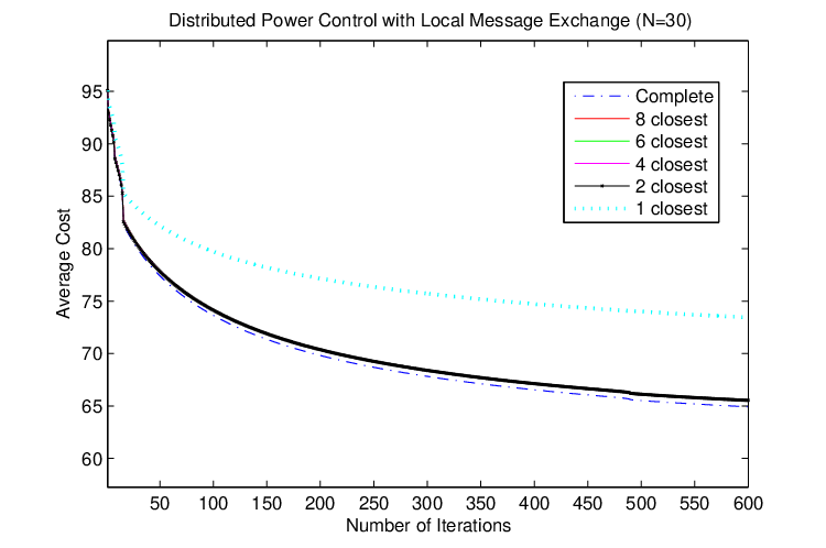
For example, the dotted line represents the cost trajectory generated by the PC algorithm that approximates the marginal cost $\delta\gamma_{i}$ using $MSG(j)$ only from the node nearest to $i$ . Results from Figure 7 indicate that as long as the computation of $\delta\gamma_{i}$ incorporates messages from at least two nearest neighbors, the performance of PC is almost indistinguishable from that of PC with complete message exchange.

VIII-D Algorithms with Delayed and Noisy Messages

Finally, we simulate the joint application of the routing, power allocation, and power control algorithms in the presence of delay and noise in the exchange of marginal cost messages. We model the delay resulting from infrequent updates by the nodes. Specifically, we let each node $i$ update routing message $\frac{\partial D}{\partial r_{i}(w)}$ using (26) only when it iterates $RT(\boldsymbol{\phi}_{i}(w))$ , and we let node $i$ update power control message $MSG(i)$ using (58) only when it iterates $PC(\gamma_{i})$ . As a consequence, the marginal costs $\delta\phi_{ij}(w)$ and $\gamma_{i}$ have to be computed based on outdated information from other nodes, as that information was last updated when the other nodes last iterated.

In addition to delay, we assume messages are subject to noise such that the message received is a random factor times the true value.¹⁹¹⁹ 19 The multiplicative noise is attributed to, for instance, errors in estimating the state of the fading channel over which marginal cost messages are sent. Each message transmission is subject to an independent random factor drawn from a uniform distribution on $[1-\textrm{NoiseScale},1+\textrm{NoiseScale}]$ where the parameter NoiseScale is taken to be $0.9$ in the simulations shown in Figure 8.

Compared to using constantly updated and noiseless messages, the algorithms with delayed and noisy message exchange converge to a limit only slightly worse than the true optimum.

In conclusion, the simulation results confirm that the BRT, BPA and PC algorithms have fast and guaranteed convergence. Moreover, they exhibit satisfactory convergence behavior under changing network topology and traffic demands, as well as in the presence of delay and noise in the marginal cost exchange process. In particular, the PC algorithm performs reasonably well when power control messages are propagated only locally. All these results attest to the practical applicability of our algorithms to real wireless networks.

Finally, we note that the power allocation and power control accounted for most of the cost reduction when the performance of RT with BPA and PC was compared to that of AODV with BPA and PC. This points to the importance of jointly optimizing power control and routing, and suggests that implementing the power allocation and power control algorithms jointly with existing routing algorithms can result in large performance gains.

IX Conclusion

We have presented a general flow-based analytical framework in which power control, rate allocation, routing, and congestion control can be jointly optimized to balance aggregate user utility and total network cost in wireless networks. A complete set of distributed node-based scaled gradient projection algorithms are developed for interference-limited networks where routing, power allocation, and power control variables are iteratively adjusted at individual nodes. We have explicitly characterized the appropriate scaling matrices under which the distributed algorithms converge to the global optimum from any initial point with finite cost. It is shown that the computation of these scaling matrices require only a limited number of control message exchanges in the network. Moreover, convergence does not depend on any particular ordering and synchronization in implementing the algorithms at different nodes.

To enlarge the space of feasible controls, we relaxed the high-SINR assumption for SINR-dependent link models by using the precise capacity function for the problem of jointly optimizing routing and power allocation. We further extended the analytical framework to consider wireless networks with general convex capacity region and strictly quasiconvex link costs. It is proved that in this general setting, an operating point satisfying equilibrium conditions is Pareto optimal. Next, we showed that congestion control can be seamlessly incorporated into our framework, in the sense that the problem of jointly optimal power control, routing, and congestion control can be made equivalent to a problem involving power control and routing in a virtual wireless network with the addition of virtual overflow links. Finally, results from numerical experiments indicate that the distributed network algorithms have superior performance relative to existing schemes, that the algorithms have good adaptability to time-varying network conditions, and that they are robust to delay and noise in the control message exchange process.

-A Proof of Lemma 1

Multiplying both sides of (26) for $i=O(w)$ by $r_{w}$ and summing over all $w\in{\cal W}$ , we have

$\displaystyle\displaystyle{\sum_{w\in{\cal W}}\frac{\partial D}{\partial r_{O(w)}(w)}\cdot r_{w}}$	$\displaystyle=$	$\displaystyle\displaystyle{\sum_{w\in{\cal W}}\sum\limits_{k\in{\cal O}(O(w))}r_{w}\phi_{O(w)k}(w)\left[\frac{\partial D_{O(w)k}}{\partial F_{O(w)k}}(C_{O(w)k},F_{O(w)k})+\frac{\partial D}{\partial r_{k}(w)}\right]}$
	$\displaystyle=$	$\displaystyle\displaystyle{\sum_{w\in{\cal W}}\sum_{k\in{\cal O}(O(w))}f_{O(w)k}(w)\frac{\partial D_{O(w)k}}{\partial F_{O(w)k}}(C_{O(w)k},F_{O(w)k})}$
		$\displaystyle+\displaystyle{\sum_{w\in{\cal W}}\sum_{k\in{\cal O}(O(w))}\sum_{j\in{\cal O}(k)}f_{O(w)k}(w)\phi_{kj}(w)\left[\frac{\partial D_{kj}}{\partial F_{kj}}(C_{kj},F_{kj})+\frac{\partial D}{\partial r_{j}(w)}\right]}.$

Expand the term $\frac{\partial D}{\partial r_{j}(w)}$ repeatedly until $j=D(w)$ , where $\frac{\partial D}{\partial r_{j}(w)}=0$ . Then, use the flow conservation relation $t_{k}(w)=\sum_{i\in{\cal I}(k)}f_{ik}(w)$ for $k\neq O(w)$ to successively factor out terms $t_{k}(w)\phi_{kj}(w)=f_{kj}(w)$ . Finally, noticing that the outermost summation yields

F_{ik}=\sum_{w\in{\cal W}}{f_{ik}(w)},

we obtain the equality of the LHS and RHS of (36). ∎

-B Proof of Lemma 2

For simplicity, we suppress session index $w$ and iteration index $k$ . For $i\neq D(w)$ , the entries of $H_{\boldsymbol{\phi}_{i}}^{\lambda}$ corresponding to subspace $\left\{\boldsymbol{v}_{i}:\sum_{j\in{\cal AN}_{i}}{v_{ij}}=0\right\}$ are as follows. For $k,j\in{\cal AN}_{i}$ ,

\begin{array}[]{l}\vskip 2.84526pt\displaystyle{\left[H_{\boldsymbol{\phi}_{i}}^{\lambda}\right]_{kk}=\frac{\partial^{2}D}{\partial\phi_{ik}^{2}}=t_{i}^{2}\left[\frac{\partial^{2}D_{ik}}{\partial F_{ik}^{2}}+\frac{\partial^{2}D}{\partial r_{k}^{2}}\right]},\\ \vskip 2.84526pt\displaystyle{\left[H_{\boldsymbol{\phi}_{i}}^{\lambda}\right]_{kj}=\frac{\partial^{2}D}{\partial\phi_{ik}\partial\phi_{ij}}=t_{i}^{2}\frac{\partial^{2}D}{\partial r_{k}\partial r_{j}}},\;k\neq j.\end{array}

(87)

Note that the terms $\frac{\partial^{2}D_{ik}}{\partial F_{ik}^{2}}$ are locally measurable. Thus, in the following, we deal only with the terms $\frac{\partial^{2}D}{\partial r_{k}^{2}}$ and $\frac{\partial^{2}D}{\partial r_{k}\partial r_{j}}$ for $k,j\in{\cal AN}_{i}$ . In [3], the authors provide the following useful expression:

\frac{\partial^{2}D}{\partial r_{k}\partial r_{j}}=\sum_{(m,n)\in{\cal E}}{q_{mn}(k)q_{mn}(j)\frac{\partial^{2}D_{mn}}{\partial F_{mn}^{2}}},

(88)

where $q_{mn}(k)$ denotes the fraction of a unit flow originating at node $k$ that goes through link $(m,n)$ . By the Cauchy-Schwarz Inequality,

\frac{\partial^{2}D}{\partial r_{k}\partial r_{j}}\leq\sqrt{\frac{\partial^{2}D}{\partial r_{k}^{2}}\frac{\partial^{2}D}{\partial r_{j}^{2}}}.

(89)

Multiplying $H_{\boldsymbol{\phi}_{i}}^{\lambda}$ on the left and right with non-zero vector $\boldsymbol{v}_{i}$ , we have

\begin{array}[]{ll}\vskip 2.84526pt\boldsymbol{v}_{i}^{\prime}\cdot H^{\lambda}_{\boldsymbol{\phi}_{i}}\cdot\boldsymbol{v}_{i}&\displaystyle{=t_{i}^{2}\left[\sum_{j\in{\cal AN}_{i}}{\left(\frac{\partial^{2}D_{ij}}{\partial F_{ij}^{2}}+\frac{\partial^{2}D}{\partial r_{j}^{2}}\right)v_{ij}^{2}}+\sum_{\scriptstyle j,k\in{\cal AN}_{i}\hfill\atop\scriptstyle{\textrm{and}}~j\neq k\hfill}{\frac{\partial^{2}D}{\partial r_{j}\partial r_{k}}v_{ij}v_{ik}}\right]}\\ &\displaystyle{\leq t_{i}^{2}\left[\sum_{j\in{\cal AN}_{i}}{\left(\frac{\partial^{2}D_{ij}}{\partial F_{ij}^{2}}+\frac{\partial^{2}D}{\partial r_{j}^{2}}\right)v_{ij}^{2}}+\sum_{\scriptstyle j,k\in{\cal AN}_{i}\hfill\atop\scriptstyle{\textrm{and}}~j\neq k\hfill}{\sqrt{\frac{\partial^{2}D}{\partial r_{j}^{2}}\frac{\partial^{2}D}{\partial r_{k}^{2}}}|v_{ij}||v_{ik}|}\right]}\\ &\displaystyle{=t_{i}^{2}\left[\sum_{j\in{\cal AN}_{i}}{\frac{\partial^{2}D_{ij}}{\partial F_{ij}^{2}}v_{ij}^{2}}+\left(\sum_{j\in{\cal AN}(i)}{\sqrt{\frac{\partial^{2}D}{\partial r_{j}^{2}}}|v_{ij}|}\right)^{2}\right]}\\ &\displaystyle{\leq t_{i}^{2}\left[\sum_{j\in{\cal AN}_{i}}{\left(\frac{\partial^{2}D_{ij}}{\partial F_{ij}^{2}}+|{\cal AN}_{i}|\frac{\partial^{2}D}{\partial r_{j}^{2}}\right)v_{ij}^{2}}\right]}\\ &=t_{i}^{2}\cdot\boldsymbol{v}_{i}^{\prime}\cdot\tilde{H}_{\boldsymbol{\phi}_{i}}\cdot\boldsymbol{v}_{i},\end{array}

(90)

where the last inequality follows from applying the Cauchy-Schwarz Inequality to the inner product of vector $(\sqrt{\frac{\partial^{2}D}{\partial r_{j}^{2}}}|v_{ij}|)_{j\in{\cal AN}_{i}}$ with the all-one vector of the same dimension. Thus, the Hessian matrix is upper bounded by the positive definite matrix $t_{i}^{2}\cdot\tilde{H}_{\boldsymbol{\phi}_{i}}$ , where

\tilde{H}_{\boldsymbol{\phi}_{i}}={\rm diag}\left\{\frac{\partial^{2}D_{ij}}{\partial F_{ij}^{2}}+|{\cal AN}_{i}|\frac{\partial^{2}D}{\partial r_{j}^{2}}\right\}_{j\in{\cal AN}_{i}}.

Note that $|{\cal AN}_{i}|$ is the non-blocked out-degree of node $i$ at the current iteration. Also, note that $\frac{\partial^{2}D_{ij}}{\partial F_{ij}^{2}}$ and $\frac{\partial^{2}D}{\partial r_{j}^{2}}$ are evaluated at $\lambda\boldsymbol{\phi}_{i}^{k}+(1-\lambda)\boldsymbol{\phi}_{i}^{k+1}\triangleq\boldsymbol{\phi}_{i}^{k,\lambda}$ for some $\lambda\in[0,1]$ .

There are various ways of producing approximate upper bounds on the diagonal terms in $\tilde{H}_{\boldsymbol{\phi}_{i}}$ . Bertsekas et al.[3] propose a message propagation scheme in the network where the propagated messages are upper bounds of $\frac{\partial^{2}D}{\partial r_{j}^{2}}$ calculated by the corresponding nodes using the bounds provided by their downstream nodes. Such information exchange can be implemented in the same manner as that used for propagating the first derivative cost information $\frac{\partial D}{\partial r_{j}(w)}$ .

To limit communication and computational complexity in wireless networks, we present another scheme which requires less overhead but nevertheless yields reasonable bounds. Let $A\triangleq\max_{(m,n)\in{\cal E}}\left.\frac{\partial^{2}D_{mn}}{\partial F_{mn}^{2}}\right|_{F_{mn}=F_{mn}(\boldsymbol{\phi}_{i}^{k,\lambda})}$ . We have

\frac{\partial^{2}D}{\partial r_{j}^{2}}=\sum_{(m,n)}q_{mn}(j)^{2}\left.\frac{\partial^{2}D_{mn}}{\partial F_{mn}^{2}}\right|_{F_{mn}=F_{mn}(\boldsymbol{\phi}_{i}^{k,\lambda})}\leq A\sum_{(m,n)}q_{mn}(j)^{2}\leq A\sum_{(m,n)}q_{mn}(j)\leq A\cdot h_{j}.

To prove the last inequality, we focus on paths connecting $j$ and $D(w)$ induced by any loop-free routing pattern. Denote the collection of such paths by ${\cal P}_{j}$ and let $\delta_{p}$ be the increase of path flow on $p\in{\cal P}_{j}$ as the result of a unit increment of input at node $j$ . Thus, we have $\sum_{p\in{\cal P}_{j}}\delta_{p}=1$ and

q_{mn}(j)=\sum_{p\in{\cal P}_{j}:(m,n)\in p}\delta_{p}.

Summing over all $(m,n)$ , we obtain

\sum_{(m,n)}q_{mn}(j)=\sum_{(m,n)}\sum_{p\in{\cal P}_{j}:(m,n)\in p}\delta_{p}=\sum_{p\in{\cal P}_{j}}\sum_{(m,n)\in p}\delta_{p}=\sum_{p\in{\cal P}_{j}}h_{j}(p)\cdot\delta_{p}\leq h_{j},

where $h_{j}(p)$ is the number of hops on path $p$ and $h_{j}=\max_{p\in{\cal P}_{j}}h_{j}(p)$ .

Now since the initial network cost is no greater than $D^{0}$ and the cost is strictly reduced with every iteration of $RT(\cdot)$ until conditions (31)-(32) are satisfied, for two consecutive steps $k$ and $k+1$ , on any link $(m,n)$ , $\left.D_{mn}(C_{mn},F_{mn})\right|_{F_{mn}=F_{mn}(\boldsymbol{\phi}_{i}^{k})}\leq D^{0}$ and $\left.D_{mn}(C_{mn},F_{mn})\right|_{F_{mn}=F_{mn}(\boldsymbol{\phi}_{i}^{k+1})}\leq D^{0}$ . By convexity of the cost function, $\left.D_{mn}(C_{mn},F_{mn})\right|_{F_{mn}=F_{mn}(\boldsymbol{\phi}_{i}^{k,\lambda})}\leq D^{0}$ , for all $\lambda\in[0,1]$ . Therefore by the definitions of $A(D^{0})$ and $A$ , we have $A\leq A(D^{0})$ . Also $\left.\frac{\partial^{2}D_{ij}}{\partial F_{ij}^{2}}\right|_{F_{ij}=F_{ij}(\boldsymbol{\phi}_{i}^{k,\lambda})}\leq A_{ij}(D^{0})$ for the same reason. Putting all these results together, we can further upper bound $t_{i}^{2}\cdot\tilde{H}_{\boldsymbol{\phi}_{i}}$ by

{t_{i}}^{2}{\rm diag}\left\{\left(A_{ij}(D^{0})+|{\cal AN}_{i}|h_{j}A(D_{0})\right)_{j\in{\cal AN}_{i}}\right\}.

Thus, the proof is complete. ∎

-C Proof of Lemma 3

Constrained in ${\cal V}_{\boldsymbol{\eta}_{i}}$ , the transmission powers, hence the capacities, of node $i$ ’s outgoing links are subject to change. We can therefore focus on $C_{ij}$ for $j\in{\cal O}(i)$ and take it as a function of $\eta_{ij}$ :

C_{ij}=C(SINR_{ij})=C\left(\frac{G_{ij}P_{i}\eta_{ij}}{G_{ij}P_{i}(1-\eta_{ij})+\sum_{m\neq i}G_{mj}P_{m}+N_{j}}\right)\triangleq C_{ij}(\eta_{ij}).

It can be seen that the Hessian matrix $H_{\boldsymbol{\eta}_{i}}^{k,\lambda}$ is diagonal. Omitting the superscript $(k,\lambda)$ , we can write the diagonal terms as

	$\displaystyle\left[H_{\boldsymbol{\eta}_{i}}\right]_{jj}$	$\displaystyle=$	$\displaystyle\frac{\partial^{2}D_{ij}}{\partial C_{ij}^{2}}\left[C^{\prime}(x_{ij})\frac{G_{ij}P_{i}}{IN_{ij}}(1+x_{ij})\right]^{2}+\frac{\partial D_{ij}}{\partial C_{ij}}\left[C^{\prime\prime}(x_{ij})\left(\frac{G_{ij}P_{i}}{IN_{ij}}(1+x_{ij})\right)^{2}+C^{\prime}(x_{ij})\frac{G_{ij}^{2}P_{i}^{2}}{IN_{ij}^{2}}(2+2x_{ij})\right]$
		$\displaystyle=$	$\displaystyle\left(\frac{P_{i}}{P_{ij}}\right)^{2}\left\{\frac{\partial^{2}D_{ij}}{\partial C_{ij}^{2}}C^{\prime}(x_{ij})^{2}x_{ij}^{2}(1+x_{ij})^{2}+\frac{\partial D_{ij}}{\partial C_{ij}}\left[C^{\prime\prime}(x_{ij})x_{ij}^{2}(1+x_{ij})^{2}+2C^{\prime}(x_{ij})x_{ij}^{2}(1+x_{ij})\right]\right\}.$

Because $\eta_{ij}$ must be lower bounded by $\underline{\eta}_{ij}>0$ for which $D_{ij}(C_{ij}(\underline{\eta}_{ij}),F_{ij}^{k})=D_{i}^{k}$ , we have $\eta_{ij}^{k,\lambda}>\underline{\eta}_{ij}$ and $x_{ij}^{k,\lambda}$ is bounded as

x_{ij}^{min}=\frac{G_{ij}P_{i}\underline{\eta}_{ij}}{G_{ij}P_{i}(1-\underline{\eta}_{ij})+\sum_{m\neq i}G_{mj}P_{m}+N_{j}}\leq x_{ij}^{k,\lambda}\leq\frac{G_{ij}P_{i}}{\sum_{m\neq i}G_{mj}P_{m}+N_{j}}=x_{ij}^{max},

Thus, by dropping the negative term $2\frac{\partial D_{ij}}{\partial C_{ij}}C^{\prime}(x_{ij})x_{ij}^{2}(1+x_{ij})$ and recalling the definition of $\beta_{ij}$ in (51), the diagonal term can be bounded as

	$\displaystyle\left[H_{\boldsymbol{\eta}_{i}}\right]_{jj}$	$\displaystyle\leq$	$\displaystyle\left(\frac{1}{\eta_{ij}^{k,\lambda}}\right)^{2}\left[\frac{\partial^{2}D_{ij}}{\partial C_{ij}^{2}}\max_{x_{ij}^{min}\leq x\leq x_{ij}^{max}}\{C^{\prime}(x)^{2}x^{2}(1+x)^{2}\}+\frac{\partial D_{ij}}{\partial C_{ij}}\min_{x_{ij}^{min}\leq x\leq x_{ij}^{max}}\{C^{\prime\prime}(x)x^{2}(1+x)^{2}\}\right]$
		$\displaystyle<$	$\displaystyle\beta_{ij}.$

Therefore, the lemma follows. ∎

-D Proof of Lemma 4

For brevity, we suppress the superscript $(k,\lambda)$ wherever it arises. The Hessian matrix under consideration has diagonal terms

$\displaystyle[H_{\boldsymbol{\gamma}}]_{ii}$	$\displaystyle=$	$\displaystyle\frac{\partial^{2}D}{\partial\gamma_{i}^{2}}$
	$\displaystyle=$	$\displaystyle\bar{S}_{i}^{2}\left\{\sum_{m\neq i}\sum_{j\in{\cal O}(m)}\frac{\partial^{2}D_{mj}}{\partial C_{mj}^{2}}(C^{\prime}_{mj})^{2}x_{mj}^{2}\left(\frac{G_{ij}P_{i}}{IN_{mj}}\right)^{2}+\frac{\partial D_{mj}}{\partial C_{mj}}(C_{mj}^{\prime\prime}x_{mj}^{2}+2C_{mj}^{\prime}x_{mj})\left(\frac{G_{ij}P_{i}}{IN_{mj}}\right)^{2}\right.$
		$\displaystyle-\frac{\partial D_{mj}}{\partial C_{mj}}C_{mj}^{\prime}x_{mj}\frac{G_{ij}P_{i}}{IN_{mj}}+\sum_{j\in{\cal O}(i)}\frac{\partial^{2}D_{ij}}{\partial C_{ij}^{2}}C_{ij}^{\prime 2}x_{ij}^{2}\left(1-\frac{G_{ij}(1-\eta_{ij})P_{i}}{IN_{ij}}\right)^{2}$
		$\displaystyle+\frac{\partial D_{ij}}{\partial C_{ij}}\left[(C_{ij}^{\prime\prime}x_{ij}^{2}+C_{ij}^{\prime}x_{ij})\left(1-\frac{G_{ij}(1-\eta_{ij})P_{i}}{IN_{ij}}\right)^{2}+C_{ij}^{\prime}x_{ij}\left(\frac{G_{ij}(1-\eta_{ij})P_{i}}{IN_{ij}}\right)^{2}\right.$
		$\displaystyle\left.\left.-C_{ij}^{\prime}x_{ij}\frac{G_{ij}(1-\eta_{ij})P_{i}}{IN_{ij}}\right]\right\}$
	$\displaystyle<$	$\displaystyle\bar{S}_{i}^{2}\left\{\sum_{m\neq i}\sum_{j\in{\cal O}(m)}\frac{\partial^{2}D_{mj}}{\partial C_{mj}^{2}}(C^{\prime}_{mj})^{2}x_{mj}^{2}\left(\frac{G_{ij}P_{i}}{IN_{mj}}\right)^{2}+\frac{\partial D_{mj}}{\partial C_{mj}}(C_{mj}^{\prime\prime}x_{mj}^{2}+2C_{mj}^{\prime}x_{mj})\left(\frac{G_{ij}P_{i}}{IN_{mj}}\right)^{2}\right.$
		$\displaystyle+\sum_{j\in{\cal O}(i)}\frac{\partial^{2}D_{ij}}{\partial C_{ij}^{2}}C_{ij}^{\prime 2}x_{ij}^{2}\left(1-\frac{G_{ij}(1-\eta_{ij})P_{i}}{IN_{ij}}\right)^{2}$
		$\displaystyle+\frac{\partial D_{ij}}{\partial C_{ij}}\left[(C_{ij}^{\prime\prime}x_{ij}^{2}+C_{ij}^{\prime}x_{ij})\left(1-\frac{G_{ij}(1-\eta_{ij})P_{i}}{IN_{ij}}\right)^{2}+C_{ij}^{\prime}x_{ij}\left(\frac{G_{ij}(1-\eta_{ij})P_{i}}{IN_{ij}}\right)^{2}\right]$
		$\displaystyle\left.-\sum_{(m,j)\in{\cal E}}\frac{\partial D_{mj}}{\partial C_{mj}}C_{mj}^{\prime}x_{mj}\right\}.$

The off-diagonal terms of the Hessian are

$\displaystyle\left[H_{\boldsymbol{\gamma}}\right]_{il}$	$\displaystyle=$	$\displaystyle\frac{\partial^{2}D}{\partial\gamma_{i}\partial\gamma_{l}}$
	$\displaystyle=$	$\displaystyle\bar{S}_{i}\bar{S}_{l}\left\{\sum_{j\in{\cal O}(i)}\frac{\partial^{2}D_{ij}}{\partial C_{ij}^{2}}(C^{\prime}_{ij})^{2}x_{ij}^{2}\left(1-\frac{G_{ij}(1-\eta_{ij})P_{i}}{IN_{ij}}\right)\frac{-G_{lj}P_{l}}{IN_{ij}}\right.$
		$\displaystyle+\frac{\partial D_{ij}}{\partial C_{ij}}\left[(C_{ij}^{\prime\prime}x_{ij}^{2}+C_{ij}^{\prime}x_{ij})\left(1-\frac{G_{ij}(1-\eta_{ij})P_{i}}{IN_{ij}}\right)\frac{-G_{lj}P_{l}}{IN_{ij}}+(C_{ij}^{\prime}x_{ij})\frac{G_{ij}G_{lj}(1-\eta_{ij})P_{i}P_{l}}{IN_{ij}^{2}}\right]$
		$\displaystyle+\sum_{j\in{\cal O}(l)}\frac{\partial^{2}D_{lj}}{\partial C_{lj}^{2}}(C^{\prime}_{lj})^{2}x_{lj}^{2}\left(1-\frac{G_{lj}(1-\eta_{lj})P_{l}}{IN_{lj}}\right)\frac{-G_{ij}P_{i}}{IN_{lj}}$
		$\displaystyle+\frac{\partial D_{lj}}{\partial C_{lj}}\left[(C_{lj}^{\prime\prime}x_{lj}^{2}+C_{lj}^{\prime}x_{lj})\left(1-\frac{G_{lj}(1-\eta_{lj})P_{l}}{IN_{lj}}\right)\frac{-G_{ij}P_{i}}{IN_{lj}}+(C_{lj}^{\prime}x_{lj})\frac{G_{lj}G_{ij}(1-\eta_{lj})P_{l}P_{i}}{IN_{lj}^{2}}\right]$
		$\displaystyle\left.+\sum_{m\neq i,l}{\sum_{j\in{\cal O}(m)}\frac{\partial^{2}D_{mj}}{\partial C_{mj}^{2}}(C^{\prime}_{mj})^{2}x_{mj}^{2}\frac{G_{ij}P_{i}G_{lj}P_{l}}{IN_{mj}^{2}}+\frac{\partial D_{mj}}{\partial C_{mj}}(C_{mj}^{\prime\prime}x_{mj}^{2}+2C_{mj}^{\prime}x_{mj})\frac{G_{ij}P_{i}G_{lj}P_{l}}{IN_{mj}^{2}}}\right\}.$

Construct the following vectors for each $i\in{\cal N}$ .

U_{i}\triangleq\left\{\begin{array}[]{ll}\vskip 2.84526pt[U_{i}]_{(m,j)}=\displaystyle{\sqrt{\frac{\partial^{2}D_{mj}}{\partial C_{mj}^{2}}}C_{mj}^{\prime}x_{mj}\frac{G_{ij}P_{i}}{IN_{mj}}\bar{S}_{i}v_{i}},&\forall m\neq i~\textrm{and}~j\in{\cal O}(m)\\ \vskip 2.84526pt[U_{i}]_{(i,j)}=\displaystyle{-\sqrt{\frac{\partial^{2}D_{ij}}{\partial C_{ij}^{2}}}C_{ij}^{\prime}x_{ij}\left(1-\frac{G_{ij}(1-\eta_{ij})P_{i}}{IN_{ij}}\right)\bar{S}_{i}v_{i}},&\forall j\in{\cal O}(i)\end{array}\right.

and

T_{i}\triangleq\left\{\begin{array}[]{ll}\vskip 2.84526pt[T_{i}]_{(m,j)}=\displaystyle{\sqrt{-\frac{\partial D_{mj}}{\partial C_{mj}}C_{mj}^{\prime}x_{mj}}\frac{G_{ij}P_{i}}{IN_{mj}}\bar{S}_{i}v_{i}},&\forall m\neq i~\textrm{and}~j\in{\cal O}(m)\\ \vskip 2.84526pt[T_{i}]_{(i,j)}=\displaystyle{\sqrt{-\frac{\partial D_{ij}}{\partial C_{ij}}C_{ij}^{\prime}x_{ij}}\frac{G_{ij}(1-\eta_{ij})P_{i}}{IN_{ij}}\bar{S}_{i}v_{i}},&\forall j\in{\cal O}(i)\end{array}\right..

W_{i}\triangleq\left\{\begin{array}[]{ll}\vskip 2.84526pt[W_{i}]_{(m,j)}=\displaystyle{\sqrt{\frac{\partial D_{mj}}{\partial C_{mj}}(C^{\prime\prime}_{mj}x_{mj}^{2}+C_{mj}^{\prime}x_{mj})}\frac{G_{ij}P_{i}}{IN_{mj}}\bar{S}_{i}v_{i}},&\forall m\neq i~\textrm{and}~j\in{\cal O}(m)\\ \vskip 2.84526pt[W_{i}]_{(i,j)}=\displaystyle{-\sqrt{\frac{\partial D_{ij}}{\partial C_{ij}}(C^{\prime\prime}_{ij}x_{ij}^{2}+C_{ij}^{\prime}x_{ij})}\left(1-\frac{G_{ij}(1-\eta_{ij})P_{i}}{IN_{ij}}\right)\bar{S}_{i}v_{i}},&\forall j\in{\cal O}(i)\end{array}\right..

Thus, for any nonzero vector $\boldsymbol{v}\in\mathbb{R}^{|{\cal N}|}$ we have

			$\displaystyle\boldsymbol{v}^{\prime}\cdot H_{\boldsymbol{\gamma}}\cdot\boldsymbol{v}$
		$\displaystyle<$	$\displaystyle\sum_{i,l\in{\cal N}}{U_{i}^{\prime}\cdot U_{l}}+\sum_{i,l\in{\cal N}}{W_{i}^{\prime}\cdot W_{l}}-\sum_{i,l\in{\cal N}}{T_{i}^{\prime}\cdot T_{l}}+\sum_{i\in{\cal N}}{\sum_{(m,j)\in{\cal E}}{-\frac{\partial D_{mj}}{\partial C_{mj}}C_{mj}^{\prime}x_{mj}\bar{S}_{i}^{2}v_{i}^{2}}}$
		$\displaystyle\leq$	$\displaystyle\sum_{i,l\in{\cal N}}{\\|U_{i}\\|\cdot\\|U_{l}\\|}+\sum_{i,l\in{\cal N}}{\\|W_{i}\\|\cdot\\|W_{l}\\|}+\sum_{i\in{\cal N}}{\sum_{(m,j)\in{\cal E}}{-\frac{\partial D_{mj}}{\partial C_{mj}}C_{mj}^{\prime}x_{mj}\bar{S}_{i}^{2}v_{i}^{2}}}$
		$\displaystyle\leq$	$\displaystyle\frac{1}{2}\sum_{i,l\in{\cal N}}{\left(\\|U_{i}\\|^{2}+\\|U_{l}\\|^{2}+\\|W_{i}\\|^{2}+\\|W_{l}\\|^{2}\right)}+\sum_{i\in{\cal N}}{\sum_{(m,j)\in{\cal E}}{-\frac{\partial D_{mj}}{\partial C_{mj}}C_{mj}^{\prime}x_{mj}\bar{S}_{i}^{2}v_{i}^{2}}}$
		$\displaystyle=$	$\displaystyle\|{\cal N}\|\sum_{i\in{\cal N}}\left(\\|U_{i}\\|^{2}+\\|W_{i}\\|^{2}\right)+\sum_{i\in{\cal N}}{\sum_{(m,j)\in{\cal E}}{-\frac{\partial D_{mj}}{\partial C_{mj}}C_{mj}^{\prime}x_{mj}\bar{S}_{i}^{2}v_{i}^{2}}}$
		$\displaystyle=$	$\displaystyle\sum_{i\in{\cal N}}v_{i}^{2}\bar{S}_{i}^{2}\left\{\|{\cal N}\|\left[\sum_{j\in{\cal O}(i)}\left(\frac{\partial^{2}D_{ij}}{\partial C_{ij}^{2}}(C^{\prime}_{ij})^{2}x_{ij}^{2}+\frac{\partial D_{ij}}{\partial C_{ij}}(C^{\prime\prime}_{ij}x_{ij}^{2}+C^{\prime}_{ij}x_{ij})\right)\left(1-\frac{G_{ij}(1-\eta_{ij})P_{i}}{IN_{ij}}\right)^{2}\right.\right.$
			$\displaystyle\left.+\sum_{m\neq i}{\sum_{j\in{\cal O}_{m}}\left(\frac{\partial^{2}D_{mj}}{\partial C_{mj}^{2}}(C^{\prime}_{mj})^{2}x_{mj}^{2}+\frac{\partial D_{mj}}{\partial C_{mj}}(C^{\prime\prime}_{mj}x_{mj}^{2}+C^{\prime}_{mj}x_{mj})\right)\left(\frac{G_{ij}P_{i}}{IN_{mj}}\right)^{2}}\right]$
			$\displaystyle+\left.\sum_{(m,j)\in{\cal E}}-\frac{\partial D_{mj}}{\partial C_{mj}}C^{\prime}_{mj}x_{mj}\right\}.$

To get a simpler upper bound, notice that $\left(1-\frac{G_{ij}(1-\eta_{ij})P_{i}}{IN_{ij}}\right)^{2}\leq 1$ , $\left(\frac{G_{ij}P_{i}}{IN_{mj}}\right)^{2}<1$ , and by assumption $\frac{\partial D_{mj}}{\partial C_{mj}}<0$ , $C^{\prime\prime}_{mj}x_{mj}^{2}+C^{\prime}_{mj}x_{mj}\leq 0$ , the whole summation in the curly bracket can be bounded by

|{\cal N}|\left(\sum_{(m,j)\in{\cal E}}\frac{\partial^{2}D_{mj}}{\partial C_{mj}^{2}}(C^{\prime}_{mj})^{2}x_{mj}^{2}+\frac{\partial D_{mj}}{\partial C_{mj}}C^{\prime\prime}_{mj}x_{mj}^{2}\right).

Due to the peak power constraint, there exists a global upper bound on the achievable $SINR$ on all links, that is $\bar{x}\geq\max_{(m,j)\in{\cal E}}x_{mj}$ . Recall the definitions for $\kappa$ , $\varphi$ , $\bar{B}(D^{0})$ , and $\underline{B}(D^{0})$ : $\kappa=\max_{0\leq x\leq\bar{x}}(C^{\prime}(x))^{2}\cdot x^{2}$ , $\varphi=\min_{0\leq x\leq\bar{x}}C^{\prime\prime}(x)\cdot x^{2}$ ,

\bar{B}(D^{0})=\max_{(m,j)\in{\cal E}}\max_{D_{mj}\leq D^{0}}\frac{\partial^{2}D_{mj}}{\partial C_{mj}^{2}},

and

\underline{B}(D^{0})=\min_{(m,j)\in{\cal E}}\min_{D_{mj}\leq D^{0}}\frac{\partial D_{mj}}{\partial C_{mj}}.

We obtain

\boldsymbol{v}^{\prime}\cdot H_{\boldsymbol{\gamma}}\cdot\boldsymbol{v}<\sum_{i\in{\cal N}}v_{i}^{2}\bar{S}_{i}^{2}|{\cal N}||{\cal E}|\left[\bar{B}(D^{0})\kappa+\underline{B}(D^{0})\varphi\right],

i.e., $H_{\boldsymbol{\gamma}}$ is upper bounded by $|{\cal N}||{\cal E}|\left[\bar{B}(D^{0})\kappa+\underline{B}(D^{0})\varphi\right]{\rm diag}\{\left(\bar{S}_{i}^{2}\right)_{i\in{\cal N}}\}$ . ∎

-E Proof of Lemma 6

For convenience, we suppress the index $k$ and parameter $\lambda$ . Using the precise capacity formula (63), we derive the entries the Hessian matrix as

\begin{array}[]{ll}\vskip 2.84526pt\left[H_{\boldsymbol{\eta}_{i}}\right]_{jj}&=\displaystyle{\frac{\partial^{2}D_{ij}}{\partial C_{ij}^{2}}\left(\frac{G_{ij}P_{i}(K-1)}{KG_{ij}P_{ij}+IN_{ij}}+\frac{G_{ij}P_{i}}{IN_{ij}}\right)^{2}+\frac{\partial D_{ij}}{\partial C_{ij}}\left(\frac{-G_{ij}^{2}P_{i}^{2}(K-1)^{2}}{(KG_{ij}P_{ij}+IN_{ij})^{2}}+\frac{G_{ij}^{2}P_{i}^{2}}{IN_{ij}^{2}}\right)}\\ &<\displaystyle{\frac{\partial^{2}D_{ij}}{\partial C_{ij}^{2}}\left[\frac{KG_{ij}P_{i}}{\sum_{m\neq i}G_{mj}P_{m}+N_{j}}\right]^{2}-\frac{\partial D_{ij}}{\partial C_{ij}}\left(\frac{({K-1})G_{ij}P_{i}}{\sum_{m\neq i}G_{mj}P_{m}+N_{j}}\right)^{2}},\\ \left[H_{\boldsymbol{\eta}_{i}}\right]_{lj}&=0,\quad\forall l\neq j.\end{array}

Plugging the expressions (66)-(68), we further bound the diagonal terms of $H_{\boldsymbol{\eta}_{i}}$ as

\left[H_{\boldsymbol{\eta}_{i}}\right]_{jj}<\left[\bar{B}_{ij}(D_{i}^{k})K^{2}-\underline{B}_{ij}(D_{i}^{k})\left({K-1}\right)^{2}\right]NR_{ij}^{2}.

Thus, the proof is complete. ∎

References

[1] D. Cantor and M. Gerla, “Optimal routing in a packet switched computer network,” IEEE Transactions on Comput., vol. C-23, pp. 1062–1069, Oct. 1974.
[2] R. Gallager, “A minimum delay routing algorithm using distributed computation,” IEEE Transactions on Communications, vol. 25, no. 1, pp. 73–85, 1977.
[3] D. Bertsekas, E. Gafni, and R. Gallager, “Second derivative algorithm for minimum delay distributed routing in networks,” IEEE Transactions on Communications, vol. 32, no. 8, pp. 911–919, 1984.
[4] F. P. Kelly, “Charging and rate control for elastic traffic,” European Transactions on Telecommunications, pp. 33–37, 1997.
[5] F. Kelly, A. Maulloo, and D. Tan, “Rate control in communication networks: shadow prices, proportional fairness and stability,” Journal of the Operational Research Society, vol. 49, 1998.
[6] S. Low and D. Lapsley, “Optimization flow control. I. basic algorithm and convergence,” IEEE/ACM Transactions on Networking, vol. 7, pp. 861–874, Dec. 1999.
[7] R. Srikant, The Mathematics of Internet Congestion Control. Birkhauser, 2004.
[8] E. Anderson and T. Anderson, “On the stability of adaptive routing in the presence of congestion control,” in INFOCOM 2003, vol. 2, pp. 948–958, March 2003.
[9] W. Wang, M. Palaniswami, and S. H. Low, “Optimal flow control and routing in multi-path networks,” Performance Evaluation, vol. 52, pp. 119–132, 2003.
[10] X. Lin and N. B. Shroff, “The multi-path utility maximization problem,” in 41st Annual Allerton Conference on Communication, Control and Computing, (Monticello, IL), October 2003.
[11] G. Foschini and Z. Miljanic, “Distributed autonomous wireless channel assignment algorithm with power control,” IEEE Transactions on Vehicular Technology, pp. 420–429, Aug. 1995.
[12] S. Hanly and D. Tse, “Power control and capacity of spread-spectrum wireless networks,” Automatica, vol. 35, pp. 1987–2012, Dec. 1999.
[13] R. Cruz and A. Santhanam, “Optimal link scheduling and power control in CDMA multihop wireless networks,” in IEEE GLOBECOM ’02, pp. 52–56, Nov. 2002.
[14] D. Julian, M. Chiang, and D. O’Neill, “Robust and qos constrained optimization of power control in wireless cellular networks,” in Vehicular Technology Conference, 2001, vol. 3, pp. 1932–1936, Oct. 2001.
[15] R. Cruz and A. Santhanam, “Optimal routing, link scheduling and power control in multihop wireless networks,” in INFOCOM 2003, vol. 1, pp. 702–711, March 2003.
[16] N. Bambos, S. Chen, and G. Pottie, “Channel access algorithms with active link protection for wireless communication networks with power control,” IEEE/ACM Transactions on Networking, vol. 8, pp. 583–597, Oct. 2000.
[17] R. Bhatia and M. Kodialam, “On power efficient communication over multi-hop wireless networks: joint routing, scheduling and power control,” in INFOCOM 2004, vol. 2, pp. 1457–1466, March 2004.
[18] M. Johansson, L. Xiao, and S. Boyd, “Simultaneous routing and power allocation in CDMA wireless data networks,” in Proceedings of IEEE International Conference on Communications, vol. 1, May 2003.
[19] M. Chiang, “To layer or not to layer: Balancing transport and physical layers in wireless multihop networks,” in INFOCOM 2004, vol. 4, Mar. 2004.
[20] C. Perkins and E. Royer, “Ad-hoc on-demand distance vector routing,” in Second IEEE Workshop on Mobile Computing Systems and Applications, Feb. 1999.
[21] D. P. Bertsekas and R. Gallager, Data Networks. Prentice Hall, second ed., 1992.
[22] J. Tsitsiklis and D. Bertsekas, “Distributed asynchronous optimal routing in data networks,” IEEE Transactions on Automatic Control, vol. 31, pp. 325–332, Apr. 1986.
[23] L. Kleinrock, Communication Net: Stochastic Message Flow and Delay. New York: McGraw-Hill, 1964.
[24] K. Kar, S. Sarkar, and L. Tassiulas, “Optimization based rate control for multirate multicast sessions,” in INFOCOM 2001, pp. 123–132, 2001.
[25] A. J. Viterbi, CDMA: Principles of Spread Spectrum Communication. Addison-Wesley Pub. Co., 1995.
[26] D. Tse and P. Viswanath, Fundamentals of Wireless Communication. Cambridge University Press, 2004.
[27] D. P. Bertsekas, Nonlinear Programming. Athena Scientific, 1999.

			$\displaystyle\displaystyle{\sum_{(i,j)\in{\cal E}}{\frac{\partial D_{ij}}{\partial C_{ij}^{}}\sum_{(m,n)\in{\cal E}}{\frac{\partial C_{ij}}{\partial S_{mn}^{}}\cdot(S_{mn}^{1}-S_{mn}^{*})}}}$
		$\displaystyle\stackrel{{\scriptstyle(a)}}{{=}}$	$\displaystyle\sum_{(i,j)\in{\cal E}}\left[-\sum_{(m,n)\in{\cal E}}\frac{\partial D_{mn}}{\partial C_{mn}^{}}(C^{}_{mn})^{\prime}x_{mn}^{}\frac{G_{in}}{IN_{mn}^{}}+\nu_{i}^{}\right]P_{ij}^{}\ln\frac{P_{ij}^{1}}{P_{ij}^{*}}$
		$\displaystyle\stackrel{{\scriptstyle(b)}}{{=}}$	$\displaystyle\sum_{(i,j)\in{\cal E}}\frac{\delta\gamma_{i}^{}}{P_{i}^{}}\cdot P_{ij}^{}\ln\frac{P_{ij}^{1}}{P_{ij}^{}}$
		$\displaystyle\stackrel{{\scriptstyle(c)}}{{\geq}}$	$\displaystyle\displaystyle{\sum_{(i,j)\in{\cal E}}\frac{\delta\gamma_{i}^{}}{P_{i}^{}}\cdot P_{ij}^{}\left(\frac{P_{ij}^{1}}{P_{ij}^{}}-1\right)}$
		$\displaystyle\stackrel{{\scriptstyle(d)}}{{=}}$	$\displaystyle\displaystyle{\sum_{i\in{\cal N}}\frac{\delta\gamma_{i}^{}}{P_{i}^{}}\cdot(P_{i}^{1}-P_{i}^{*})}\stackrel{{\scriptstyle(e)}}{{\geq}}0.$