The Distribution of Patterns in Random TreesThanks: ^∗ INRIA-Rocquencourt, F-78153 Le Chesnay cedex, France, e-mail: frederic.chyzak@inria.frThanks: ^∗∗ Institut für Diskrete Mathematik und Geometrie, Technische Universität Wien, Wiedner Hauptstraße 8-10/113, A-1040 Wien, Austria, e-mail: michael.drmota@tuwien.ac.at, klausner@dmg.tuwien.ac.atThanks: ^∗∗∗ Delft Institute of Applied Mathematics, Delft University of Technology, Mekelweg 4, NL-2628 CD Delft, The Netherlands, e-mail: gkok@fsmat.atThanks: This research was supported by the Austrian Science Foundation FWF, grants S8302 and S9604, and by the European Amadeus project.

Frédéric Chyzak^∗, Michael Drmota^∗∗, Thomas Klausner^∗∗, and Gerard Kok^∗∗∗

Date: August 11, 2026

Abstract.

Let ${\mathcal{T}}_{n}$ denote the set of unrooted labeled trees of size $n$ and let ${\mathcal{M}}$ be a particular (finite, unlabeled) tree. Assuming that every tree of ${\mathcal{T}}_{n}$ is equally likely, it is shown that the limiting distribution as $n$ goes to infinity of the number of occurrences of ${\mathcal{M}}$ as an induced subtree is asymptotically normal with mean value and variance asymptotically equivalent to $\mu n$ and $\sigma^{2}n$ , respectively, where the constants $\mu>0$ and $\sigma\geq 0$ are computable.

1. Introduction

In this paper we consider unrooted labeled trees and analyse the number of occurrences of a tree pattern as an induced subtree of a random tree. It is well known that a typical tree in ${\mathcal{T}}_{n}$ , the set of unrooted labeled trees of size $n$ , has about $\mu_{k}n$ nodes of degree $k$ , where $\mu_{k}=1/e(k-1)!$ . Moreover, for any fixed $k$ the total number of nodes of degree $k$ over all trees in ${\mathcal{T}}_{n}$ satisfies a central limit theorem with mean and variance asymptotically equivalent to $\mu_{k}n$ and $\sigma_{k}^{2}n$ (for a specific constant $\sigma_{k}>0$ ). See [DG99], where Drmota and Gittenberger explored this phenomenon for unrooted labeled trees and other types of trees.

A node of degree $k$ is an occurrence of what can be called a star with $k$ edges. In this paper we continue this idea. We consider a pattern ${\mathcal{M}}$ , a given finite tree, and compute the limiting distribution of the number of occurrences of ${\mathcal{M}}$ in ${\mathcal{T}}_{n}$ as $n\to\infty$ . Note also that there can be overlaps of two or more copies of ${\mathcal{M}}$ , which we intend to count as separate occurrences.

Our main result in this paper is:

Theorem 1.

Let ${\mathcal{M}}$ be a given finite tree. Then the limiting distribution of the number of occurrences of ${\mathcal{M}}$ (as induced subtrees) in a tree of ${\mathcal{T}}_{n}$ is asymptotically normal with mean and variance asymptotically equivalent to $\mu n$ and $\sigma^{2}n$ , respectively, where $\mu>0$ and $\sigma^{2}\geq 0$ depend on the pattern ${\mathcal{M}}$ and can be computed explicitly and algorithmically and can be represented as polynomials (with rational coefficients) in $1/e$ .

We consider here a random variable $X$ as Gaussian if its characteristic function is given by ${\bf E}\,e^{itX}=e^{i\mu t-\sigma^{2}t^{2}/2}$ , that is, the case of zero variance $\sigma^{2}=0$ is included here. For example, if ${\mathcal{M}}$ consists just of one edge (and two nodes), then the number of occurrences of ${\mathcal{M}}$ in ${\mathcal{T}}_{n}$ is $n-1$ and thus constant. So in that particular case we have $\mu=1$ and $\sigma^{2}=0$ . Nevertheless we conjecture that $\sigma^{2}>0$ in all other cases.

As already mentioned, the case of stars (or nodes of given degree) has been discussed in [DG99] for various classes of trees. Some previous work for unlabeled trees is due to Robinson and Schwenk [RS75]. Patterns in (rooted planar) trees have also been considered by Dershowitz and Zaks [DZ89] under the limitation that patterns start at the root. In a work on patterns in random binary search trees, Flajolet, Gourdon, and Martínez [FGM97] obtained a central limit theorem. Flajolet and Steyaert also analysed an algorithm for pattern matchings in trees [FS80a, FS80b, SF83]. Further Ruciǹski [Ruc88] established conditions for when the number of occurrences of a given subgraph in random graphs follows a normal distribution.

The plan of the paper is as follows. In Section 2 we give a short introduction to counting trees with generating functions, and also expand this to two variables for counting stars (nodes of specific degree $k$ ) in trees. In Section 3 we expand this framework to the counting of patterns in trees. The resulting asymptotics are presented in Section 4, concluding the proof of Theorem 1. Technical details for this as well as explicit algorithms can be found in the appendix. In fact, the algorithmic aspect is one of the driving forces of this paper.

2. Counting Trees and Counting Stars in Trees

In this section we introduce a three-step program to count the number of trees in ${\mathcal{T}}_{n}{}$ and in the same fashion the number of occurrences of nodes of degree $k$ in ${\mathcal{T}}_{n}{}$ . While redundant and probably heavy in this simplistic situation, this procedure was crucial to the derivation in [DG99] for counting stars and will generalise well to our setting of general tree patterns.

For this purpose we make use of the sets ${\mathcal{R}}_{n}$ of rooted labeled trees of size $n$ and ${\mathcal{P}}_{n}$ of planted labeled trees of size $n$ . For rooted and unrooted trees, the size $n$ counts the total number of nodes, whether internal or at the leaves. On the other hand, a planted tree is just a rooted tree where the root is adjoined an additional “phantom” node which does not contribute to the size of the tree, whereas the degree of the root is increased by one. As well, one can think of a planted tree as a rooted tree with an additional edge having no end vertex. The advantage of using planted trees, though it seems to add complexity, will be explained below. Obviously $|{\mathcal{P}}_{n}{}|=|{\mathcal{R}}_{n}{}|$ and $|{\mathcal{T}}_{n}{}|=|{\mathcal{R}}_{n}{}|/n$ . It is also well known that $|{\mathcal{R}}_{n}{}|=n^{n-1}$ and $|{\mathcal{T}}_{n}{}|=n^{n-2}$ .

The three-step program is the following one: First, the generating function enumerating planted trees is determined, then it is used to count rooted trees by deriving their generating function, and finally the generating function counting unrooted trees is computed.

We define

p(x)=\sum_{n=0}^{\infty}|{\mathcal{P}}_{n}|\frac{x^{n}}{n!},\quad r(x)=\sum_{n=0}^{\infty}|{\mathcal{R}}_{n}|\frac{x^{n}}{n!},\quad t(x)=\sum_{n=0}^{\infty}|{\mathcal{T}}_{n}|\frac{x^{n}}{n!}

and proceed in the following way:

(1)

Planted Rooted Trees: A planted tree is a planted root node with zero, one, two, $\dots$ planted subtrees of any order. In terms of the generating function this yields

$p(x)=\sum_{n=0}^{\infty}\frac{xp(x)^{n}}{n!}=xe^{p(x)}.$
(2)

Rooted Trees: For rooted trees we get the same (except for the phantom nodes which are not present here), just a root with zero, one, two, $\dots$ planted subtrees of any order

$r(x)=\sum_{n=0}^{\infty}\frac{xp(x)^{n}}{n!}=xe^{p(x)}=p(x).$
(3)

Unrooted Trees: Finally, we have $|{\mathcal{T}}_{n}{}|=|{\mathcal{R}}_{n}{}|/n$ , as already mentioned. However, we can also express $t(x)$ by a relation which follows from a natural bijection between rooted trees on the one hand and unrooted trees and pairs of planted rooted trees (that are joined by identifying the additional edges at their planted roots and discarding the phantom nodes) on the other hand.¹¹ 1 Consider the class of rooted (labeled) trees. If the root is labeled by $1$ then consider the tree as an unrooted tree. If the root is not labeled by $1$ then consider the first edge of the path between the root and $1$ and cut the tree into two planted rooted trees at this edge. This yields

$t(x)=r(x)-\frac{1}{2}p(x)^{2}.$

The functional equation for $p(x)$ can be either used to extract the explicit number $|{\mathcal{P}}_{n}|=n^{n-1}$ via Lagrange inversion or to obtain the radius of convergence and asymptotic expansions of the singular behaviour of this function. It is well known that $x_{0}=1/e$ is the common radius of convergence of $p(x)$ , $r(x)$ , and $t(x)$ , and that the singularity at $x=x_{0}$ is of square-root type:

	$\displaystyle p(x)$	$\displaystyle=r(x)=1-\sqrt{2}\sqrt{1-ex}+\frac{2}{3}(1-ex)+\cdots,$
	$\displaystyle t(x)$	$\displaystyle=\frac{1}{2}-(1-ex)+\frac{2\sqrt{2}}{3}(1-ex)^{3/2}+\cdots.$

This is reflected by the asymptotic expansions of the numbers

	$\displaystyle\|{\mathcal{P}}_{n}{}\|$	$\displaystyle=\|{\mathcal{R}}_{n}{}\|=n^{n-1}\sim\frac{n!}{\sqrt{2\pi}}e^{n}n^{-3/2},$
	$\displaystyle\|{\mathcal{T}}_{n}{}\|$	$\displaystyle=n^{n-2}\sim\frac{n!}{\sqrt{2\pi}}e^{n}n^{-5/2}.$

In order to demonstrate the usefulness of the three-step procedure above we repeat the same steps for counting stars with $k$ edges in trees, that is, the number of nodes of degree $k$ , a given fixed positive number. Let $p_{n,m}$ denote the number of planted trees of size $n$ with exactly $m$ nodes of degree $k$ . Furthermore, let $r_{n,m}$ and $t_{n,m}$ be the corresponding numbers for rooted and unrooted trees and set

p(x,u)=\sum_{n,m=0}^{\infty}p_{n,m}\frac{x^{n}u^{m}}{n!},\quad r(x,u)=\sum_{n,m=0}^{\infty}r_{n,m}\frac{x^{n}u^{m}}{n!},\quad t(x,u)=\sum_{n,m=0}^{\infty}t_{n,m}\frac{x^{n}u^{m}}{n!}.

Then we have (compare with [DG99])

(1)

Planted Rooted Trees:

p(x,u)=\sum_{\begin{subarray}{c}n=0\\ n\neq k-1\end{subarray}}^{\infty}\frac{xp(x,u)^{n}}{n!}+\frac{xup(x,u)^{k-1}}{(k-1)!}=xe^{p(x,u)}+\frac{x(u-1)p(x,u)^{k-1}}{(k-1)!}.

(2)

Rooted Trees:

r(x,u)=\sum_{\begin{subarray}{c}n=0\\ n\neq k\end{subarray}}^{\infty}\frac{xp(x,u)^{n}}{n!}+\frac{xup(x,u)^{k}}{k!}=xe^{p(x,u)}+\frac{x(u-1)p(x,u)^{k}}{k!}.

(3)

Unrooted Trees: Similarly to the above we have $t_{n,m}=r_{n,m}/n$ which is sufficient for our purposes. However, as above, it is also possible to express $t(x,u)$ by

$t(x,u)=r(x,u)-\frac{1}{2}p(x,u)^{2}.$

Note that the use of the notion of planted trees is crucial in order to keep track of the nodes of degree $k$ by means of the recursive structure of planted trees. In [DG99] this approach was used to show that the asymptotic distribution of the number of nodes of degree $k$ in trees of size $n$ is normal, with expectation and variance proportional to $n$ .

3. Counting Patterns in Trees

We now generalize the counting procedure of Section 2 to more complicated patterns. For our purpose, a pattern is a given (finite unrooted unlabeled) tree ${\mathcal{M}}$ . To ease explanations, we will use as ${\mathcal{M}}$ the example graph in Figure 1.

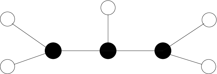
Refer to caption — Figure 1. Example pattern

We say that a specific pattern ${\mathcal{M}}$ occurs in a tree $T$ if ${\mathcal{M}}$ occurs in $T$ as an induced subtree in the sense that the node degrees for the internal (filled) nodes in the pattern match the degrees of the corresponding nodes in $T$ , while the external (empty) nodes match nodes of arbitrary degree.²² 2 More generally we could also consider pattern-matching problems for patterns in which some degrees of certain possibly external “filled” nodes must match exactly while the degrees of the other, possibly internal “empty” nodes might be different. But then the situation is more involved, see Section 5. Because the results for the patterns consisting of only one node or two nodes and one edge are trivial, we now concentrate on patterns with at least three nodes.

Our principal aim is to get relations for the generating functions which count the number of occurrences of a specific pattern ${\mathcal{M}}$ . Let $p_{n,m}$ denote the number of planted rooted trees with $n$ nodes and exactly $m$ occurrences of the pattern ${\mathcal{M}}{}$ and let

p=p(x,u)=\sum_{n,m=0}^{\infty}p_{n,m}\frac{x^{n}u^{m}}{n!}

be the corresponding generating function.

3.1. Generating Functions for Planted Rooted Trees

Proposition 1.

(Planted Rooted Trees) Let ${\mathcal{M}}$ be a pattern. Then there exists a certain number $L+1$ of auxiliary functions $a_{j}(x,u)$ $(0\leq j\leq L)$ with

p(x,u)=\sum_{j=0}^{L}a_{j}(x,u)

and polynomials $P_{j}(y_{0},\ldots,y_{L},u)$ $(1\leq j\leq L)$ with non-negative coefficients such that

(1)	$\displaystyle a_{0}(x,u)$	$\displaystyle=xe^{a_{0}(x,u)+\cdots+a_{L}(x,u)}-x\sum_{j=1}^{L}P_{j}(a_{0}(x,u),\ldots,a_{L}(x,u),1)$
	$\displaystyle a_{1}(x,u)$	$\displaystyle=x\cdot P_{1}(a_{0}(x,u),\ldots,a_{L}(x,u),u)$
		$\displaystyle\vdots$
	$\displaystyle a_{L}(x,u)$	$\displaystyle=x\cdot P_{L}(a_{0}(x,u),\ldots,a_{L}(x,u),u).$

Furthermore,

\sum_{j=1}^{L}P_{j}(y_{0},\ldots,y_{L},1)\leq_{c}e^{y_{0}+\cdots+y_{L}},

where $f\leq_{c}g$ means that all Taylor coefficients of the left-hand side are smaller than or equal to the corresponding coefficients of the right-hand side. Moreover, the dependency graph of this system is strongly connected.³³ 3 The notion of dependency graph is explained in Appendix B and intuitively speaking, reflects the fact that no subsystem can be solved before the whole system.

The proof of this proposition is in fact the core of the paper. In order to make the arguments more transparent we will demonstrate them with the help of the example pattern in Figure 1. At each step of the proof we will also indicate how to make all constructions explicit so that it is possible to generate System (1) effectively.

In a first step we introduce the notion of a planted pattern. A planted pattern ${\mathcal{M}}_{p}$ is just a planted rooted tree where we again distinguish between internal (filled) and external (empty) nodes. It matches a planted rooted tree from ${\mathcal{T}}_{n}$ if ${\mathcal{M}}_{p}$ occurs as an induced subtree starting from the (planted) root, that is, the branch structure and node degrees of the filled nodes match. Two occurrences may overlap. For example, in Figure 2 the planted pattern ${\mathcal{M}}_{p}$ on the left matches the planted tree $A$ twice (following the left, resp. the right edge from the root), but $B$ not at all. Also remark that, notwithstanding the symmetry of $C$ , the pattern ${\mathcal{M}}_{p}$ really matches $C$ twice, as we are interested in matches in labeled trees.

We now construct a planted pattern for each internal (filled) node of our pattern ${\mathcal{M}}$ which is adjacent to an external (empty) node. The internal (filled) node is considered as the planted root and one of the free attached leaves as the plant. In our example we obtain the two graphs in Figure 3.

The next step is to partition all planted trees according to their degree distribution up to some adequate level. To this end, let $D$ denote the set of out-degrees that occur in the planted patterns introduced above and $h$ be the maximal height of these patterns. In our example we have $D=\{2\}$ and $h=3$ . For obtaining a partition, we more precisely consider all trees of height less than or equal to $h$ with out-degrees in $D$ . We distinguish two types of leaves in these trees, depending on the depth at which they appear: leaves in level $h$ , denoted “ $\circ$ ”, and leaves at levels less than $h$ , denoted “ $\Box$ ”. For our example we get 11 different trees $a_{0},a_{1},\ldots,a_{10}$ , depicted on Figure 4.

These trees induce a natural partition of all planted trees for the following interpretation of the two types of leaves: We say that a tree $T$ is contained in class⁴⁴ 4 By abuse of notation the tree class corresponding to the finite tree $a_{j}$ is denoted by the same symbol $a_{j}$ . $a_{j}$ if it matches the finite tree (or pattern) $a_{j}$ in such a way that a node of type $\Box$ has degree not in $D$ , while a node of type $\circ$ has any degree. For example, $a_{0}$ corresponds to those planted trees where the out-degree of the root is not in $D$ .

It is easy to observe that these (obviously disjoint) classes of trees form a partition. Indeed, take any rooted tree. For any path from the root to a leaf, consider the first node with out-degree not in $D$ , and replace the whole subtree at it with $\Box$ . Then replace any node at depth $h$ with $\circ$ . The tree obtained in this way is one in the list.

Furthermore, the classes above can be described recursively. To this end, it proves convenient to introduce a formal notation to describe operations between classes of trees: $\oplus$ denotes the disjoint union of classes; $\setminus$ denotes set difference; recursive descriptions of tree classes are given in the form $a_{i}=xa_{j_{1}}^{e_{1}}\dotsm a_{j_{\ell}}^{e_{\ell}}$ , to express that the class $a_{i}$ is constructed by attaching $e_{1}$ subtrees from the class $a_{j_{1}}$ , $e_{2}$ subtrees from the class $a_{j_{2}}$ , etc, to a root node that we denote $x$ .

In our example we get the following relations:

	$\displaystyle a_{0}$	$\displaystyle=p\setminus\bigoplus_{i=1}^{10}a_{i}=x\oplus x\bigoplus_{i=0}^{10}a_{i}\oplus x\bigoplus_{n=3}^{\infty}\biggl(\bigoplus_{i=0}^{10}a_{i}\biggr)^{n},$
	$\displaystyle a_{1}$	$\displaystyle=xa_{0}^{2},$
	$\displaystyle a_{2}$	$\displaystyle=xa_{0}a_{1},$
	$\displaystyle a_{3}$	$\displaystyle=xa_{0}(a_{2}\oplus a_{3}\oplus a_{4}),$
	$\displaystyle a_{4}$	$\displaystyle=xa_{0}(a_{5}\oplus a_{6}\oplus a_{7}\oplus a_{8}\oplus a_{9}\oplus a_{10}),$
	$\displaystyle a_{5}$	$\displaystyle=xa_{1}^{2},$
	$\displaystyle a_{6}$	$\displaystyle=xa_{1}(a_{2}\oplus a_{3}\oplus a_{4}),$
	$\displaystyle a_{7}$	$\displaystyle=xa_{1}(a_{5}\oplus a_{6}\oplus a_{7}\oplus a_{8}\oplus a_{9}\oplus a_{10}),$
	$\displaystyle a_{8}$	$\displaystyle=x(a_{2}\oplus a_{3}\oplus a_{4})^{2},$
	$\displaystyle a_{9}$	$\displaystyle=x(a_{2}\oplus a_{3}\oplus a_{4})(a_{5}\oplus a_{6}\oplus a_{7}\oplus a_{8}\oplus a_{9}\oplus a_{10}),$
	$\displaystyle a_{10}$	$\displaystyle=x(a_{5}\oplus a_{6}\oplus a_{7}\oplus a_{8}\oplus a_{9}\oplus a_{10})^{2}.$

This is to be interpreted as follows. Trees in $a_{1}$ consist of a (planted) root that is denoted by $x$ that has out-degree $2$ , and two children that are of out-degree distinct from $2$ , that is, in $a_{0}$ . Similarly, trees in $a_{3}$ consist of a root $x$ with out-degree $2$ and subject to the following additional constraints: one subtree at the root is exactly of type $a_{0}$ ; the other subtree, call it $T$ , is of out-degree 2, either with both subtrees of degree other than $2$ (leading to $T$ in $a_{2}$ ), or with one subtree of degree $2$ and the other of degree other than $2$ (leading to $T$ in $a_{3}$ ), or with both of its subtrees of degree $2$ (leading to $T$ in class $a_{4}$ ). Summarizing: $a_{3}=xa_{0}(a_{2}\oplus a_{3}\oplus a_{4})$ . Of course this can be also interpreted as $a_{3}=xa_{0}a_{2}\oplus xa_{0}a_{3}\oplus xa_{0}a_{4}$ . Another more involved example corresponds to $a_{8}$ ; here both subtrees are of the form $a_{2}\oplus a_{3}\oplus a_{4}$ .

To show that the recursive description can be obtained easily in general, consider a tree $a_{j}$ obtained from some planted pattern ${\mathcal{M}}_{p}$ . Let $s_{1}$ , …, $s_{d}$ denote its subtrees at the root. Then, in each $s_{i}$ , leaves of type $\circ$ can appear only at level $h-1$ . Substitute for all such $\circ$ either $\Box$ or a node of out-degree chosen from $D$ and having $\circ$ for all its subtrees. Do this substitution in all possible ways. The collection of trees obtained are some of the $a_{k}$ ’s, say $a_{k^{(j)}_{1}}$ , $a_{k^{(j)}_{2}}$ , etc. Thus, we obtain the recursive relation $a_{j}=x(a_{k^{(1)}_{1}}\oplus a_{k^{(1)}_{2}}\oplus\dotsb)\dotsm(a_{k^{(d)}_{1}}\oplus a_{k^{(d)}_{2}}\oplus\dotsb)$ for $a_{j}$ .

In general, we obtain a partition of $L+1$ classes $a_{0},\ldots,a_{L}$ and corresponding recursive descriptions, where each tree type $a_{j}$ can be expressed as a disjoint union of tree classes of the kind

(2)

xa_{j_{1}}\dotsm a_{j_{r}}=xa_{0}^{l_{0}}\dotsm a_{L}^{l_{L}},

where $r$ denotes the degree of the root of $a_{j}$ and the non-negative integer $l_{i}$ is the number of repetitions of the tree type $a_{i}$ .

We proceed to show that this directly leads to a system of equations of the form (1), where each polynomial relation stems from a recursive equation between combinatorial classes.

Let $\Lambda_{j}$ be the set of tuples $(l_{0},\ldots,l_{L})$ with the property that $(l_{0},\ldots,l_{L})\in\Lambda_{j}$ if and only if the term of type (2) is involved in the recursive description of $a_{j}$ (in expanded form). Further, let $k=K(l_{0},\ldots,l_{L})$ denote the number of additional occurrences of the pattern ${\mathcal{M}}{}$ in (2) in the following sense: if $b=xa_{j_{1}}\dotsm a_{j_{r}}$ and $T$ is a (planted rooted) labeled tree of $b$ with subtrees $T_{1}\in a_{j_{1}}$ , $T_{2}\in a_{j_{2}}$ , etc, and ${\mathcal{M}}{}$ occurs $m_{1}$ times in $T_{1}$ , $m_{2}$ times in $T_{2}$ , etc, then $T$ contains ${\mathcal{M}}{}$ exactly $m_{1}+m_{2}+\cdots+m_{d}+k$ times. The number $k$ corresponds to the number of occurrences of ${\mathcal{M}}{}$ in $T$ in which the root of $T$ occurs as internal node of the pattern. By construction of the classes $a_{i}$ this number only depends on $b$ and not on the particular tree $T\in b$ . Let us clarify the calculation of $k=K(l_{0},\dots,l_{L})$ with an example. Consider the class $a_{9}$ of the partition for the example pattern. Now, in order to determine the number of additional occurrences, we match the planted patterns of Figure 3 at the root of an arbitrary tree of class $a_{9}$ . The left planted pattern of Figure 3 matches three times, the right one matches once. Thus we find that in this case $k=4$ . For the other classes we find the following values of $k=K(l_{0},\dots,l_{L})$ :

Terms of class	$a_{0}$	$a_{1}$	$a_{2}$	$a_{3}$	$a_{4}$	$a_{5}$	$a_{6}$	$a_{7}$	$a_{8}$	$a_{9}$	$a_{10}$
Value of $k$	0	0	0	1	2	1	2	3	3	4	5

Now define series $P_{j}$ by

P_{j}(y_{0},\ldots,y_{L},u)=\sum_{(l_{0},\ldots,l_{L})\in\Lambda_{j}}\frac{1}{l_{0}!\cdots l_{L}!}y_{0}^{l_{0}}\cdots y_{L}^{l_{L}}u^{K(l_{0},\ldots,l_{L})}.

These are in fact polynomials for $1\leq j\leq L$ by the finiteness of the corresponding $\Lambda_{j}$ . All matches of the planted patterns are handled in the $P_{j}$ , $1\leq j\leq L$ , thus

P_{0}(y_{0},\ldots,y_{L},u)=e^{y_{0}+\cdots+y_{L}}-\sum_{j=1}^{L}P_{j}(y_{0},\ldots,y_{L},1)

does not depend on $u$ .

In our pattern we get for example for $P_{8}(y_{0},\dots,y_{10},u)$

P_{8}(y_{0},\dots,y_{10},u)=\frac{1}{2}xy_{2}^{2}u^{3}+xy_{2}y_{3}u^{3}+xy_{2}y_{4}u^{3}+\frac{1}{2}xy_{3}^{2}u^{3}+xy_{3}y_{4}u^{3}+\frac{1}{2}xy_{4}^{2}u^{3}=\frac{1}{2}x(y_{2}+y_{3}+y_{4})^{2}u^{3}.

Finally, let $a_{j;n,m}$ denote the number of planted rooted trees of type $a_{j}$ with $n$ nodes and $m$ occurrences of the pattern ${\mathcal{M}}{}$ and set

a_{j}(x,u)=\sum_{n,m=0}^{\infty}a_{j;n,m}\frac{x^{n}u^{m}}{n!}.

By this definition it is clear that

a_{j}(x,u)=x\cdot P_{j}\bigl(a_{0}(x,u),\ldots,a_{L}(x,u),u\bigr),

because the size of labeled trees is counted by $x$ (exponential generating function) and the occurrences of the patterns is additive and counted by $u$ . Hence, we explicitly obtain the proposed structure of the system of functional equations (1).

For the example pattern we arrive at the following system of equations, where we denote the generating function of the class $a_{i}$ by the same symbol $a_{i}$ :

	$\displaystyle a_{0}$	$\displaystyle=a_{0}(x,u)=p-\sum_{i=1}^{10}a_{i}=x+x\sum_{i=0}^{10}a_{i}+x\sum_{n=3}^{\infty}\frac{1}{n!}\left(\sum_{i=0}^{10}a_{i}\right)^{n},$
	$\displaystyle a_{1}$	$\displaystyle=a_{1}(x,u)=\frac{1}{2}xa_{0}^{2},$
	$\displaystyle a_{2}$	$\displaystyle=a_{2}(x,u)=xa_{0}a_{1},$
	$\displaystyle a_{3}$	$\displaystyle=a_{3}(x,u)=xa_{0}(a_{2}+a_{3}+a_{4})u,$
	$\displaystyle a_{4}$	$\displaystyle=a_{4}(x,u)=xa_{0}(a_{5}+a_{6}+a_{7}+a_{8}+a_{9}+a_{10})u^{2},$
	$\displaystyle a_{5}$	$\displaystyle=a_{5}(x,u)=\frac{1}{2}xa_{1}^{2}u,$
	$\displaystyle a_{6}$	$\displaystyle=a_{6}(x,u)=xa_{1}(a_{2}+a_{3}+a_{4})u^{2},$
	$\displaystyle a_{7}$	$\displaystyle=a_{7}(x,u)=xa_{1}(a_{5}+a_{6}+a_{7}+a_{8}+a_{9}+a_{10})u^{3},$
	$\displaystyle a_{8}$	$\displaystyle=a_{8}(x,u)=\frac{1}{2}x(a_{2}+a_{3}+a_{4})^{2}u^{3},$
	$\displaystyle a_{9}$	$\displaystyle=a_{9}(x,u)=x(a_{2}+a_{3}+a_{4})(a_{5}+a_{6}+a_{7}+a_{8}+a_{9}+a_{10})u^{4},$
	$\displaystyle a_{10}$	$\displaystyle=a_{10}(x,u)=\frac{1}{2}x(a_{5}+a_{6}+a_{7}+a_{8}+a_{9}+a_{10})^{2}u^{5}.$

In order to complete the proof of Proposition 1 we just have to show that the dependency graph is strongly connected. By construction, $a_{0}=a_{0}(x,u)$ depends on all functions $a_{i}=a_{i}(x,u)$ . Thus, it is sufficient to prove that every $a_{i}$ ( $1\leq i\leq L$ ) also depends on $a_{0}$ . For this purpose consider the subtree of ${\mathcal{M}}$ that was labeled by $a_{i}$ and consider a path from its root to an empty node. Each edge of this path corresponds to another subtree of ${\mathcal{M}}$ , say $a_{i_{2}}$ , $a_{i_{3}},\ldots,a_{i_{r}}$ . Then, by construction of the system of functional equations above, $a_{i}$ depends on $a_{i_{2}}$ , $a_{i_{2}}$ depends on $a_{i_{3}}$ etc. Finally the root of $a_{i_{r}}$ is adjacent to an empty node and thus (the corresponding generating function) depends on $a_{0}$ . This completes the proof of Proposition 1.

Note that we obtain a relatively more compact form of this system by introducing

(3)	$\displaystyle b_{0}$	$\displaystyle=b_{0}(x,u)=a_{0}(x,u),$
	$\displaystyle b_{1}$	$\displaystyle=b_{1}(x,u)=a_{1}(x,u),$
	$\displaystyle b_{2}$	$\displaystyle=b_{2}(x,u)=a_{2}(x,u)+a_{3}(x,u)+a_{4}(x,u)$
	$\displaystyle b_{3}$	$\displaystyle=b_{3}(x,u)=a_{5}(x,u)+a_{6}(x,u)+a_{7}(x,u)+a_{8}(x,u)+a_{9}(x,u)+a_{10}(x,u),$

together with the recursive relations

	$\displaystyle b_{0}$	$\displaystyle=xe^{b_{0}+b_{1}+b_{2}+b_{3}}-\frac{1}{2}x(b_{0}+b_{1}+b_{2}+b_{3})^{2},$
	$\displaystyle b_{1}$	$\displaystyle=\frac{1}{2}xb_{0}^{2},$
	$\displaystyle b_{2}$	$\displaystyle=xb_{0}b_{1}+xb_{0}b_{2}u+xb_{0}b_{3}u^{2},$
	$\displaystyle b_{3}$	$\displaystyle=\frac{1}{2}xb_{1}^{2}u+xb_{1}b_{2}u^{2}+xb_{1}b_{3}u^{3}+\frac{1}{2}xb_{2}^{2}u^{3}++xb_{2}b_{3}u^{4}+\frac{1}{2}xb_{3}^{2}u^{5}.$

The combinatorial classes corresponding to the $b_{i}$ (which we will also denote by $b_{i}$ ) have the interpretation shown in Figure 5. We could have obtained the classes $b_{i}$ directly by restraining the construction to a maximal depth $h-1$ instead of $h$ . In principle, we could then apply the analytic treatment of Section 4 to the system of the $b_{i}$ . However we feel that the existence of a recursive structure of the system of the $b_{i}$ with a well-defined $K(l_{0},..,l_{L})$ for each term in the recursive description is slightly less clear. Therefore we preferred to work with the $a_{i}$ which have a well-defined $K(a_{i})$ . In Appendix A we will discuss another algorithm that yields in general even more compact systems of equations.

3.2. From Planted Rooted Trees to Rooted and Unrooted Trees

The next step is to find equations for the exponential generating function of rooted trees (where occurrences of the pattern are marked with $u$ ). As above we set

r(x,u)=\sum_{n,m=0}^{\infty}r_{n,m}\frac{x^{n}u^{m}}{n!},

where $r_{n,m}$ denotes the number of rooted trees of size $n$ with exactly $m$ occurrences of the pattern ${\mathcal{M}}$ . (That is, occurrences of the rooted patterns ${\mathcal{M}}_{r}$ deducible from ${\mathcal{M}}$ . Here, a rooted pattern is defined in a very similar way as a planted pattern.)

Proposition 2.

(Rooted Trees) Let ${\mathcal{M}}$ be a pattern and let

a_{0}(x,u),\ldots,a_{L}(x,u)

denote the auxiliary functions introduced in Proposition 1. Then there exists a polynomial $Q(y_{0},\ldots,y_{L},u)$ with non-negative coefficients satisfying $Q(y_{0},\ldots,y_{L},1)\leq_{c}e^{y_{0}+\cdots+y_{L}}$ , and such that

(4)

r(x,u)=G(x,u,a_{0}(x,u),\ldots,a_{L}(x,u))

for

(5)

G(x,u,y_{0},\ldots,y_{L})=x\left(e^{y_{0}+\dots+y_{L}}-Q(y_{0},\ldots,y_{L},1)+Q(y_{0},\ldots,y_{L},u)\right).

Proof.

The proof is in principle a direct continuation of the proof of Proposition 1. We recall that a rooted tree is just a root with zero, one, two, $\dots$ planted subtrees, i.e., the class of rooted trees can be described as a disjoint union of classes $c$ of rooted trees of the form $xa_{j_{1}}\dotsm a_{j_{d}}$ . Furthermore, let $l_{i}$ denote the number of classes $a_{i}$ in this term such that $c=xa_{0}^{l_{0}}\dotsm a_{L}^{l_{L}}$ , and set $\bar{K}(l_{0},\ldots,l_{L})$ to be the number of additional occurrences of the pattern ${\mathcal{M}}{}$ . This number again corresponds to the number of occurrences of ${\mathcal{M}}$ in a (rooted) tree $T\in c$ in which the root of $T$ occurs as internal node of the pattern. Set

Q_{d}(y_{0},\ldots,y_{L},u)=\sum_{l_{0}+\dots+l_{L}=d}\frac{1}{l_{0}!\cdots l_{L}!}y_{0}^{l_{0}}\cdots y_{L}^{l_{L}}u^{\bar{K}(l_{0},\ldots,l_{L})}.

Then by construction

r(x,u)=x\sum_{d\geq 0}Q_{d}(a_{0}(x,u),\ldots,a_{L}(x,u),u).

Note that $\sum_{d\geq 0}Q_{d}(y_{0},\ldots,y_{L},1)=e^{y_{0}+\cdots+y_{L}}$ . Let $\bar{D}$ denote the set of degrees of the internal (filled) nodes of the pattern, that is, $\bar{D}=\{\,d+1:d\in D\,\}$ ; then $Q_{d}(y_{0},\ldots,y_{L},u)$ does not depend on $u$ if $d\not\in\bar{D}$ . With

Q(y_{0},\ldots,y_{L},u):=\sum_{d\in\bar{D}}Q_{d}(y_{0},\ldots,y_{L},u),

we obtain (4) and (5). The number $\bar{K}(l_{0},\dots,l_{L})$ is well-defined for a similar reason as was $K(l_{0},\dots,l_{L})$ , and can be calculated similarly. ∎

We again illustrate the proof with our example. In Figure 6 the corresponding rooted patterns are shown. For convenience let $r_{0}=r_{0}(x,u)$ denote the function

r_{0}=xe^{p}-\frac{xp^{3}}{3!},

where $p=a_{0}+\cdots+a_{10}$ . The function $r_{0}$ might also be interpreted as a catch-all function for the “uninteresting” subtrees—just a root $x$ with an unspecified number of planted trees attached, except the ones we handle differently, namely the cases $d\in\bar{D}=\{3\}$ . The generating function $r=r(x,u)$ for rooted trees is then given by

r=r_{0}+\frac{1}{6}xb_{0}^{3}+\frac{1}{2}x\sum_{1\leq i\leq 3}b_{0}^{2}b_{i}u^{i-1}+\frac{1}{2}x\sum_{1\leq i,j\leq 3}b_{0}b_{i}b_{j}u^{i+j-1}+\frac{1}{6}x\sum_{1\leq i,j,k\leq 3}b_{i}b_{j}b_{k}u^{i+j+k}

where the $b_{i}$ are defined in (3).

As above we have $t_{n,m}=r_{n,m}/n$ , where $t_{n,m}$ denotes the number of unrooted trees with $n$ nodes and exactly $m$ occurrences of the pattern ${\mathcal{M}}$ . This relation is sufficient for our purposes. It is also possible to express the corresponding generating function $t(x,u)$ . In a way similar as before, we can define the number of additional occurrences $\hat{K}(i,j)$ of the pattern ${\mathcal{M}}$ that appear by constructing an unrooted tree from two planted trees of the class $a_{i}$ and $a_{j}$ by identifying the additional edges at their planted roots and discarding the phantom nodes. For our example we get

t(x,u)=r(x,u)-\frac{1}{2}p(x,u)^{2}-\frac{1}{2}\sum_{1\leq i,j\leq 3}b_{i}(x,u)b_{j}(x,u)(u^{i+j-2}-1).

4. Asymptotic Behavior

Since we are not interested in the actual number of occurrences of the pattern, but only in its asymptotic behavior, we do not have to compute explicit formulae from the system of equations. Instead, we apply a result slightly adapted from [Drm97] which we state and discuss in Appendix B. In fact, it is immediately clear that Theorem 2 in this appendix, whose object is the proof of Gaussian limiting distributions, applies to the kind of problem we are interested in: the assertions of Propositions 1 and 2 exactly fit the assumptions of Theorem 2.

The only missing point is the existence of a non-negative solution $(x_{0},{\bf a}_{0})$ of the system

(6)		$\displaystyle{\bf a}$	$\displaystyle={\bf F}(x,{\bf a},{1}),$
(7)		$\displaystyle 0$	$\displaystyle=\det({\bf I}-{\bf F}_{\bf a}(x,{\bf a},{1})),$

where (6) is the system of functional equations of Proposition 1 and ${\bf F}_{\bf a}$ is the Jacobian matrix of ${\bf F}$ . Since the sum of all unknown functions $p(x,u)$ is known for $u=1$ :

p(x,1)=p(x)=\sum_{n\geq 1}n^{n-1}\frac{x^{n}}{n!}=1-\sqrt{2}\sqrt{1-ex}+\cdots,

it is not unexpected that $x_{0}=1/e$ .

Proposition 3.

There exists a unique non-negative solution $(x_{0},{\bf a}_{0})$ of System (6–7), for which $x_{0}=1/e$ and the components of ${\bf a}_{0}$ are polynomials (with rational coefficients) in $1/e$ .

Proof.

For a proof, set $u=1$ and consider the solution ${\bf a}(x,1)=(a_{0}(x,1),\ldots,a_{L-1}(x,1))$ . Since the dependency graph is strongly connected it follows that all functions $a_{j}(x,1)$ have the same radius of convergence which has to be $x_{0}=1/e$ , and all functions are singular at $x=x_{0}$ . Since $0\leq a_{j}(x,1)\leq p(x,1)<\infty$ for $0\leq x\leq x_{0}$ it also follows that $a_{j}(x_{0},1)$ is finite, and we have ${\bf a}(x_{0},1)={\bf F}(x_{0},{\bf a}(x_{0},1),1)$ . If we had the inequality $\det({\bf I}-{\bf F}_{\bf a}(x_{0},{\bf a}(x_{0},1),{1}))\neq 0$ then the implicit function theorem would imply the existence of an analytic continuation for $a_{j}(x,1)$ around $x=x_{0}$ , which is, of course, a contradiction. Thus, the determinant is zero and system (6–7) has a unique solution.

To see that the components $\bar{a}_{0},\dots,\bar{a}_{L}$ (with $\bar{a}_{i}=a_{i}(1/e,1)$ ) of ${\bf a}_{0}$ are polynomials in $1/e$ we will construct the partition $\mathcal{A}=\{a_{0},a_{1},\dots,a_{L}\}$ on which the system of equations (6–7) is based by refining step by step the trivial partition consisting of only one class $p$ . The recursive description of this trivial partition is given by the formal equation $p=x\sum_{i\geq 0}p^{i}$ . Additionally, the solution of the corresponding equation $p=x\exp(p)$ for the generating function $p$ (denoted by the same symbol $p$ ) is given by $(x_{0},\bar{p})=(1/e,1)$ , with $\bar{p}$ clearly a (constant) polynomial in $1/e$ . Now let $D=\{d_{1},\dots,d_{s}\}\ (s\in\mathbb{N})$ again denote the set of out-degrees that occur in the planted patterns. We will refine $p$ by introducing for each $d_{i}\in D$ a class $a_{i}$ consisting of all trees of root out-degree $d_{i}$ , as well as a class $a_{0}$ for trees with root out-degree not in $D$ . The partition $\{a_{0},a_{1},\dots,a_{s}\}$ has the recursive description

	$\displaystyle a_{0}$	$\displaystyle=x\sum_{j\in\mathbb{N}\setminus D}(a_{0}\oplus a_{1}\oplus\cdots\oplus a_{s})^{j},$
(8)		$\displaystyle a_{i}$	$\displaystyle=x(a_{0}\oplus a_{1}\oplus\cdots\oplus a_{s})^{d_{i}}\qquad(i=1,\dots,s),$

and the solution of the corresponding system of equations

	$\displaystyle a_{0}(x,1)$	$\displaystyle=x\sum_{j\in\mathbb{N}\setminus D}\frac{1}{j!}(a_{0}(x,1)+a_{1}(x,1)+\cdots+a_{s}(x,1))^{j}$
		$\displaystyle=xe^{a_{0}(x,1)+\cdots+a_{s}(x,1)}-x\sum_{i=1}^{s}\frac{1}{d_{i}!}(a_{0}(x,1)+a_{1}(x,1)+\cdots+a_{s}(x,1))^{d_{i}}$
(9)			$\displaystyle=xe^{p(x)}-x\sum_{i=1}^{s}\frac{1}{d_{i}!}p(x)^{d_{i}},$
	$\displaystyle a_{i}(x,1)$	$\displaystyle=\frac{x}{d_{i}!}(a_{0}(x,1)+a_{1}(x,1)+\cdots+a_{s}(x,1))^{d_{i}}=\frac{x}{d_{i}!}p(x)^{d_{i}}\qquad(i=1,\dots,s),$

is given by

(10)

x_{0}=1/e,\qquad\bar{a}_{i}=\frac{1}{d_{i}!\,e}\quad(i=1,\dots,s),\qquad\bar{a}_{0}=1-(\bar{a}_{1}+\cdots+\bar{a}_{s}),

thus again polynomials in $1/e$ . We continue by refining this last partition by introducing classes $c_{1},\dots,c_{m}$ (for some $m\in\mathbb{N}$ ) for each term at the right-hand side of (8) after expanding the “multinomial”. Such a class $c_{j}$ is of the form $c_{j}=xa_{0}^{l_{0}^{(j)}}a_{1}^{l_{1}^{(j)}}\cdots a_{s}^{l_{s}^{(j)}}$ with natural numbers $l_{i}^{(j)},\ i=0,\dots,s$ . We get a new partition $\{a_{0},c_{1},\dots,c_{m}\}$ which has a recursive description by construction (because we can replace the $a_{i}$ by disjoint unions of certain $c_{j}$ ). The corresponding system of equations for the generating functions is given by

c_{j}(x,1)=\frac{x}{l_{0}^{(j)}!\,l_{1}^{(j)}!\cdots l_{s}^{(j)}!}a_{0}(x,1)^{l_{0}^{(j)}}a_{1}(x,1)^{l_{1}^{(j)}}\cdots a_{s}(x,1)^{l_{s}^{(j)}}\quad(j=1,\dots,u)

and consequently we have for $x_{0}=1/e$ the solution

\bar{c}_{j}=\frac{1}{e}\frac{1}{l_{0}^{(j)}!\,l_{1}^{(j)}!\cdots l_{s}^{(j)}!}\bar{a}_{0}^{l_{0}^{(j)}}\bar{a}_{1}^{l_{1}^{(j)}}\cdots\bar{a}_{s}^{l_{s}^{(j)}}\quad(j=1,\dots,m)

with the $\bar{a}_{i}$ of (10). Thus the $\bar{c}_{j}$ are again polynomials in $1/e$ . By continuing this procedure until level $h$ (i.e., performing the refinement step $h$ times) we end up with the partition $\mathcal{A}$ and we see that the solution for the corresponding system of equations consists of polynomials in $1/e$ , which completes the proof of Proposition 3. ∎

Note that there is a close link with Galton–Watson branching processes. Let $p_{k}=\frac{1}{k!\,e}$ denote a Poisson offspring distribution. Now we interpret a class $a_{i}$ as the class of process realizations for which the (non-planar) branching structure at the beginning of the processes corresponds to the root structure of $a_{i}$ . Then $\bar{a}_{i}=a_{i}(1/e,1)$ is just the probability of this event.

We now solve the system of equations obtained for the example pattern. We have $x_{0}=1/e$ . The components of ${\bf a}_{0}$ can easily be obtained by following the construction of the proof of Proposition 4 (or we use the branching process interpretation). For example, if we set $p=1/(2e)$ for the probability of an out-degree $2$ and $q=1-p$ then we get $\bar{a}_{4}=a_{4}(1/e,1)=2qp^{3}=\frac{2e-1}{16e^{5}}$ . The factor $2$ comes from the fact that the two subtrees of the root may be interchanged, see Figure 4. The other classes can be treated similarly and we find:

(11)	$\displaystyle p(1/e,1)$	$\displaystyle=1,$	$\displaystyle a_{5}(1/e,1)$	$\displaystyle={(2e-1)^{4}}/{(128e^{7})},$
	$\displaystyle a_{0}(1/e,1)$	$\displaystyle={(2e-1)}/{(2e)},$	$\displaystyle a_{6}(1/e,1)$	$\displaystyle={(2e-1)^{3}}/{(32e^{7})},$
	$\displaystyle a_{1}(1/e,1)$	$\displaystyle={(2e-1)^{2}}/{(8e^{3})},$	$\displaystyle a_{7}(1/e,1)$	$\displaystyle={(2e-1)^{2}}/{(64e^{7})},$
	$\displaystyle a_{2}(1/e,1)$	$\displaystyle={(2e-1)^{3}}/{(16e^{5})},$	$\displaystyle a_{8}(1/e,1)$	$\displaystyle={(2e-1)^{2}}/{(32e^{7})},$
	$\displaystyle a_{3}(1/e,1)$	$\displaystyle={(2e-1)^{2}}/{(8e^{5})},$	$\displaystyle a_{9}(1/e,1)$	$\displaystyle={(2e-1)}/{(32e^{7})},$
	$\displaystyle a_{4}(1/e,1)$	$\displaystyle={(2e-1)}/{(16e^{5})},$	$\displaystyle a_{10}(1/e,1)$	$\displaystyle={1}/{(128e^{7})}.$

We are now ready to complete the proof of the main part of Theorem 1. By Propositions 1–3 we can apply Theorem 2 and it follows that the numbers $r_{n,m}$ have a Gaussian limiting distribution with mean and variance which are proportional to $n$ . Since $t_{n,m}=r_{n,m}/n$ we get exactly the same law for unrooted trees. It remains to compute $\mu$ and $\sigma^{2}$ .

By using the procedure described in Appendix B we get for our expample pattern

\mu=\frac{5}{8e^{3}}=0.0311169177\dots

and

\sigma^{2}=\frac{20e^{3}+72e^{2}+84e-175}{32e^{6}}=0.0764585401\dots.

We observe—as predicted by Theorem 1—that both $\mu$ and $\sigma^{2}$ can be written as rational polynomials in $1/e$ .

In what follows we will prove this fact (which completes the proof of Theorem 1) and also present an easy formula for $\mu$ . Unfortunately the procedure for calculating $\sigma^{2}$ is much more complicated so that it seems that there is no simple formula.

Proposition 4.

Let $x_{0}=1/e$ and ${\bf a}_{0}$ be given by Proposition 3 and let $P_{j}({\bf y},u)$ $(1\leq j\leq L)$ be the polynomials of Proposition 1, with ${\bf y}=(y_{0},\dots,y_{L})$ . Then $\mu$ (of Theorem 1) is a polynomial in $1/e$ with rational coefficients and is given by

(12)

\mu=\frac{1}{e}\sum_{j=1}^{L}\frac{\partial P_{j}}{\partial u}({\bf a}_{0},1).

Proof.

Let ${\bf a}={\bf F}(x,{\bf a},u)$ be the system of functional equations of Proposition 1. In Appendix B the following formula for the mean is derived:

(13)

\mu=\frac{1}{x_{0}}\frac{{\bf b}^{\mathrm{T}}{\bf F}_{u}(x_{0},{\bf a}_{0},1)}{{\bf b}^{\mathrm{T}}{\bf F}_{x}(x_{0},{\bf a}_{0},1)}.

Here ${\bf b}^{T}$ denotes a positive left eigenvector of ${\bf I}-{\bf F}_{\bf a}$ , which is unique up to scaling.

From the equality

{\bf F}(x,{\bf a},u)=\left(\begin{array}[]{c}x\left(e^{a_{0}+\cdots+a_{L}}-\sum_{j=1}^{L}P_{j}({\bf a},1)\right)\\ xP_{1}({\bf a},u)\\ xP_{2}({\bf a},u)\\ \vdots\\ xP_{L}({\bf a},u)\end{array}\right),

we get, after denoting $\frac{\partial P_{i}}{\partial a_{j}}$ with $P_{i,a_{j}}$ ,

(14)

{\bf F}_{{\bf a}}=x\left(\begin{array}[]{ccc}e^{a_{0}+\cdots+a_{L}}-\sum_{j=1}^{L}P_{j,a_{0}}&\cdots&e^{a_{0}+\cdots+a_{L}}-\sum_{j=1}^{L}P_{j,a_{L}}\\ P_{1,a_{0}}&\cdots&P_{1,a_{L}}\\ \vdots&&\vdots\\ P_{L,a_{0}}&\cdots&P_{L,a_{L}}\\ \end{array}\right).

Since $a_{0}(x_{0},1)+\cdots+a_{L}(x_{0},1)=p(x_{0},1)=1$ we have $x_{0}e^{a_{0}(x_{0},1)+\cdots a_{L}(x_{0},1)}=1$ . Consequently the sum of all rows of ${\bf F}_{\bf a}$ equals $(1,1,\ldots,1)$ for $x=x_{0}=1/e$ . Thus, denoting the transpose of a vector $v$ by $v^{\mathrm{T}}$ , the vector ${\bf b}^{\mathrm{T}}=(1,1,\ldots,1)$ is the unique positive left eigenvector of ${\bf I}-{\bf F}_{\bf a}$ , up to scaling.

It is now easy to check that

x_{0}{\bf b}^{\mathrm{T}}{\bf F}_{x}(x_{0},{\bf a}_{0},1)=\frac{1}{e}e^{a_{0}(x_{0},1)+\cdots a_{L}(x_{0},1)}=1

and that

{\bf b}^{\mathrm{T}}{\bf F}_{u}(x_{0},{\bf a}_{0},1)=\frac{1}{e}\sum_{j=1}^{L}P_{j,u}({\bf a}_{0},1).

The fact that $\mu$ is a polynomial in $1/e$ is now a direct consequence from the fact that ${\bf a}_{0}$ consists of polynomials in $1/e$ and the fact that the coefficients are rational follows from the fact that ${\bf F}(x,{\bf a},u)$ has rational coefficients. ∎

Of course, with help of (12) we can easily evaluate $\mu$ directly. As already indicated it seems that there is no simple formula for $\sigma^{2}$ .

Before proving Proposition 5 we state in interesting fact that will be used in the sequel.

Lemma 1.

Let $a_{0},a_{1},\ldots,a_{L}$ the partition of $p$ that is used in the proof of Theorem 1. Then

\det\left({\bf I}-{\bf F}_{\bf a}(x,{\bf a},1)\right)=1-xe^{a_{0}+a_{1}+\cdots+a_{L}}.

Since the proof is a rather lengthy computation we postpone it to Appendix C.

Proposition 5.

Let $x_{0}=1/e$ and ${\bf a}_{0}$ be given by Proposition 3. Then $\sigma^{2}$ (of Theorem 1) is a polynomial in $1/e$ (with rational coefficients).

Proof.

From the proof of Proposition 4 we already know that $x_{u}(1)$ can be represented as a polynomial in $1/e$ (with rational coefficients). The next step is to show that ${\bf a}_{u}(1)$ has the same property. For this purpose we have to look at the system (30)

	$\displaystyle({\bf I}-{\bf F}_{\bf a}){\bf a}_{u}$	$\displaystyle={\bf F}_{x}x_{u}+{\bf F}_{u},$
	$\displaystyle-D_{\bf a}{\bf a}_{u}$	$\displaystyle=D_{x}x_{u}+D_{u},$

where $D(x,{\bf a},u)=\det\left({\bf I}-{\bf F}_{\bf a}(x,{\bf a},1)\right)=1-xe^{a_{0}+a_{1}+\cdots+a_{L}}$ . We first observe that

D_{\bf a}(x_{0},{\bf a}_{0},1)=(-1,-1,\ldots,-1).

Hence, we can replace the first row of the $(L+1)\times(L+1)$ -matrix ${\bf I}-{\bf F}_{\bf a}$ (that is redundant since the matrix has rank $L$ ) by the row $(1,1,\ldots,1)$ and obtain a regular linear system for ${\bf a}_{u}(1)$ . Note that all entries of the right-hand side of this linear system can be represented as polynomials in $1/e$ .

Let ${\bf M}(x,{\bf a})$ denote the matrix obtained from ${\bf I}-{\bf F}_{\bf a}(x,{\bf a},1)$ by replacing the first row by $(1,1,\ldots,1)$ . If follows from the proof of Lemma 1 that $\det{\bf M}(x,{\bf a})=1$ . Further all entries of ${\bf M}(x_{0},{\bf a}_{0})$ can be represented as polynomials in $1/e$ . Thus, ${\bf M}(x_{0},{\bf a}_{0})^{-1}$ has the same property and consequently ${\bf a}_{u}(1)$ has this property, too.

From that it directly follows from (31) that $x_{uu}$ is also represented as a polynomial in $1/e$ . (By definition, $b(x,{\bf a},u)$ is a rational polynomial of the entries of ${\bf I}-{\bf F}_{\bf a}$ .)

With help of (23) this finally leads to a representaion of $\sigma^{2}$ as a polynomial in $1/e$ . ∎

This finally completes the proof of Theorem 1.

5. Extensions and Generalizations

In what follows we list some obvious and some less obvious extensions of our main result. For the sake of conciseness we do not present the details.

5.1. Several Patterns

Let ${\mathcal{M}}$ ₁, $\ldots$ , ${\mathcal{M}}$ _k be $k$ different patterns. Then the problem is to determine the joint (limiting) distribution of the number of occurrences of ${\mathcal{M}}$ ₁, $\ldots$ , ${\mathcal{M}}$ _k in trees of size $n$ . Using the same techniques as above (introducing the forest of planted patterns deduced from the patterns) we again obtain a system of functional equations. The only difference is that we now have to count occurrences of ${\mathcal{M}}$ ₁, $\ldots$ , ${\mathcal{M}}$ _k with different variables $u_{1},\ldots,u_{k}$ , which is done in the same fashion as for a single $u$ . In view of Theorem 2, multiple variables $u$ make no difference and we obtain a multivariate Gaussian limiting distribution.

5.2. Patterns Containing Paths of Unspecified Length

It might also be interesting to consider patterns where specific edges can be replaced by paths of arbitrary length. It turns out that this case in particular is more involved since a natural partition of all planted rooted trees is now infinite. Nevertheless it is possible to replace infinite series of such classes by one new class and end up with a finite system. Thus, this leads to a Gaussian limit law (as above).

5.3. Filled and Empty Nodes

In our model we have distinguished between internal (filled) and external (empty) nodes of the pattern ${\mathcal{M}}$ , where the degrees of the internal (filled) nodes have to match exactly. It also seems to be possible to consider the following more general matching problem: Let ${\mathcal{M}}$ again be a finite tree, where certain nodes are “filled” and the remaining ones are “empty”. Now we say that ${\mathcal{M}}$ matches if it occurs as a subtree such that the corresponding degrees of the filled nodes are equal whereas the degrees of the empty nodes might be different. It seems that the counting procedure above can be adapted to cover this case, too. However, it is definitely more involved. For example, if leaves of the pattern are filled nodes then these nodes have to be leaves wherever the pattern occurs. This implies that some of the functions $a_{j}(x,u)$ are then explicitly given in the system and the dependency graph is not strongly connected. However, it seems that this situation can be managed by eliminating these functions. Furthermore, and this is more serious, in general one has to consider infinitely many classes of trees leading to an infinite system of functional equations, in particular if an internal node is “empty”. In such a case Theorem 2 cannot be applied any more. Nevertheless we hope that the approach of Lalley [Lal], that is applicable to infinite systems of functional equations in one variable, can be generalized to a corresponding generalization of Theorem 2 to proper infinite systems. Thus, we can expect a Gaussian limit law even in this case.

In order to be more precise we will present an easy example. Let ${\mathcal{M}}{}$ denote the pattern depicted in Figure 7. Here all nodes are empty. Thus, the corresponding pattern counting problem is a subgraph counting problem.

We partition all planted trees according to their root degree. Let $a_{k}$ denote the set of planted rooted trees with root out-degree $k$ and $a_{k}(x,u)$ the correponding generating function (that also counts the number of subgraph occcurences of ${\mathcal{M}}{}$ ). Further, let $r(x,u)$ denote the generating function of rooted trees. Then we have

a_{k}(x,u)=\frac{x}{k!}\left(\sum_{i\geq 0}a_{i}(x,u)u^{\binom{k}{2}\binom{i}{3}+\binom{k}{3}\binom{i}{2}}\right)^{k}\qquad(k\geq 0)

and

r(x,u)=x\sum_{k\geq 0}\frac{1}{k!}\left(\sum_{i\geq 0}a_{i}(x,u)u^{\binom{k-1}{2}\binom{i}{3}+\binom{k-1}{3}\binom{i}{2}}\right)^{k}.

This system is easy to solve for $u=1$ . Here we have $a_{k}(x,1)=xp(x)^{k}/k!$ and $r(x,1)=p(x)$ . By taking derivatives with respect to $u$ and summing over all $k$ we also get (after some algebra)

r_{u}(x,1)=\frac{5}{12}\frac{p(x)^{7}}{1-p(x)}+\frac{1}{6}\frac{p(x)^{8}}{1-p(x)}+\frac{p(x)^{7}}{6}.

This implies that the average value of pattern occurences (in this sense) is of the form $(7/12)n+O(1)$ , that is, $\mu=7/12$ . In principle it is also possible to get asymptotics for higher moments but the calculations get more and more involved.

5.4. Simply Generated Trees

Simply generated trees have been introduced by Meir and Moon [MM78] and are proper generalizations of several types of rooted trees. Let

\varphi(x)=\varphi_{0}+\varphi_{1}x+\varphi_{2}x^{2}+\cdots

be a power series with non-negative coefficients; in particular we assume that $\varphi_{0}>0$ and $\varphi_{j}>0$ for some $j\geq 2$ . We then define the weight $\omega(T)$ of a finite rooted tree $T$ by

\omega(T)=\prod_{j\geq 0}\varphi_{j}^{D_{j}(T)},

where $D_{j}(T)$ denotes the number of nodes in $T$ with $j$ successors. If we set

y_{n}=\sum_{|T|=n}\omega(T)

then the generating function

y(x)=\sum_{n\geq 1}y_{n}x^{n}

satisfies the functional equation

y(x)=x\varphi(y(x)).

In this context, $y_{n}$ denotes a weighted number of trees of size $n$ . For example, if $\varphi_{j}=1$ for all $j\geq 0$ (that is, $\varphi(x)=1/(1-x)$ ) then all rooted trees have weight $\omega(T)=1$ and $y_{n}=p_{n}$ is the number of planted plane trees. If $\varphi_{j}=1/j!$ (that is, $\varphi(x)=e^{x}$ ) then we formally get labeled rooted trees, etc.

Of course, we can proceed in the same way as above and obtain a system of functional equations that counts occurrences of a specific pattern in simply generated trees, and (under suitable conditions on the growth of $\varphi_{j}$ ) we finally obtain a Gaussian limiting distribution. This has explicitly been done by Kok in his thesis [Kok05a, Kok05b].

5.5. Unlabeled Trees

Let $\hat{p}_{n}$ denote the number of unlabeled planted rooted trees and $\hat{t}_{n}$ the number of unlabeled unrooted trees. The generating functions are denoted by

\hat{p}(x)=\sum_{n\geq 1}\hat{p}_{n}x^{n}\quad\mbox{and}\quad\hat{t}(x)=\sum_{n\geq 1}\hat{t}_{n}x^{n}.

The structure of these trees is much more difficult than that of labeled trees. It turns out that one has to apply Pólya’s theory of counting and an amazing observation (15) by Otter [Ott48]. The generating functions $\hat{p}(x)$ and $\hat{t}(x)$ satisfy the functional equations

\hat{p}(x)=x\sum_{k\geq 0}Z\left(S_{k};\hat{p}(x),\hat{p}(x^{2}),\ldots,\hat{p}(x^{k})\right)\\ =x\exp\left(\hat{p}(x)+\frac{1}{2}\hat{p}(x^{2})+\frac{1}{3}\hat{p}(x^{3})+\cdots\right)

and

(15)

\hat{t}(x)=\hat{p}(x)-\frac{1}{2}\hat{p}(x)^{2}+\frac{1}{2}\hat{p}(x^{2}),

where $Z(S_{k};x_{1},\ldots,x_{k})$ denotes the cycle index of the symmetric group $S_{k}$ . These functions have a common radius of convergence $\rho\approx 0.338219$ and a local expansion of the form

\hat{p}(x)=1-b(\rho-x)^{1/2}+c(\rho-x)+d(\rho-x)^{3/2}+{\mathcal{O}}\left((\rho-x)^{2})\right)

and

\hat{t}(x)=\frac{1+\hat{p}(\rho^{2})}{2}-\frac{b^{2}+2\rho\hat{p}^{\prime}(\rho^{2})}{2}(\rho-x)+bc(\rho-x)^{3/2}+{\mathcal{O}}\left((\rho-x)^{2})\right),

where $b\approx 2.6811266$ and $c=b^{2}/3\approx 2.3961466$ , and $x=\rho$ is the only singularity on the circle of convergence $|x|=\rho$ . Thus, they behave similarly as $p(x)$ and $t(x)$ . We also get

\hat{p}_{n}=\frac{b\sqrt{\rho}}{2\sqrt{\pi}}n^{-3/2}\rho^{-n}\left(1+{\mathcal{O}}\left(n^{-1}\right)\right)

and

\hat{t}_{n}=\frac{b^{3}\rho^{3/2}}{4\sqrt{\pi}}n^{-5/2}\rho^{-n}\left(1+{\mathcal{O}}\left(n^{-1}\right)\right).

Furthermore, it is possible to count the number of nodes of specific degree with the help of bivariate generating functions (compare with [DG99]). Thus, using Pólya’s theory of counting we can also obtain a system of functional equations for bivariate generating functions that count the number of occurrences of a specific pattern. The major difference to the procedure above is that this system also contains terms of the form $a_{j}(x^{k},u^{k})$ for $k\geq 2$ . Fortunately these terms can be considered as known functions when $x$ varies around the singularity $\rho$ and $u$ varies around $1$ (compare again with [DG99]). Hence, Theorem 2 applies again and we can proceed as above. This has explicitly been done by Kok in his thesis [Kok05a, Kok05b].

5.6. Forests

First, let us consider the case of labeled trees with generating function $t(x,u)$ . Then the generating function $f(x,u)$ of unlabeled forests is given by

f(x,u)=e^{t(x,u)}.

Thus, the singular behaviour of $f(x,u)$ is the same as that of $t(x,u)$ (compare with [DG99]) and consequently we again obtain a Gaussian limiting distribution for the number of occurrences of a specific pattern in labeled forests.

The case of unlabeled forests is similar. Here we have

\hat{f}(x,u)=\exp\left(\hat{t}(x,u)+\frac{1}{2}\hat{t}(x^{2},u^{2})+\frac{1}{3}\hat{t}(x^{3},u^{3})+\cdots\right).

Of course, we can consider other classes of trees or forests of a given number of trees.

5.7. Forbidden Patterns

It is also interesting to count the number $t_{n,0}$ of trees of size $n$ without a given pattern. The generating function of these numbers is just $p(x,0)$ , resp. $t(x,0)$ . It is now an easy exercise to show that there exists an $\eta>0$ such that

t_{n,0}\leq t_{n}e^{-\eta n}.

The only thing we have to check is that the radius of convergence of $t(x,0)$ is larger than the radius of convergence of $t(x,1)$ . However, this is obvious since the radius of convergence of $t(x,u)$ (which is the same as that of $p(x,u)$ ) is given by $x(u)$ (for $u$ around $1$ ) and $x^{\prime}(1)<0$ .

Appendix A Algorithms

In the main part of this paper we showed that the limiting distribution of the number of pattern occurrences is normal with computable $\mu$ and $\sigma^{2}$ . However the family of classes $\{a_{0},a_{1},\dots,a_{L}\}$ considered in the first part was especially created to make the arguments more transparent, there were no considerations about minimality. In this appendix we focus on creating another partition $\mathcal{A}=\{a_{0},\dots,a_{L}\}$ of $p$ which has considerably less classes. It also has the properties that it is recursively describable and allows an unambiguous definition of the number of additional occurrences $K(l_{0},\dots,l_{L})$ of the pattern. For example we show that for the pattern of Figure 9 we need just 8 equations whereas the previous proof would use more than 1000 equations.

First we remark that in some cases it is profitable to adjust the structure of the system of equations (1) in Proposition 1 by allowing an additional polynomial $P_{0}(y_{0},\dots,y_{L},u)$ in the first equation. The first equation then becomes

	$\displaystyle a_{0}(x,u)$	$\displaystyle=x\cdot P_{0}(a_{0}(x,u),\ldots,a_{L}(x,u),u)$
		$\displaystyle+(xe^{a_{0}(x,u)+\cdots+a_{L}(x,u)}-x\sum_{j=0}^{L}P_{j}(a_{0}(x,u),\ldots,a_{L}(x,u),1)).$

This system still fits our analytical framework. The advantage is that for example the minimal system of equations for counting stars in trees on page 1 now fits this modified system.

The idea for constructing $\mathcal{A}$ will be to create in a first time a certain family of tree classes $\mathcal{S}=\{t_{1},\dots,t_{n}\}$ , not necessarily building a partition of $p$ . Each of these classes will be defined as the class of all trees in $p$ which “start” in a certain way, or with other words, which match a certain tree $t_{i}^{\prime}$ at the root, just as was the case for the $a_{i}$ in the main part of this paper. By abuse of notation we will usually write $t_{i}$ instead of $t_{i}^{\prime}$ for this tree. Let $J=\{1,\dots,n\}$ and $t_{i}^{c}=p\setminus t_{i}$ . Now, by collecting in $\mathcal{A}$ all different, non-empty classes of the form

(16)

\displaystyle a_{I}=\bigcap_{i\in I}t_{i}\cap\bigcap_{i\in J\setminus I}t_{i}^{c},\qquad I\subseteq J

we will obtain a partition $\mathcal{A}$ of $p$ . This partition will have a recursive description by construction, see the algorithms below. Furthermore, if $\mathcal{S}$ is sufficiently rich, this partition will allow an unambiguous definition of $K(l_{0},\dots,l_{L})$ .

We now make some considerations about the properties that $\mathcal{S}$ should possess to make sure that $\mathcal{A}$ will allow an unambiguous definition of $K(l_{0},\dots,l_{L})$ . Let $b$ be a subclass of $p$ . For each tree $T\in p$ we can determine the number $k(T)$ of pattern occurrences at the root of $T$ . Let $k({b})=\{\,k(T):T\in b\,\}$ . Because the patterns have finitely many nodes and because in each internal node the degree is fixed and the root has to be part of the match, there are only finitely many ways for a pattern match. Thus the set $k({b})$ will be finite and non-empty. Now let $a_{I}$ defined by equation (16) (and non-empty). Now it holds that

(17)

\displaystyle k(a_{I})\subseteq\bigcap_{i\in I}k(t_{i})\cap\bigcap_{i\in J\setminus I}k(t_{i}^{c})

because a tree $T$ in $a_{I}$ is by definition in $t_{i},\ i\in I$ and $t_{i}^{c},\ i\in J\setminus I$ , thus the number of pattern occurrences at the root is constrained by $k(t_{i}),\ i\in I$ and $k(t_{i}^{c}),\ i\in J\setminus I$ . If $\mathcal{S}=\{t_{1},\dots,t_{n}\}$ is sufficiently rich, then $k(a_{I})$ will only consist of a single number. This will be the case if for each $m\in\mathbb{N}$ , the family $\mathcal{S}$ contains all classes of trees “starting” with all possible arrangements of $m$ overlapping patterns. Indeed, if we have for example for a certain tree class $t_{i}$ that $k(t_{i})=\{r,r+1\}$ , then there will be another tree class $t_{j}$ , which is a subclass of $t_{i}$ with $k(t_{j})=\{r+1\}$ . Now the intersections $b=t_{i}\cap t_{j}^{c}$ and $c=t_{i}\cap t_{j}$ will yield tree classes with a singleton $k(.)$ , namely $k(b)=\{r\}$ and $k(c)=\{r+1\}$ .

For example consider a pattern which consists of a node of degree 2 attached to a node of degree 3. The corresponding planted patterns are shown in Figure 8. Now let $\mathcal{S}$ consist of the three classes $t_{1},t_{2},t_{3}$ , shown in the center of Figure 8. We have $k(t_{1})=\{1\}$ , because the left planted pattern surely matches and the other does not, $k(t_{2})=\{1,2\}$ , because the left planted pattern does not match and the right one matches at least once, but possibly twice. $k(t_{3})=\{2\}$ , because the left pattern does not match and the right one surely matches twice. We see that the only non-empty intersections of the form (16) are $a=t_{1}\cap t_{2}^{c}\cap t_{3}^{c}$ , $b=t_{1}^{c}\cap t_{2}\cap t_{3}^{c}$ and $c=t_{1}^{c}\cap t_{2}\cap t_{3}$ . We obtain $k(a)=k(b)=\{1\}$ and $k(c)=\{2\}$ , which are all singletons.

Because we also need a recursive description of the final partition $\mathcal{A}$ , we will construct some additional tree classes $t_{i}$ . As the partition becomes finer when dealing with more classes $t_{i}$ , it is clear that $k$ remains well-defined.

On the other hand we do not have to associate a unique number to $k(a_{I})$ , only to $K(l_{0},\dots,l_{L})$ . Therefore we can slightly reduce the family $\mathcal{S}=\{t_{1},\dots,t_{n}\}$ . In the algorithm below this reduction of $\mathcal{S}$ corresponds to considering only proper subtrees of the trees $q\in\mathcal{Q}$ ( $q$ itself is excluded).

A coarse-grain description of an algorithm now follows.

(1)

Calculate the set $\mathcal{U}$ of all planar embeddings of all planted patterns deducible from the pattern $\mathcal{M}$ .
(2)

Consider the planted planar trees issue of step 1 as planar tree classes and take all possible intersections of any number of those classes. Now take the implied non-planar general tree structure of each class and collect these non-planar planted trees in the set $\mathcal{Q}$ .
(3)

Create a family $\mathcal{S}=\{t_{1},\dots,t_{n}\}$ for the forest of planted subtrees of trees $q\in\mathcal{Q}$ , excluding the trees $q$ themselves, where each $t_{j}$ has a recursive description in $t_{0},t_{1},\dots,t_{j-1}$ and where $t_{0}$ denotes a leaf.
(4)

Now interpret $t_{0}$ as the class of all trees $p$ and interpret the trees $t_{i}\in\mathcal{S}$ as non-planar tree classes. Construct a partition $\mathcal{A}=\{a_{0},\dots,a_{L}\}$ of the class of all planted trees $p$ together with a recursive description (compare with (16)).
(5)

Calculate for each term in the recursive description the number $K(l_{0},\dots,l_{L})$ of additional pattern occurrences and deduce a system of equations for the generating functions $a_{j}(x,u)$ of the classes $a_{j}$ .

Before giving more detailed algorithms, we give an example. Consider the pattern of Figure 9.

With the procedure of the main part of the article we would end up with more than 1000 classes, yielding a system of equations with the same number of equations. However, by using the following refined algorithm we only need 8 classes.

In the first step we create all planar embeddings of the corresponding planted pattern (trees $\tau_{1},\tau_{2},\tau_{3}$ of Figure 14). This yields $3\cdot 2+2+4\cdot 2=16$ planar trees of which some are shown in Figure 10.

We now consider these structures as planar tree classes and additionally construct tree classes by taking all possible intersections of any number of the classes issued from step 1. Then, we take the non-planar implied tree structure of each planar class and collect these trees in $\mathcal{Q}$ . We end up with 24 different trees: 9 that stem from $\tau_{1}$ , 1 from $\tau_{2}$ , and 14 from $\tau_{3}$ . Some of them are shown in Figure 11.

For all proper subtrees for each tree in $\mathcal{Q}$ we now construct a recursive description. For example, for the leftmost tree of Figure 11 we first consider the subtree consisting of a node with four leaves. We denote this class by $t_{4}=xt_{0}^{4}$ . (Here we use the following structural notation: $x$ denotes a root node, $t_{0}$ a leaf and $xt_{0}^{4}$ denotes a root to which are attached 4 leaves.) The next subtree is a root of out-degree 2 to which a subtree of type $t_{4}$ is attached. We denote this with $t_{5}=xt_{0}t_{4}$ . Figure 12 shows all 6 trees we end up with. Observe on our example that the collection of subtrees at the root extracted from the 24 trees in $\mathcal{Q}$ consists of only 6 trees.

Their recursive descriptions are given by

(18)

\displaystyle t_{1}=xt_{0}^{3},\quad t_{2}=xt_{0}t_{1},\quad t_{3}=xt_{1}^{2},\quad t_{4}=xt_{0}^{4},\quad t_{5}=xt_{0}t_{4},\quad t_{6}=xt_{4}^{2}.

We now interpret $t_{0}$ in (18) as the class of all planted trees $p$ . The other $t_{i}$ are also interpreted as tree classes. For example, $t_{1}$ is the class of all trees with root out-degree 3. We now construct a partition based on these classes and their recursive description of (18). We obtain the classes of Figure 13.

Their recursive description is given by

(19)	$\displaystyle a_{0}$	$\displaystyle=p\setminus\bigoplus_{i=1}^{7}a_{i}=x\oplus x\bigoplus_{i=0}^{7}a_{i}\oplus x(a_{0}\oplus a_{2}\oplus a_{3}\oplus a_{5}\oplus a_{6}\oplus a_{7})^{2}\oplus x\bigoplus_{n=5}^{\infty}\left(\bigoplus_{i=0}^{7}a_{i}\right)^{n},$
	$\displaystyle a_{1}$	$\displaystyle=xp^{3},$
	$\displaystyle a_{2}$	$\displaystyle=xa_{1}^{2},$
	$\displaystyle a_{3}$	$\displaystyle=xa_{1}a_{4},$
	$\displaystyle a_{4}$	$\displaystyle=xp^{4},$
	$\displaystyle a_{5}$	$\displaystyle=x(a_{0}\oplus a_{2}\oplus a_{3}\oplus a_{5}\oplus a_{6}\oplus a_{7})a_{1},$
	$\displaystyle a_{6}$	$\displaystyle=xa_{4}^{2},$
	$\displaystyle a_{7}$	$\displaystyle=x(a_{0}\oplus a_{2}\oplus a_{3}\oplus a_{5}\oplus a_{6}\oplus a_{7})a_{4}.$

The last step consists of determining the number of additional occurrences $K(l_{0},\dots,l_{7})$ for each term in the recursive description (19) and translating (19) in a system of equations for the generating functions $a_{j}(x,u)=a_{j}$ . As an example we consider the equation for $a_{1}$ . Class $a_{1}$ consists of the trees of root out-degree 3. We get no additional occurrences of the pattern if we attach a tree of class $a_{0},a_{1},a_{2},a_{4}$ or $a_{5}$ to such a root, we get one additional occurrence for each tree of class $a_{3}$ or $a_{7}$ and we have two additional occurrences for each tree of class $a_{6}$ attached to the root. This yields the equation for $a_{1}(x,u)$ below. Altogether we obtain:

	$\displaystyle a_{0}$	$\displaystyle=x+x\sum_{i=0}^{7}a_{i}+\frac{1}{2}x(a_{0}+a_{2}+a_{3}+a_{5}+a_{6}+a_{7})^{2}+x\sum_{n\geq 5}\frac{1}{n!}\left(\sum_{i=0}^{7}a_{i}\right)^{n},$
	$\displaystyle a_{1}$	$\displaystyle=\frac{1}{3!}x(a_{0}+a_{1}+a_{2}+a_{4}+a_{5}+(a_{3}+a_{7})u+a_{6}u^{2})^{3},$
	$\displaystyle a_{2}$	$\displaystyle=\frac{1}{2}xa_{1}^{2},$
	$\displaystyle a_{3}$	$\displaystyle=xa_{1}a_{4}u,$
	$\displaystyle a_{4}$	$\displaystyle=\frac{1}{4!}x(a_{0}+a_{1}+a_{4}+a_{6}+a_{7}+(a_{3}+a_{5})u+a_{6}u^{2})^{4},$
	$\displaystyle a_{5}$	$\displaystyle=x(a_{0}+a_{2}+a_{3}+a_{5}+a_{6}+a_{7})a_{1},$
	$\displaystyle a_{6}$	$\displaystyle=\frac{1}{2}xa_{4}^{2},$
	$\displaystyle a_{7}$	$\displaystyle=x(a_{0}+a_{2}+a_{3}+a_{5}+a_{6}+a_{7})a_{4}.$

We can now calculate $\mu$ . We get $\mu=\frac{256-43e}{8e^{3}}=0.865759040\dots$ . The computation of $\sigma^{2}$ was not feasible, because of memory problems.⁵⁵ 5 The actual computation uses polynomial expressions with more than 200,000 terms. We used Maple 9.5, which used up the memory of 1 GB and a very large part of the 1 GB swap.

A.1. Planar embedding algorithm: GeneralToPlanar

Input: a general planted tree $\tau$

Output: the set $\mathcal{U}$ of planted planar trees $\pi$ that share $\tau$ as their implied general tree structure

Algorithm:

(1)

write $\tau$ in the form $x\tau_{1}\dotsm\tau_{k}$ , that is, let $k$ be the root out-degree of $\tau$ and $\tau_{1}$ , …, $\tau_{k}$ be the children at the root
(2)

for each $i$ between 1 and $k$ , recursively compute $P_{i}=\mathrm{GeneralToPlanar}(\tau_{i})$
(3)

construct and return the set of planar trees $x\pi_{\sigma(1)}\dotsm\pi_{\sigma(k)}$ over all choices of $\pi_{i}\in P_{i}$ and over all permutations $\sigma$ of $\{1,\dots,k\}$

A.2. Tree class intersection algorithm

Input: a set of planted planar trees $\mathcal{U}$

Output: the set $\mathcal{Q}$ of non-planar planted trees which are obtained by intersecting planar tree classes based on $\mathcal{U}$ and collecting the non-planar tree structures of the resulting planar tree classes.

Algorithm:

(1)

For each $i$ between 1 and $|\mathcal{U}|$ , consider all $i$ -tuples of different trees $\pi_{1},\dots,\pi_{i}\in\mathcal{U}$ and determine for each $i$ -tuple if $s=\pi_{i}\cap\dots\cap\pi_{i}$ may be interpreted as a non-empty tree class. In that case, let $s^{\prime}$ be the implied non-planar tree structure of $s$ and add $s^{\prime}$ to the set $\mathcal{Q}$ .

A.3. DAGification algorithm

We construct a recursive description for the forest of planted subtrees for each tree in a given set of planted trees. Here we do not consider the tree itself as a subtree of itself. This calculation is reminiscent of the DAGification process of computer science (see, e.g., [ASU86]), which aims at compacting an expression tree by sharing repeated subexpressions. However, if we interpret those subtrees as classes, the intersection of two classes need not be empty.

Input: set of planted trees $\mathcal{Q}$

Output: a number $m$ and a recursive description of the forest of planted subtrees $\mathcal{S}=\{t_{1},\dots,t_{m}\}$ of the trees of $\mathcal{Q}$ , of the form

t_{i}=xt_{\lambda_{1}^{(i)}}\dotsm t_{\lambda^{(i)}_{r_{i}}}\qquad(r_{i}\in\mathbb{N})\qquad\text{for~$1\leq i\leq m$}

with the constraint $\lambda_{j}^{(i)}<i$ for all $i$ and $j$

Algorithm:

(Initialization)

Introduce the exceptional type $t_{0}$ to denote the planted tree consisting of a single node (in other words, a leaf) and set $m$ to $1$
(Main loop)

For all planted trees of $\mathcal{U}$ perform a depth-first traversal of the tree, starting from the planted root; during this recursive calculation, at each node $n$ :
1. (1)
  
  if the node is a leaf, return the type $t_{0}$
2. (2)
  
  else, recursively determine the type associated with each child of $n$
3. (3)
  
  If $n$ is a not the planted root of the tree, write the subtree rooted at $n$ as a (commutative) product $\pi=xt_{\lambda_{1}}\dotsm t_{\lambda_{r}}$ of the types obtained in the previous step
4. (4)
  
  look up the uniquification table to check whether this product has already been assigned a type $t_{i}$
5. (5)
  
  if not existent, increment $m$ , create a new type $t_{m}$ , remember its definition $t_{m}=\pi$ , and assign $t_{m}$ to the product $\pi$ in the uniquification table.
6. (6)
  
  return the type $t_{i}$ if it was found by lookup, otherwise return $t_{m}$
(Conclusion)

Return $m$ and the sequence of definitions of the form $t_{i}=\pi$ , for $i=1,2,\dots,m$ .

A.4. Disambiguating algorithm

The idea of the algorithm below is to consider each class of trees, $t_{i}$ , in turn, introducing its defining equation

t_{i}=xt_{\lambda_{1}^{(i)}}\dotsm t_{\lambda_{r_{i}}^{(i)}}\qquad(r\in\mathbb{N})

into the calculation, while maintaining (and refining) a partition

p=a_{0}\oplus\dots\oplus a_{L}

of the total class of planted trees. To be able to do so, it is crucial that the recursive equation for $t_{i}$ refers to classes $t_{j}$ with $j<i$ only, starting with the special class $t_{0}=p$ , the full class of planted trees.

At any stage in the algorithm, the class of $r$ -ary trees is given as the disjoint union of Cartesian products

\bigoplus_{\lambda\in\Lambda}xt_{\lambda_{1}}\dotsm t_{\lambda_{r}}\qquad\text{where}\qquad\Lambda=\{\,\lambda:\ell(\lambda)=r,\ 0\leq\lambda_{j}\leq L\,\},

where $\ell(\lambda)$ denotes the number of components in the tuple $\lambda$ . In the process of the algorithm below, each class $t_{i}$ gets represented in a “polynomial” form like above, summed over a subset $\Lambda$ of the set of integer sequences $\lambda=(\lambda_{1},\dots,\lambda_{r})$ of a given length $r$ . Computing intersections and differences of classes means merely computing intersections and differences of the $\Lambda$ in their representations, because of the recursive structure of the input and of the algorithm itself.

Input:

•

A family $\mathcal{S}=\{t_{1},\dots,t_{m}\}$ of classes of trees with recursive descriptions of the form

$t_{i}=xt_{\lambda_{1}^{(i)}}\dotsm t_{\lambda_{r}^{(i)}}\qquad(r=\ell(\lambda^{(i)}))\qquad\text{for~$1\leq i\leq m$}$

with the constraint $\lambda_{j}^{(i)}<i$ for all $i$ and $j$

Output:

•

an integer $L$ implying a partition

$p=a_{0}\oplus\dots\oplus a_{L}$
•

a representation of each $t_{i}$ of the form

$t_{i}=\bigoplus_{j\in I_{i}}a_{j}\qquad\text{for $0\leq i\leq m$ and~$I_{i}\subseteq\{0,\dots,L\}$}$
•

a recursive description of the $a_{i}$ of the form

$a_{i}=\bigoplus_{\lambda\in\Lambda_{i}}xa_{\lambda_{1}}\dotsm a_{\lambda_{\ell(\lambda)}}\qquad\text{for~$1\leq i\leq L$},$

$a_{0}$ being implicitly described as $p\setminus(a_{1}\oplus\dots\oplus a_{L})$

Algorithm:

(Initialization)

Start with the trivial partition $p=a_{0}$ for $L=0$ , the single representation $t_{0}=a_{0}$ , that is, $I_{0}=\{0\}$ .
(Main loop)

For $k$ from 1 to $m$ do
1. (1)
  
  replace each $t_{i}$ in the definition of $t_{k}$ with its current representation in terms of the $a_{j}$ , expand, and set $s$ to the result, so as to get a representation of $t_{k}$ of the form
  
  $s=\bigoplus_{\lambda\in\Lambda^{(s)}}xa_{\lambda_{1}}\dotsm a_{\lambda_{\ell(\lambda)}}\qquad\text{for some~$\Lambda^{(s)}$}$
2. (2)
  
  for $i$ from 1 to $L$ while $s\neq\emptyset$ do
  1. (a)
    
    set $b$ to $a_{i}\cap s$ by setting $\Lambda_{\cap}$ to $\Lambda_{i}\cap\Lambda^{(s)}$
  2. (b)
    
    if $b\neq\emptyset$ , then do
    
    (i)
    
    set $b^{\prime}$ to $a_{i}\setminus s$
    
    (ii)
    
    if $b^{\prime}\neq\emptyset$ , then
    
    (A)
    
    create a new $a_{j}$ with description $b^{\prime}$ : increment $n$ before setting $a_{L}$ to $b^{\prime}$ , that is, before setting $\Lambda_{L}$ to $\Lambda_{i}\setminus\Lambda^{(s)}$
    
    (B)
    
    split $a_{i}$ into $a_{i}\oplus a_{L}$ in the representations of the $t_{j}$ , that is, add $n$ into each set $I_{j}$ containing $i$
    
    (C)
    
    split $a_{i}$ into $a_{i}\oplus a_{L}$ in the descriptions of the $a_{j}$ , $b$ , and $s$ , that is, for each sequence in each of the $\Lambda_{j}$ , $\Lambda_{\cap}$ , and $\Lambda^{(s)}$ , add sequences with $i$ replaced by $L$ when the sequence involves $i$ (if $i$ occurs more than once, then replace $i$ by $i$ or $L$ in all possible ways)
    
    (D)
    
    set $a_{i}$ to $b$ by setting $\Lambda_{i}$ to $\Lambda_{\cap}$
    
    (iii)
    
    set $s$ to $s\setminus b$ , which is also $s\setminus a_{i}$ , and update $\Lambda^{(s)}$ by setting it to $\Lambda^{(s)}\setminus\Lambda_{i}$
3. (3)
  
  if $s\neq\emptyset$ , then
  1. (a)
    
    create a new $a_{j}$ with description $s$ : increment $L$ before setting $a_{L}$ to $s$ , that is, before setting $\Lambda_{L}$ to $\Lambda^{(s)}$
  2. (b)
    
    split $a_{0}$ into $a_{0}\oplus a_{L}$ in the representations of the $t_{j}$ , that is, add $L$ into each set $I_{j}$ containing $0$
  3. (c)
    
    split $a_{0}$ into $a_{0}\oplus a_{L}$ in the descriptions of the $a_{j}$ , that is, for each sequence in each of the $\Lambda_{j}$ , add sequences with $0$ replaced by $n$ when the sequence involves $0$ (if $0$ occurs more than once, then replace $0$ by $0$ or $L$ in all possible ways)
4. (4)
  
  represent $t_{k}$ as the union of all those $a_{i}$ s that have contributed a non-empty $b$ at step (2b) and of $a_{L}$ if a new $a_{j}$ was created at step (3a), that is, create the corresponding set $I_{k}$ consisting of the contributing $i$ s, together with $L$ if relevant
(Final step)

Return $L$ , the representations of the $t_{i}$ for $1\leq i\leq m$ , the recursive descriptions of the $a_{i}$ for $1\leq i\leq L$

We will explicitly show the stages through which the algorithm goes when running with the input (18). For readability, we will keep expressions in factored form.

$k=1$ :

from $t_{1}=xa_{0}^{3}$ , we derive $t_{1}=a_{1}$ and $a_{1}=x(a_{0}\oplus a_{1})^{3}$ .
$k=2$ :

from $t_{2}=x(a_{0}\oplus a_{1})a_{1}$ , we derive $t_{1}=a_{1},\ t_{2}=a_{2}$ and $a_{1}=xp^{3},\ a_{2}=xpa_{1}$ , where $p=a_{0}\oplus a_{1}\oplus a_{2}$ .
$k=3$ :

from $t_{3}=xa_{1}^{2}$ , we derive $t_{1}=a_{1},\ t_{2}=a_{2}\oplus a_{3},\ t_{3}=a_{2}$ and $a_{1}=xp^{3},\ a_{2}=xa_{1}^{2},\ a_{3}=x(a_{0}\oplus a_{2}\oplus a_{3})a_{1}$ , where $p=a_{0}\oplus a_{1}\oplus a_{2}\oplus a_{3}$ .
$k=4$ :

from $t_{4}=x(a_{0}\oplus a_{1}\oplus a_{2}\oplus a_{3})^{4}$ , we derive $t_{1}=a_{1},\ t_{2}=a_{2}\oplus a_{3},\ t_{3}=a_{2},\ t_{4}=a_{4}$ and $a_{1}=xp^{3},\ a_{2}=xa_{1}^{2},\ a_{3}=x(a_{0}\oplus a_{2}\oplus a_{3}\oplus a_{4})a_{1},\ a_{4}=xp^{4}$ , where $p=a_{0}\oplus a_{1}\oplus a_{2}\oplus a_{3}\oplus a_{4}$ .
$k=5$ :

from $t_{5}=x(a_{0}\oplus a_{1}\oplus a_{2}\oplus a_{3}\oplus a_{4})a_{4}$ , we derive $t_{1}=a_{1},\ t_{2}=a_{2}\oplus a_{3}\oplus a_{5},\ t_{3}=a_{2},\ t_{4}=a_{4},\ t_{5}=a_{3}\oplus a_{6}$ and $a_{1}=xp^{3},\ a_{2}=xa_{1}^{2},\ a_{3}=xa_{1}a_{4},\ a_{4}=xp^{4},\ a_{5}=x(a_{0}\oplus a_{2}\oplus a_{3}\oplus a_{5}\oplus a_{6})a_{1},\ a_{6}=x(a_{0}\oplus a_{2}\oplus a_{3}\oplus a_{4}\oplus a_{5}\oplus a_{6})a_{4}$ , where $p=a_{0}\oplus a_{1}\oplus a_{2}\oplus a_{3}\oplus a_{4}\oplus a_{5}\oplus a_{6}$ .
$k=6$ :

from $t_{6}=xa_{4}^{2}$ , we derive $t_{1}=a_{1},\ t_{2}=a_{2}\oplus a_{3}\oplus a_{5},\ t_{3}=a_{2},\ t_{4}=a_{4},\ t_{5}=a_{3}\oplus a_{6}\oplus a_{7},\ t_{6}=a_{6}$ and $a_{1}=xp^{3},\ a_{2}=xa_{1}^{2},\ a_{3}=xa_{1}a_{4},\ a_{4}=xp^{4},\ a_{5}=x(a_{0}\oplus a_{2}\oplus a_{3}\oplus a_{5}\oplus a_{6}\oplus a_{7})a_{1},\ a_{6}=xa_{4}^{2},\ a_{7}=x(a_{0}\oplus a_{2}\oplus a_{3}\oplus a_{5}\oplus a_{6}\oplus a_{7})a_{4}$ , where $p=a_{0}\oplus a_{1}\oplus a_{2}\oplus a_{3}\oplus a_{4}\oplus a_{5}\oplus a_{6}\oplus a_{7}$ .

A.5. Calculation of $K(l_{0},\dots,l_{L})$ : CountRootOccurrences

Input: non-planar planted trees $\tau$ , $\tau_{1}$ , …, $\tau_{k}$

Output: the number of occurrences of any of the $\tau_{i}$ at the root of $\tau$

Algorithm:

(1)

fix one element $\pi^{\prime}$ from $\mathrm{GeneralToPlanar}(\tau)$ (see algorithm A.1)
(2)

for each $i$ between 1 and $k$ , compute $P_{i}=\mathrm{GeneralToPlanar}(\tau)$
(3)

count and return the number of pairs $(\pi_{i},\pi^{\prime})$ such that $\pi_{i}$ is element of $P_{i}$ and $\pi_{i}$ occurs at the root of $\pi^{\prime}$

As an example we calculate $K(0,1,0,1,0,0,1,0)$ . This corresponds to calculating the number of additional occurrences in the class $xa_{1}a_{3}a_{6}$ . The input trees $\tau,\tau_{1},\tau_{2},\tau_{3}$ are shown in Figure 14. Here $\tau$ corresponds to the class $xa_{1}a_{3}a_{6}$ and $\tau_{1},\tau_{2},\tau_{3}$ correspond to the three possible ways of planting the example pattern.

We take as fixed planar embedding $\pi^{\prime}$ of $\tau$ the embedding of Figure 14. We now iterate over the different planar embeddings $\pi_{1}$ of $\tau_{1}$ (6 of them), $\pi_{2}$ of $\tau_{2}$ (2 of them), and $\pi_{3}$ of $\tau_{3}$ (8 of them), and determine for each $\pi_{i}$ ( $i\in\{1,2,3\}$ ) whether it occurs at the root of $\pi^{\prime}$ . Consider for example the four embeddings shown in Figure 10 (three embeddings of $\tau_{1}$ , one embedding of $\tau_{3}$ ). The leftmost embedding matches $\pi^{\prime}$ , the one next to it as well. The third one does not match $\pi^{\prime}$ , because the node with out-degree four is in the wrong position. The rightmost embedding clearly does not match either. By considering all embeddings and counting the matches we get $k=K(0,1,0,1,0,0,1,0)=3$ .

The algorithm calculates the correct value of $k$ , because the partition consisting of the classes $a_{i}$ is sufficiently fine. From this follows that every match above of a planar embedding really gives rise to exactly one additional pattern occurrence. See the considerations made at the beginning of this appendix.

By now the transformation to a systems of equations is easy. We get the terms by replacing a term $xa_{j_{1}}\dotsm a_{j_{s}}$ in the recursive description of $a_{j}$ by a term $xy_{j_{1}}\dotsm y_{j_{s}}u^{K(l_{0},\dots,l_{L})}/l_{0}!\dots l_{L}!$ . Here it is assumed that terms that represent the same tree classes (like $xa_{1}a_{2}$ and $xa_{2}a_{1}$ ) are identified before. It is clear that there are only finitely many terms for which $K(l_{0},\dots,l_{L})$ might be non-zero a priori.

Appendix B Asymptotics of Analytic Systems

The following theorem is a slightly modified version of the main theorem from [Drm97]. We denote the transpose of a vector $v$ by $v^{\mathrm{T}}$ . Let ${\bf F}(x,{\bf y},{\bf u})=(a_{10}(x,{\bf y},{\bf u}),\ldots,F_{N}(x,{\bf y},{\bf u}))^{\mathrm{T}}$ be a column vector of functions $F_{j}(x,{\bf y},{\bf u})$ , $1\leq j\leq N$ , with complex variables $x$ , ${\bf y}=(y_{1},\ldots,y_{N})^{\mathrm{T}}$ , ${\bf u}=(u_{1},\ldots,u_{k})^{\mathrm{T}}$ which are analytic around $0$ and satisfy $F_{j}(0,{\bf 0},{\bf 0})=0$ for $1\leq j\leq N$ . We are interested in the analytic solution ${\bf y}={\bf y}(x,{\bf u})=(y_{1}(x,{\bf u}),\ldots,y_{N}(x,{\bf u}))^{\mathrm{T}}$ of the functional equation

(20)

{\bf y}={\bf F}(x,{\bf y},{\bf u})

with ${\bf y}(0,{\bf 0})={\bf 0}$ , i.e., we demand that the (unknown) functions $y_{j}=y_{j}(x,{\bf u})$ , $1\leq j\leq N$ , satisfy the system of functional equations

	$\displaystyle y_{1}$	$\displaystyle=F_{1}(x,y_{1},y_{2},\ldots,y_{N},{\bf u}),$
	$\displaystyle y_{2}$	$\displaystyle=F_{2}(x,y_{1},y_{2},\ldots,y_{N},{\bf u}),$
		$\displaystyle\,\vdots$
	$\displaystyle y_{N}$	$\displaystyle=F_{N}(x,y_{1},y_{2},\ldots,y_{N},{\bf u}).$

It is convenient to define the notion of a dependency (di)graph $G_{{\bf F}}=(V,E)$ for such a system of functional equations ${\bf y}={\bf F}(x,{\bf y},{\bf u})$ . The vertices $V=\{y_{1},y_{2},\ldots,y_{N}\}$ are just the unknown functions and an ordered pair $(y_{i},y_{j})$ is contained in the edge set $E$ if and only if $F_{i}(x,{\bf y},{\bf u})$ really depends on $y_{j}$ .

If the functions $F_{j}(x,{\bf y},{\bf u})$ have non-negative Taylor coefficients then it is easy to see that the solutions $y_{j}(x,{\bf u})$ have the same property. (One only has to solve the system iteratively by setting ${\bf y}_{0}(x,{\bf u})=0$ and ${\bf y}_{i+1}(x,{\bf u})={\bf F}(x,{\bf y}_{i}(x,{\bf u}),{\bf u})$ for $i\geq 0$ . The limit ${\bf y}(x,{\bf u})=\lim_{i\to\infty}{\bf y}_{i}(x,{\bf u})$ is the (unique) solution of the system above.)

Now suppose that $G(x,{\bf y},{\bf u})$ is another analytic function with non-negative Taylor coefficients. Then $G(x,{\bf y}(x,{\bf u}),{\bf u})$ has a power series expansion

G(x,{\bf y}(x,{\bf u}),{\bf u})=\sum_{n,{\bf m}}c_{n,{\bf m}}x^{n}{\bf u}^{{\bf m}}

with non-negative coefficients $c_{n,{\bf m}}$ . In fact, we assume that for every $n\geq n_{0}$ there exists ${\bf m}$ such that $c_{n,{\bf m}}>0$ .

Let ${\bf X}_{n}$ $(n\geq n_{0})$ denote an $N$ -dimensional discrete random vector with

(21)

{\bf Pr}[{\bf X}_{n}={\bf m}]:=\frac{c_{n,{\bf m}}}{c_{n}},

where

c_{n}=\sum_{{\bf m}}c_{n,{\bf m}}

are the coefficients of

G(x,{\bf y}(x,{\bf 1}),{\bf 1})=\sum_{n\geq 0}c_{n}x^{n}.

The following theorem shows that (under suitable analyticity conditions) ${\bf X}_{n}$ has a Gaussian limiting distribution.

Theorem 2.

Let ${\bf F}(x,{\bf y},{\bf u})=(a_{1}(x,{\bf y},{\bf u}),\ldots,F_{N}(x,{\bf y},{\bf u}))^{\mathrm{T}}$ be functions analytic around $x=0$ , ${\bf y}=(y_{1},\ldots,y_{N})^{\mathrm{T}}={\bf 0}$ , ${\bf u}=(u_{1},\ldots,u_{k})^{\mathrm{T}}={\bf 0}$ , whose Taylor coefficients are all non-negative, such that ${\bf F}(0,{\bf y},{\bf u})={\bf 0}$ , ${\bf F}(x,{\bf 0},{\bf u})\neq{\bf 0}$ , ${\bf F}_{x}(x,{\bf y},{\bf u})\not={\bf 0}$ , and such that there exists $j$ with ${\bf F}_{y_{j}y_{j}}(x,{\bf y},{\bf u})\neq{\bf 0}$ . Furthermore assume that the region of convergence of ${\bf F}$ is large enough that there exists a non-negative solution $x=x_{0}$ , ${\bf y}={\bf y}_{0}$ of the system of equations

	$\displaystyle{\bf y}$	$\displaystyle={\bf F}(x,{\bf y},{\bf 1}),$
	$\displaystyle 0$	$\displaystyle=\det({\bf I}-{\bf F}_{\bf y}(x,{\bf y},{\bf 1})),$

inside it. Let

{\bf y}={\bf y}(x,{\bf u})=(y_{1}(x,{\bf u}),\ldots,y_{N}(x,{\bf u}))^{\mathrm{T}}

denote the analytic solutions of the system

(22)

{\bf y}={\bf F}(x,{\bf y},{\bf u})

with ${\bf y}(0,{\bf u})=\bf 0$ and assume that $d_{n,j}>0$ $(1\leq j\leq N)$ for $n\geq n_{1}$ , where $y_{j}(x,{\bf 1})=\sum_{n\geq 0}d_{n,j}x^{n}$ . Moreover, let $G(x,{\bf y},{\bf u})$ denote an analytic function with non-negative Taylor coefficients such that the point $(x_{0},{\bf y}(x_{0},{\bf 1}),{\bf 1})$ is contained in the region of convergence. Finally, let random vectors ${\bf X}_{n}$ $(n\geq n_{0})$ be defined by (21).

If the dependency graph $G_{\bf F}=(V,E)$ of the system (22) in the unknown functions $y_{1}(x,{\bf u}),\ldots,$ $y_{N}(x,{\bf u})$ is strongly connected then the sequence of random vectors ${\bf X}_{n}$ admits a Gaussian limiting distribution with mean value

{\bf E}\,{\bf X}_{n}=\mbox{\boldmath{$\mu$}}\,n+O(1)\qquad(n\to\infty)

and covariance matrix

{\bf Cov}({\bf X}_{n},{\bf X}_{n})={\bf\Sigma}\,n+O(1)\qquad(n\to\infty).

The row vector $\mu$ is given by

\mbox{\boldmath{$\mu$}}=-\frac{x_{\bf u}({\bf 1})}{x({\bf 1})},

and the matrix $\bf\Sigma$ by

(23)

\bf\Sigma=-\frac{x_{{\bf u}{\bf u}}({\bf 1})}{x({\bf 1})}+\mbox{\boldmath{$\mu$}}^{\mathrm{T}}\mbox{\boldmath{$\mu$}}+{\rm diag}(\mbox{\boldmath{$\mu$}}),

where $x=x({\bf u})$ (and ${\bf y}={\bf y}({\bf u})={\bf y}(x({\bf u}),{\bf u})$ ) is the solution of the (extended) system

(24)		$\displaystyle{\bf y}$	$\displaystyle={\bf F}(x,{\bf y},{\bf u}),$
(25)		$\displaystyle 0$	$\displaystyle=\det({\bf I}-{\bf F}_{\bf y}(x,{\bf y},{\bf u})).$

The proof of Theorem 2 is exactly the same as that given in [Drm97]. The main observation is that the assumptions above show that the solutions $y_{j}(x,{\bf u})$ admit a local representation of the form

y_{j}(x,{\bf u})=g_{j}(x,{\bf u})-h_{j}(x,{\bf u})\sqrt{1-\frac{x}{x({\bf u})}},

(where ${\bf u}$ is close to ${\bf 1}$ and $x$ close to $x_{0}=x({\bf 1})$ ). The assumption that the dependency graph is strongly connected ensures that the location of the singularity of all functions $y_{j}(x,{\bf u})$ is determined by the common function $x({\bf u})$ . Thus, we get the same property for $G(x,{\bf y}(x,{\bf u}),{\bf u})$ :

(26)

G(x,{\bf y}(x,{\bf u}),{\bf u})=g(x,{\bf u})-h(x,{\bf u})\sqrt{1-\frac{x}{x({\bf u})}}

It is then well known (see [BR83, Drm94]) that a square-root singularity plus some minor conditions implies asymptotic normality of the coefficients (in the sense introduced above) with mean and covariance expressed in terms of derivatives of $x({\bf u})$ . Note, for example, that the assumption $d_{n,j}>0$ for $n\geq n_{1}$ ensures that $c_{n}>0$ for sufficiently large $n$ and from this follows that $x_{0}=x({\bf 1})$ is the only singularity on the radius of convergence of $G(x,{\bf y}(x,{\bf 1}),{\bf 1})$ .

In what follows we comment on the evaluation of $\mu$ and $\bf\Sigma$ . The problem is to extract the derivatives of $x({\bf u})$ . The function $x({\bf u})$ is the solution of the system (24–25) and is exactly the location of the singularity of the mapping $x\mapsto{\bf y}(x,{\bf u})$ when ${\bf u}$ is fixed (and close to ${\bf 1}$ ).

Let $x({\bf u})$ and ${\bf y}({\bf u})={\bf y}(x({\bf u}),{\bf u})$ denote the solutions of (24–25). Then we have

(27)

{\bf y}({\bf u})={\bf F}(x({\bf u}),{\bf y}({\bf u}),{\bf u}).

Taking derivatives with respect to ${\bf u}$ we get

(28)

{\bf y}_{\bf u}({\bf u})={\bf F}_{x}(x({\bf u}),{\bf y}({\bf u}),{\bf u})x_{\bf u}({\bf u})+{\bf F}_{\bf y}(x({\bf u}),{\bf y}({\bf u}),{\bf u}){\bf y}_{\bf u}({\bf u})+{\bf F}_{\bf u}(x({\bf u}),{\bf y}({\bf u}),{\bf u}),

where the three terms in ${\bf F}$ denote evaluations at $(x({\bf u}),{\bf y}({\bf u}),{\bf u})$ of the partial derivatives of ${\bf F}$ , and where $x_{\bf u}$ and ${\bf y}_{\bf u}$ denote the Jacobian of $x$ resp. ${\bf y}$ with respect to ${\bf u}$ . In particular, for ${\bf u}={\bf 1}$ we have $x({\bf 1})=x_{0}$ and ${\bf y}({\bf 1})={\bf y}_{0}$ and, of course

\det({\bf I}-{\bf F}_{\bf y}(x_{0},{\bf y}_{0},{\bf 1}))=0.

Since ${\bf F}_{\bf y}$ is a non-negative matrix and the dependency graph is strongly connected there is a unique Perron-Frobenius eigenvalue of multiplicity 1. Here this eigenvalue equals 1. Thus, ${\bf I}-{\bf F}_{\bf y}$ has rank $N-1$ and has (up to scaling) a unique positive left eigenvector ${\bf b}^{\mathrm{T}}$ :

{\bf b}^{\mathrm{T}}({\bf I}-{\bf F}_{\bf y}(x_{0},{\bf y}_{0},{\bf 1}))={\bf 0}.

From (28) we obtain

({\bf I}-{\bf F}_{\bf y}(x_{0},{\bf y}_{0},{\bf 1})){\bf y}_{\bf u}({\bf 1})={\bf F}_{x}(x_{0},{\bf y}_{0},{\bf 1})x_{\bf u}({\bf 1})+{\bf F}_{\bf u}(x_{0},{\bf y}_{0},{\bf 1}).

By multiplying ${\bf b}^{\mathrm{T}}$ from the left we thus get

(29)

{\bf b}^{\mathrm{T}}{\bf F}_{x}(x_{0},{\bf y}_{0},{\bf 1})x_{\bf u}+{\bf b}^{\mathrm{T}}{\bf F}_{\bf u}(x_{0},{\bf y}_{0},{\bf 1})=0

and consequently

\mbox{\boldmath{$\mu$}}=\frac{1}{x_{0}}\frac{{\bf b}^{\mathrm{T}}{\bf F}_{\bf u}(x_{0},{\bf y}_{0},{\bf 1})}{{\bf b}^{\mathrm{T}}{\bf F}_{x}(x_{0},{\bf y}_{0},{\bf 1})}

The derivation of ${\bf\Sigma}$ is more involved. We first define ${\bf b}(x,{\bf y},{\bf u})$ as the (generalized) vector product⁶⁶ 6 More precisely this is the wedge product combined with the Hodge duality. of the $N-1$ last columns of the matrix ${\bf I}-{\bf F}_{\bf y}(x,{\bf y},{\bf u})$ . Observe that

D(x,{\bf y},{\bf u}):=\left({\bf b}^{T}(x,{\bf y},{\bf u})\left({\bf I}-{\bf F}_{\bf y}(x,{\bf y},{\bf u})\right)\right)_{1}=\det\left({\bf I}-{\bf F}_{\bf y}(x,{\bf y},{\bf u})\right).

In particular we have

D(x({\bf u}),{\bf y}({\bf u}),{\bf u})=0.

Then from

	$\displaystyle({\bf I}-{\bf F}_{\bf y}){\bf y}_{\bf u}$	$\displaystyle={\bf F}_{x}x_{\bf u}+{\bf F}_{\bf u},$
(30)		$\displaystyle-D_{\bf y}{\bf y}_{\bf u}$	$\displaystyle=D_{x}x_{\bf u}+D_{\bf u}$

we can calculate ${\bf y}_{\bf u}$ . (The first system has rank $N-1$ , this means that we can skip the first equation. This reduced system is then completed to a regular system by appending the second equation (30).)

We now set

	$\displaystyle d_{1}({\bf u})$	$\displaystyle=d_{1}(x({\bf u}),{\bf y}({\bf u}),{\bf u})={\bf b}(x({\bf u}),{\bf y}({\bf u}),{\bf u})^{\mathrm{T}}{\bf F}_{x}(x({\bf u}),{\bf y}({\bf u}),{\bf u})$
	$\displaystyle{\bf d}_{2}({\bf u})$	$\displaystyle={\bf d}_{2}(x({\bf u}),{\bf y}({\bf u}),{\bf u})={\bf b}(x({\bf u}),{\bf y}({\bf u}),{\bf u})^{\mathrm{T}}{\bf F}_{\bf u}(x({\bf u}),{\bf y}({\bf u}),{\bf u}).$

By differentiating equation (29) we get

(31)

x_{{\bf u}{\bf u}}({\bf u})=-\frac{(d_{1x}x_{\bf u}+d_{1{\bf y}}{\bf y}_{\bf u}+d_{1{\bf u}})x_{\bf u}+({\bf d}_{2x}x_{\bf u}+{\bf d}_{2{\bf y}}{\bf y}_{\bf u}+{\bf d}_{2{\bf u}})}{d_{1}},

where $d_{1x},d_{1{\bf y}},d_{1{\bf u}},{\bf d}_{2x},{\bf d}_{2{\bf y}},{\bf d}_{2{\bf u}}$ denote the respective partial derivatives and where we omitted the dependence on ${\bf u}$ . With the knowledge of $x_{0},{\bf y}_{0}$ and ${\bf y}_{\bf u}({\bf 1})$ we can now evaluate $x_{{\bf u}{\bf u}}$ at ${\bf u}={\bf 1}$ and we finally calculate $\bf\Sigma$ from (23).

Appendix C Proof of Lemma 1

In this appendix we will prove Lemma 1 saying that the determinant $\det\left({\bf I}-{\bf F}_{\bf a}(x,{\bf a},1)\right)$ is given by

\det\left({\bf I}-{\bf F}_{\bf a}(x,{\bf a},1)\right)=1-xe^{a_{0}+a_{1}+\cdots+a_{L}}.

We first observe that the sum of all rows of ${\bf I}-{\bf F}_{\bf a}(x,{\bf a},1)$ equals

\left(1-xe^{a_{0}+a_{1}+\cdots+a_{L}},1-xe^{a_{0}+a_{1}+\cdots+a_{L}},\ldots,1-xe^{a_{0}+a_{1}+\cdots+a_{L}}\right),

compare with (14). Hence, we get

\det\left({\bf I}-{\bf F}_{\bf a}(x,{\bf a},1)\right)=(1-xe^{a_{0}+a_{1}+\ldots+a_{L}})\det{\bf M}(x,{\bf a}),

where ${\bf M}(x,{\bf a})$ denotes the matrix ${\bf I}-{\bf F}_{\bf a}$ where we replace the first row by $(1,1,\ldots,1)$ . Thus, it remains to prove that $\det{\bf M}(x,{\bf a})=1$ .

For this purpose we have to be more explicit with the partition $\mathcal{A}=\{a_{0},a_{1},\dots,a_{L}\}$ . More precisely we construct $\mathcal{A}$ recursively from level to level. This procedure is similar to that of Proposition 3 but not the same. In order to make our arguments more transparent we restrict ourselves to 4 steps. Note that this procedure also provides a recursive description of the polynomials $P_{j}({\bf a},1)$ .

One starts with $\mathcal{A}_{0}=\{d_{0},d_{1}\}$ , where $d_{0}=a_{0}$ and $d_{1}=p\setminus a_{0}$ . This means that $d_{0}$ collects all trees where the root out-degree is not contained in $D$ and $d_{1}$ those where it is contained in $D$ . For example, if $D=\{2\}$ then the generating functions of this (trivial) partition are given by $d_{1}(x,1)=xp(x)^{2}/2$ and by $d_{0}(x,1)=p(x)-d_{1}(x,1)=p(x)-xp(x)^{2}/2$ .

Then we partition $d_{1}$ according to structure of the subtrees of the root, where we distinguish between the previous classes $d_{0}$ and $d_{1}$ . We get $\mathcal{A}_{1}=\{c_{0},c_{1},\ldots,c_{m}\}$ , where $c_{0}=d_{0}$ and $c_{1}\oplus\ldots\oplus c_{m}=d_{1}$ . In particular, if $D=\{2\}$ then $m=3$ , the class $c_{1}$ collects all trees with root out-degree $2$ where both subtrees of the root are in class $a_{0}=d_{0}$ , $c_{2}$ collects all trees with with root out-degree $2$ where one subtree of the root is in class $a_{0}=d_{0}$ and the other one in class $d_{1}$ , and $c_{3}$ collects those trees where both subtrees of the root are in class $d_{1}$ . The corresponding generating functions are given by $c_{1}(x,1)=xd_{0}(x,1)^{2}/2$ , by $c_{2}(x,1)=xd_{0}(x,1)d_{1}(x,1)$ , and by $c_{3}(x,1)=xd_{1}(x,1)^{2}/2$ . Of course, we also have $c_{0}(x,1)=d_{0}(x,1)$ and $c_{1}(x,1)+c_{2}(x,1)+c_{3}(x,1)=d_{1}(x,1)$ .

In the same fashion we proceed further. We partition $c_{s}$ ( $1\leq s\leq m$ ) according to the structure of the subtrees of the root (that are now taken from $\{c_{1},\ldots,c_{m}\}$ ) and denote them by $\mathcal{A}_{2}=\{b_{0},b_{1},\ldots,b_{\ell}\}$ . Further we define sets $C_{s}$ by $c_{s}=\bigoplus_{r\in C_{s}}b_{r}$ . If $D=\{2\}$ then $b_{0}=c_{0}$ , $b_{1}=c_{1}$ , $c_{2}$ is divided into three parts, and $c_{3}$ is divided into 6 parts: $C_{1}=\{1\}$ , $C_{2}=\{2,3,4\}$ , $C_{3}=\{5,6,7,8,9,10\}$ .⁷⁷ 7 By the way this leads to the partition that is used in the proof of Theorem 1 resp. of Proposition 1.

Finally, we partition $b_{j}$ ( $j\geq 1$ ) according according to the structure of the subtrees of the root that are taken from the $b_{i}$ and denote them by $\mathcal{A}=\{a_{0},a_{1},\ldots,a_{L}\}$ . As in the previous step we define sets $B_{r}$ by $b_{r}=\bigoplus_{j\in B_{r}}a_{j}$ . In general we have to iterate this procedure until a certain level and get almost the same partition as in the proof of Proposition 1. The only difference is that at the lowest level we only distinguish between nodes with degree in $D$ and degree not in $D$ . However this is no real restriction as we can extend the partition above with an additional level and we will have a well-defined number of additional occurrences for each class. We again obtain a partition which fits Proposition 1.

We recall that this recursive procedure directly provides a recursive description of the system of functional equations. In particular we have

a_{j}(x,1)=x\,P_{j}(a_{0}(x,1),a_{1}(x,1),\ldots,a_{L}(x,1),1),

where $P_{j}(\cdot,1)$ can be actually written as a polynomial in $b_{0},b_{1},\ldots,b_{\ell}$ .

b_{r}(x,1)=x\,Q_{r}(b_{0}(x,1),b_{1}(x,1),\ldots,b_{\ell}(x,1),1),

where $Q_{r}(\cdot,1)$ can be written as a polynomial in $c_{0},c_{1},\ldots,c_{m}$ . Further,

Q_{r}=\sum_{j\in B_{r}}P_{j}.

In other words, the sum $\sum_{j\in B_{r}}P_{j}$ can be written as polynomial in $c_{r}$ .

Finally,

c_{s}(x,1)=x\,R_{s}(c_{0}(x,1),c_{1}(x,1),\ldots,c_{m}(x,1)),

where $R_{s}(\cdot,1)$ can be written as a polynomial in $d_{0}=a_{0}$ and $d_{1}=a_{1}+\cdots+a_{L}$ and we have

R_{s}=\sum_{r\in C_{s}}Q_{r}.

Let ${\bf G}(x,{\bf a})$ denote the $L\times L$ -submatrix of ${\bf F}_{\bf a}$ where we omit the first row and column. Then ${\bf G}(x,{\bf a})$ has the following structure:

{\bf G}(x,{\bf a})=\left(\begin{array}[]{ccc}G_{11}&\cdots&G_{1m}\\ \vdots&&\vdots\\ G_{m1}&\cdots&G_{mm}\end{array}\right),

where

G_{s^{\prime}s^{\prime\prime}}=\left(\begin{array}[]{c}B_{r^{\prime}r^{\prime\prime}}\end{array}\right)_{r^{\prime}\in C_{s^{\prime}},r^{\prime\prime}\in C_{s^{\prime\prime}}}

and

B_{r^{\prime}r^{\prime\prime}}=\left(\begin{array}[]{c}xP_{i,a_{j}}\end{array}\right)_{i\in B_{r^{\prime}},j\in B_{r^{\prime\prime}}}.

The condition that $P_{i}$ can be written as a polynomial in $b_{j}$ implies that $P_{i,a_{j_{1}}}=P_{i,a_{j_{2}}}$ for all $j_{1},j_{2}\in B_{r^{\prime\prime}}$ , that is, each row of $B_{r^{\prime}r^{\prime\prime}}$ is either zero or all entries are the same.

Further, if we fix $r^{\prime}$ and sum over all rows $i\in B_{r^{\prime}}$ then we get

\sum_{i\in B_{r^{\prime}}}xP_{i,a_{j}}=xQ_{r^{\prime},a_{j}}.

Since $Q_{r^{\prime}}$ can be written as a polynomial in $c_{s}$ ( $0\leq s\leq m$ ) we have $Q_{r^{\prime},a_{j_{1}}}=Q_{r^{\prime},a_{j_{2}}}$ for all $j_{1},j_{2}\in\bar{C}_{s^{\prime\prime}}$ , where we set $\bar{C}_{s}=\bigcup\limits_{r\in C_{s}}B_{r}$ .

Similarly if we fix $s^{\prime}$ and sum over all rows $i\in\bar{C}_{s^{\prime}}$ then we get

\sum_{i\in\bar{C}_{s^{\prime}}}xP_{i,a_{j}}=xR_{s^{\prime},a_{j}}.

Since $R_{s^{\prime}}$ can be written as a polynomial in $d_{0}=a_{0}$ and $d_{1}=a_{1}+\cdots+a_{L}$ we have $R_{s^{\prime},a_{j_{1}}}=R_{s^{\prime},a_{j_{2}}}$ for all $1\leq j_{1},j_{2}\leq L$ .

Now we will calculate the determinant of the matrix

	$\displaystyle{\bf M}(x,{\bf a})$	$\displaystyle=\left(\begin{array}[]{cccc}1&1\cdots&\cdots&\cdots 1\\ 0&{\bf I}&\cdots&{\bf 0}\\ \vdots&\vdots&\ddots&\vdots\\ 0&{\bf 0}&\cdots&{\bf I}\end{array}\right)-\left(\begin{array}[]{cccc}0&{\bf 0}&\cdots&{\bf 0}\\ \times&G_{11}&\cdots&G_{1m}\\ \vdots&\vdots&&\vdots\\ \times&G_{m1}&\cdots&G_{mm}\end{array}\right)$
		$\displaystyle=\left(\begin{array}[]{cccc}1&1\cdots&\cdots&\cdots 1\\ \times&{\bf I}-G_{11}&\cdots&-G_{1m}\\ \vdots&\vdots&&\vdots\\ \times&-G_{m1}&\cdots&{\bf I}-G_{mm}\end{array}\right).$

(By $\times$ we denote an entry we do not care.) We now perform the following row operations. For every $s^{\prime}=1,\ldots,m$ we substitute the first row of

\left(\begin{array}[]{cccccc}\times&-G_{s^{\prime}1}&\cdots&{\bf I}-G_{s^{\prime}s^{\prime}}&\cdots-G_{s^{\prime}m}\end{array}\right)

by the sum of the corresponding rows $i\in\bar{C}_{s^{\prime}}$ . Since $R_{s^{\prime},a_{j_{1}}}=R_{s^{\prime},a_{j_{2}}}$ for all $1\leq j_{1},j_{2}\leq L$ this sum of the rows has the form

\left(\begin{array}[]{cccccc}\times&-xR_{s^{\prime},a}\cdots-xR_{s^{\prime},a}&\cdots&1-xR_{s^{\prime},a}\cdots 1-xR_{s^{\prime},a}&\cdots&-xR_{s^{\prime},a}\cdots-xR_{s^{\prime},a}\end{array}\right)

We now add the very first row (that equals $(1,1,\ldots,1)$ ) $xR_{s^{\prime},a}$ times to this row and obtain

{\bf w}_{s^{\prime}}=\left(\begin{array}[]{ccccccccccc}\times&|&0\cdots 0&|&\cdots&|&1\cdots 1&|&\cdots&|&0\cdots 0\end{array}\right)

Next we fix $s^{\prime}$ and $r^{\prime}$ such that $r^{\prime}\in C_{s^{\prime}}$ and substitute the first row of

\left(\begin{array}[]{cccccc}\times&(-B_{r^{\prime}j})_{j\in C_{1}}&\cdots&({\bf I}\cdot\delta_{r^{\prime}j}-B_{r^{\prime}j})_{j\in C_{s^{\prime}}}&\cdots(-B_{r^{\prime}j})_{j\in C_{m}}\end{array}\right)

by the sum of the rows $i\in B_{r^{\prime}}$ . Since for every $s^{\prime\prime}$ it holds that $Q_{r^{\prime},a_{j_{1}}}=Q_{r^{\prime},a_{j_{2}}}$ for all $j_{1},j_{2}\in\bar{C}_{s^{\prime\prime}}$ this sum has the following form

\left(\begin{array}[]{cccccc}\times&(-xQ_{r^{\prime},a_{j}})_{j\in\bar{C}_{1}}&\cdots&(\bar{\delta}_{r^{\prime}j}-xQ_{r^{\prime},a_{j}})_{j\in\bar{C}_{s^{\prime}}}&\cdots(-xQ_{r^{\prime},a_{j}})_{j\in\bar{C}_{m}}\end{array}\right),

where $\bar{\delta}_{r^{\prime}j}=1$ if and only if $j\in B_{r^{\prime}}$ and $=0$ otherwise. This means, for every $s^{\prime\prime}\neq s^{\prime}$ the entries $(-xQ_{r^{\prime},a_{j}})_{j\in\bar{C}_{s^{\prime\prime}}}$ are either all equal or if $s^{\prime\prime}=s^{\prime}$ then we have to add 1 at proper positions. For every $s^{\prime\prime}$ we now add row ${\bf w}_{s^{\prime\prime}}$ $xQ_{r^{\prime},a_{j}}$ times. If $s^{\prime\prime}\neq s^{\prime}$ then we get a zero block $(0,\ldots,0)$ . If $s^{\prime\prime}=s^{\prime}$ we get a block of the form

\left(\begin{array}[]{ccccc}0\cdots 0&\cdots&1\cdots 1&\cdots&0\cdots 0\end{array}\right).

This means that this row is replaced by

{\bf w}_{s^{\prime},r^{\prime}}=\left(\begin{array}[]{ccccccccccccccc}\times&|&0\cdots 0&|&\cdots&|&0\cdots 0&|&0\cdots 0\ \cdots\ 1\cdots 1\ \cdots\ 0\cdots 0&|&0\cdots 0&|&\cdots&|&0\cdots 0\end{array}\right).

With help of these rows we can eliminate all further entries of ${\bf M}(x,{\bf a})$ that come from ${\bf G}(x,{\bf a})$ . (Here we use the fact that each row of $B_{r^{\prime}r^{\prime\prime}}$ is either zero or all entries are the same.) This means that we finally end up with a matrix of the form

{\bf H}=\left(\begin{array}[]{cccc}1&1\cdots&\cdots&\cdots 1\\ \times&H_{11}&\cdots&H_{1m}\\ \vdots&\vdots&&\vdots\\ \times&H_{m1}&\cdots&H_{mm}\end{array}\right),

where $H_{s^{\prime}s^{\prime\prime}}={\bf 0}$ for $s^{\prime}\neq s^{\prime\prime}$ and $H_{s^{\prime}s^{\prime}}$ is of the form

H_{s^{\prime}s^{\prime}}=\left(\begin{array}[]{ccccc}J&K&K&\cdots&K\\ {\bf 0}&J&{\bf 0}&\cdots&{\bf 0}\\ \vdots&&\ddots&&\vdots\\ \vdots&&&\ddots&\vdots\\ {\bf 0}&{\bf 0}&{\bf 0}&\ldots&J\end{array}\right).

with

J=\left(\begin{array}[]{ccccc}1&1&1&\cdots&1\\ 0&1&0&\cdots&0\\ \vdots&&\ddots&&\vdots\\ \vdots&&&\ddots&\vdots\\ 0&0&0&\ldots&1\end{array}\right)\quad\mbox{and}\quad K=\left(\begin{array}[]{ccccc}1&1&1&\cdots&1\\ 0&0&0&\ldots&0\\ \vdots&\vdots&\vdots&&\vdots\\ \vdots&\vdots&\vdots&&\vdots\\ 0&0&0&\ldots&0\end{array}\right).

It is now an easy task to transform the matrix $(H_{s^{\prime}s^{\prime\prime}})_{1\leq s^{\prime},s^{\prime\prime}\leq m}$ (with help of row transforms) to the identity matrix. Furthermore we can transform the very first row $(1,1,\ldots,1)$ of ${\bf H}$ to $(1,0,\ldots,0)$ and end up with a matrix of the form

\left(\begin{array}[]{cccc}1&0&\cdots&0\\ \times&1&&0\\ \vdots&&\ddots&\vdots\\ \times&0&&1\end{array}\right).

Obviously, this matrix has determinant $1$ . Since the above row transforms do not change the value of the determinant we, thus, obtain $\det{\bf M}(x,{\bf a})=1$ .

Acknowledgement. The authors want to thank Philippe Flajolet for several discussions on the topic of the paper and for many useful hints.

References

[ASU86] Alfred V. Aho, Ravi Sethi, and Jeffrey D. Ullman. Compilers: principles, techniques, and tools. Addison-Wesley Longman Publishing Co., Inc., 1986.
[BR83] Edward A. Bender and L. Bruce Richmond. Central and local limit theorems applied to asymptotic enumeration. II. Multivariate generating functions. J. Combin. Theory Ser. A, 34(3):255–265, 1983.
[DG99] Michael Drmota and Bernhard Gittenberger. The distribution of nodes of given degree in random trees. J. Graph Theory, 31(3):227–253, 1999.
[Drm94] Michael Drmota. Asymptotic distributions and a multivariate Darboux method in enumeration problems. J. Combin. Theory Ser. A, 67(2):169–184, 1994.
[Drm97] Michael Drmota. Systems of functional equations. Random Structures Algorithms, 10(1-2):103–124, 1997. Average-case analysis of algorithms (Dagstuhl, 1995).
[DZ89] Nachum Dershowitz and Shmuel Zaks. Patterns in trees. Discrete Appl. Math., 25(3):241–255, 1989.
[FGM97] Philippe Flajolet, Xavier Gourdon, and Conrado Martínez. Patterns in random binary search trees. Random Structures Algorithms, 11(3):223–244, 1997.
[FS80a] Philippe Flajolet and Jean-Marc Steyaert. On the analysis of tree-matching algorithms. In Automata, languages and programming (Proc. Seventh Internat. Colloq., Noordwijkerhout, 1980), volume 85 of Lecture Notes in Comput. Sci., pages 208–219. Springer, Berlin, 1980.
[FS80b] Philippe Flajolet and Jean-Marc Steyaert. On the analysis of tree-matching algorithms. In Trees in algebra and programming (Proc. 5th Lille Colloq., Lille, 1980), pages 22–40. Univ. Lille I, Lille, 1980.
[Kok05a] Gerard Kok. Pattern distribution in various types of random trees. Conf. Proc. Analysis of Algorithms, Barcelona, 2005.
[Kok05b] Gerard J.P. Kok. The distribution of patterns in random trees, thesis. Institut für Diskrete Mathematik und Geometrie, TU Wien, Austria, 2005.
[Lal] S. Lalley. Random walks on infinite free products and infinite algebraic systems of generating functions. Manuscript.
[MM78] A. Meir and J. W. Moon. On the altitude of nodes in random trees. Canad. J. Math., 30(5):997–1015, 1978.
[Ott48] Richard Otter. The number of trees. Ann. of Math. (2), 49:583–599, 1948.
[RS75] R. W. Robinson and A. J. Schwenk. The distribution of degrees in a large random tree. Discr. Math., 12:359–372, 1975.
[Ruc88] Andrzej Ruciński. When are small subgraphs of a random graph normally distributed? Probab. Theory Related Fields, 78(1):1–10, 1988.
[SF83] Jean-Marc Steyaert and Philippe Flajolet. Patterns and pattern-matching in trees: an analysis. Inform. and Control, 58(1-3):19–58, 1983.

	$\displaystyle\|{\mathcal{P}}_{n}{}\|$	$\displaystyle=\|{\mathcal{R}}_{n}{}\|=n^{n-1}\sim\frac{n!}{\sqrt{2\pi}}e^{n}n^{-3/2},$
	$\displaystyle\|{\mathcal{T}}_{n}{}\|$	$\displaystyle=n^{n-2}\sim\frac{n!}{\sqrt{2\pi}}e^{n}n^{-5/2}.$

Abstract.

1. Introduction

Theorem 1.

2. Counting Trees and Counting Stars in Trees

3. Counting Patterns in Trees

3.1. Generating Functions for Planted Rooted Trees

Proposition 1.

3.2. From Planted Rooted Trees to Rooted and Unrooted Trees

Proposition 2.

Proof.

4. Asymptotic Behavior

Proposition 3.

Proof.

Proposition 4.

Proof.

Lemma 1.

Proposition 5.

Proof.

5. Extensions and Generalizations

5.1. Several Patterns

5.2. Patterns Containing Paths of Unspecified Length

5.3. Filled and Empty Nodes

5.4. Simply Generated Trees

5.5. Unlabeled Trees

5.6. Forests

5.7. Forbidden Patterns

Appendix A Algorithms

A.1. Planar embedding algorithm: GeneralToPlanar

A.2. Tree class intersection algorithm

A.3. DAGification algorithm

A.4. Disambiguating algorithm

A.5. Calculation of K⁡(l0,…,lL)K(l_{0},\dots,l_{L}): CountRootOccurrences

Appendix B Asymptotics of Analytic Systems

Theorem 2.

Appendix C Proof of Lemma 1

References

A.5. Calculation of $K(l_{0},\dots,l_{L})$ : CountRootOccurrences