⁰⁰footnotetext: Research supported by the French ANR project “Graph Decompositions and Algorithms (GRAAL)”¹¹footnotetext: LIRMM, Univ. Montpellier buixuan@lirmmfr²²footnotetext: LIAFA, Univ. Paris Diderot. {habib,limouzy,fm}@liafa.jussieu.fr

Unifying two Graph Decompositions with Modular Decomposition⁰

Binh-Minh Bui-Xuan Michel Habib Vincent Limouzy Fabien de Montgolfier

Abstract

We introduces the umodules, a generalisation of the notion of graph module. The theory we develop captures among others undirected graphs, tournaments, digraphs, and $2-$ structures. We show that, under some axioms, a unique decomposition tree exists for umodules. Polynomial-time algorithms are provided for: non-trivial umodule test, maximal umodule computation, and decomposition tree computation when the tree exists. Our results unify many known decomposition like modular and bi-join decomposition of graphs, and a new decomposition of tournaments.

1 Introduction

In graph theory modular decomposition is now a well-studied notion [17, 7, 23, 13, 12], as well as some of its generalisations [11, 21, 25]. As having been rediscovered in other fields, the notion also appears under various names, including intervals, externally related sets, autonomous sets, partitive sets, and clans. Direct applications of modular decomposition include tractable constraint satisfaction problems,computational biology,graph clustering for network analysis, and graph drawing.

Besides, in the area of social networks, several vertex partitioning have been introduced in order to catch the idea of putting in the same part vertices acknowledging similar behaviour, in other words finding regularities [30]. Modular decomposition provides such a partitioning, yet seemingly too restrictive for real life applications. The concept of a role [14] on the other hand seems promising, however its computation unfortunately is $NP-$ hard [15]. As a natural consequence, there is need for the search of relaxed, but tractable, variations of the modular decomposition scheme. A step following this direction has generalised graph modules to those of larger combinatorial structures, so-called homogeneous relations [3, 4, 5]. This paper follows the same research stream, and weakens the definition of module in order to further decompose. Fortunately we obtain a new tractable variation of modular decomposition, that we now introduce.

Modular decomposition is based on modules, a vertex subset with no splitter. In graphs, a splitter of a vertex subset is linked with some, but not all, vertices of this subset. We shall see how this definition can be extended to homogeneous relations. The “outside” of a module constitutes therefore, for all vertices of the module, the same ordered partition. For instance, all vertices of an undirected graph module have the same neighbourhood. We here address unordered-modules, so-called umodules for short: the outside of a umodule constitutes for all vertices of the umodule the same unordered partition. For graph, the umodules are the bijoins (see Fig. 1(a) and Section 6). As there are clearly more umodules than modules, this allows deeper decomposition. We shall see that this decomposition is tractable.

After comparing umodule to previous notions in the topic, we display its tractability by giving an $O(|X|^{4}\log|X|)$ time computation of the maximal umodules of a given homogeneous relation over a finite set $X$ , and show how this can also be used as a non-trivial umodule existence test. The structure of the family of umodules is then investigated under different scenarios. We focus on a particular case, and provide a potent tractability theorem which makes use of the so-called Seidel-switching graph operation [29]. Fortunately enough, undirected graphs and tournaments fit into the latter formalism. We then deepen the study and address total decomposability issues, namely when any “large enough” sub-structure is decomposable. Surprisingly enough, this shows how our theory provides a very natural manner to obtain several results on round tournaments , including characterisation, recognition, and isomorphism testing (see e.g. [1] for more detailed information), as well as further computational results, such as the feedback vertex set computation.

2 Umodule, an enlarged notion of module

Let $X$ be a finite set. The family of all subsets of $X$ is denoted by $\mathcal{P}(X)$ . A reflectless triple is $(x,y,z)\subseteq X^{3}$ with $x\neq y$ and $x\neq z$ , which will be denoted by $(x|yz)$ instead of $(x,y,z)$ since the first element plays a particular role. Let $H$ be a boolean relation over the reflectless triples of $X$ . Then, $H_{x}$ denotes the binary relation on $X\setminus\{x\}$ such that $H_{x}(y,z)\Leftrightarrow H(x|yz)$ .

Definition 1 (Homogeneous Relation and Module)

[3, 4, 5] $H$ is a homogeneous relation on $X$ if, for all $x\in X$ , $H_{x}$ is an equivalence relation on $X\setminus\{x\}$ A subset $M\subseteq X$ is a module of $H$ if $H(x|mm^{\prime})$ for all $m,m^{\prime}\in M$ and $x\in X\setminus M$ .

Equivalently, a homogeneous relation $H$ can be seen as a mapping from each $x\in X$ to a partition of $X\setminus\{x\}$ , namely the equivalence classes of $H_{x}$ . This generalises graphs and 2-structures, where modular decomposition still applies under the different but equivalent name of clan decomposition [12, 13]. Roughly, a $2-$ structure $G=(X,C)$ is a ground set $X$ and an edge colouration $C:X^{2}\rightarrow\mathbb{N}$ [12, 13]. Thus, a digraph is a $2-$ structure using two colours, denoting the existing (when $C(x,y)=1$ ) and absent arcs (when $C(x,y)=0$ ). There is no need of the concept of adjacency nor neighbourhood nor incidence in a homogeneous relation! But a homogeneous relation is canonically derived from graphs and $2-$ structures as follows.

Definition 2 (Standard Homogeneous Relation)

[3, 4, 5] The standard homogeneous relation $H(G)$ of a 2-structure $G=(X,C)$ is $H(G)(x|uv)\ \iff\ \ C(x,u)=C(x,v)\ \mathrm{and}\ C(u,x)=C(v,x).$

Proposition 1

Let $G$ be a graph, or a tournament, or an oriented graph, or a directed graph, or a $2-$ structure. The modules of $H(G)$ exactly are the modules of $G$ in the usual sense (see definitions in [17, 23, 12]).

We now introduce the central notion of this paper which, thanks to Proposition 3 (below), can be seen at the same time as a proper generalisation of the classical modules/clans (in the sense of [17, 23, 12]), and a dual notion to the generalised modules (in the sense of [3, 4, 5]).

Definition 3 (Umodules)

A subset $U$ of $X$ is a umodule of $H$ if

$\forall u,u^{\prime}\in U,\ \ \forall x,x^{\prime}\in X\setminus U,\ \ H(u|xx^{\prime})\Longleftrightarrow H(u^{\prime}|xx^{\prime}).$

Refer to caption — (a) Undirected graphs

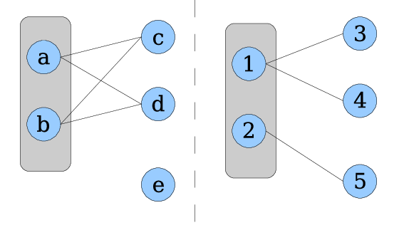
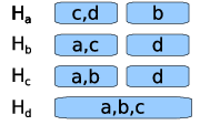
Roughly, elements of a umodule come from the same “school of thinking”: if one element of a umodule differentiates, resp. mixes together, some exterior elements, so does every element of the umodule (Fig. 1). A umodule $U$ is trivial if $|U|\leq 1$ or if $|U|\geq|X|-1$ . The family of umodules of $H$ is denoted by $\mathcal{U}_{H}$ , and $\mathcal{U}$ when no confusion occurs. $H$ is umodular prime if all umodules of $H$ are trivial. The following proposition links umodules to the $1$ -intersecting families framework as defined in [18]. The subsequent one tells how far umodules may generalise modules.

Proposition 2

For any two umodules $U,U^{\prime}$ of a homogeneous relation $H$ , if $U\cap U^{\prime}\neq\emptyset$ then $U\cup U^{\prime}$ is also a umodule of $H$ .

Proposition 3

If $H$ is a standard homogeneous relation (see Definition 2), then any module of $H$ is a umodule of $H$ . If $H$ is an arbitrary homogeneous relation over a finite set $X$ , then any module $M$ of $H$ is such that $X\setminus M$ is a umodule of $H$ .

In case of graphs, a natural question arises [10]: for which graphs the notions of module and umodule coincide? The following result, which can also be seen as a relaxed converse of Proposition 3, solves this problem. As with modules, let the umodules of a graph refer to those of its standard homogeneous relation. Notice here in a graph that the complementary of a umodule also is a umodule. A threshold graph is one that can be constructed from the single vertex by repeated additions of a single isolated or dominating vertex.

Proposition 4

$G$ is a threshold graph if and only if in all induced subgraph of $G$ , every umodule is either a module or the complementary of a module (or both).

Threshold graphs are known to be one of the smallest graph classes (see e.g. [2]). Therefore for most graphs umodules and modules differ, and Section 6 is devoted to the umodular graph decomposition. However, before deepening decomposition issues, let us first display umodule tractability.

3 Algorithmic Tractability for the general case

As far as we are aware, there is no evidence of a decomposition scheme for arbitrary umodules. The first valuable objects to compute thus seem to be the maximal umodules with respect to some cut. Using this, we also provide a polynomial time algorithm computing the strong umodules (see definition afterwards).

3.1 Maximal Umodules with respect to a cut

Partitions will be ordered with respect to the usual partition lattice: $\mathcal{P}=\{P_{1},\dots,P_{p}\}$ is coarser than $\mathcal{Q}=\{Q_{1},\dots,Q_{q}\}$ , and $\mathcal{Q}$ is thinner than $\mathcal{P}$ , if every part $Q_{i}$ is contained in some $P_{j}$ . It is noted $\mathcal{Q}\leq\mathcal{P}$ and $\mathcal{Q}<\mathcal{P}$ if the partitions are different. Let $S$ be a subset of $X$ . As the umodule family $\mathcal{U}$ is closed under union of intersecting members (Proposition 2), the inclusionwise maximal umodules included in either $S$ or $X\setminus S$ form a partition of $X$ , denoted by $MU(S)=MU(X\setminus S)$ . In other words, this is the coarsest partition of $X$ into umodules of $H$ , which is thinner than $\{S,X\setminus S\}$ . Roughly, it gives an indication on how the umodules are structured with respect to $S$ : a umodule either is included in a umodule of $MU(S)$ , or properly intersects $S$ , or properly intersects $X\setminus S$ , or trivial.

Definition 4

Let $H$ be a homogeneous relation over $X$ . Let $C\subseteq X$ . The relation $R_{C}$ on $C$ is defined as:

$\forall x,y\in C,R_{C}(x,y)\ if\ \forall a,b\in(X\setminus C)\ \ H(x|ab)\Longleftrightarrow H(y|ab).$

This clearly is an equivalence relation on $C$ . Furthermore, $C$ is a umodule if and only if $R_{C}$ only has one equivalence class. Let us define a refinement operation, the main algorithmic tool for constructing $MU(S)$ .

Definition 5

Let $\mathcal{P}$ be a partition of $X$ and $C$ a part of $\mathcal{P}$ . Let $C_{1},\ldots,C_{k}$ be the equivalence classes of $R_{C}$ . $Refine(\mathcal{P},C)$ is the partition obtained from $\mathcal{P}$ , by replacing part $C$ by the parts $C_{1},\ldots,C_{k}$ . A partition $\mathcal{P}$ is refinable by $C$ if $Refine(\mathcal{P},C)\neq\mathcal{P}$ . $\mathcal{P}$ is unrefinable if for every part $C$ of $\mathcal{P}$ , we have $\mathcal{P}=Refine(\mathcal{P},C)$ .

Lemma 1

Let $H$ be a homogeneous relation over $X$ , $U$ a umodule of $H$ , and $\mathcal{P}$ a partition of $X$ . If $U$ is included in a part of $\mathcal{P}$ , then for any part $C$ of $\mathcal{P}$ , $U$ is included in a part of $Refine(\mathcal{P},C)$ . Moreover, a part $C$ of $\mathcal{P}$ is a umodule if and only if $\mathcal{P}$ is not refinable by $C$ .

\mathcal{P}\leftarrow\{S,X\setminus S\}

while there exists an unmarked part $C$ in $\mathcal{P}$ do if $\mathcal{P}=Refine(\mathcal{P},C)$ then mark

C

else

\mathcal{P}\leftarrow Refine(\mathcal{P},C)

Algorithm 1 Refinement algorithm computing

MU(S)

given homogeneous relation

H

over

X

and

S\subseteq X

Correctness of Algorithm 1 follows from Lemma 1 and the invariant: There is no umodule partition $\mathcal{Q}$ such that $\mathcal{P}<\mathcal{Q}<\{S,X\setminus S\}$ . So, starting from $\{S,X\setminus S\}$ the algorithm constructs a strictly decreasing chain of partitions of $X$ ending at $MU(S)$ . Let us see how to implement it efficiently.

Lemma 2

It is possible to compute $Refine(\mathcal{P},C)$ in $O(|X|^{2})$ time.

We first show how to test for $R_{C}(x,y)$ . Compute, for every element $x$ of $C$ , a partition $\mathcal{H}(x,C)=\{P_{x}^{1},\ldots,P_{x}^{k(x)}\}$ of $X\setminus C$ . It is the restriction of $H_{x}$ to $X\setminus C$ , i.e $P_{x}^{i}=H_{x}^{i}\setminus C$ . It is easy to build in $O(|X|)$ time for each element of $C$ . Then we have $R_{C}(x,y)$ if and only if $H(x,C)$ is exactly the same partition than $H(y,C)$ . It can be tested in $O(|X|)$ time, but performing this for each couple of elements of $C$ would lead to an $O(|X|^{3})$ time implementation of $Refine(\mathcal{P},C)$ . Let us instead consider $\mathcal{H}(x,C)$ as a $b$ bit vectors (with $b=|X\setminus C|=O(|X|)$ ). Looking for duplicates among these vectors can be performed easily, by bucket sorting them on their first bit, then the second, and so on. A scan of all vectors (i.e. of all elements of $C$ ) compute the pairwise equal vectors, i.e the $R_{C}$ equivalent elements of $C$ . It is then easy to split $C$ and to update $\mathcal{P}$ , in $O(|X|^{2})$ time. $\Box$

The lemma above leads to an $O(|X|^{3})$ time implementation of Algorithm 1. However,

Theorem 1

For every $S\subseteq X$ , $MU(S)$ , the coarsest umodule partition thinner than $\{S,X-S\}$ can be computed in $O(|X|^{2}\log|X|)$ time.

Using the well-known Hopcroft’s partition refinement rule it is possible to improve the above algorithm. The idea is to avoid at each step to consider the biggest part, see [27]. Thus, to compute $MU(S)$ assuming that $|S|\leq|X-S|$ , we first partition $X-A$ using the ”neighbourhoods lists” of all $a\in A$ . If we assume a data structure which links each edge $ay$ to its opposite edge $ya$ . We can associate in the meantime to each element $a\in A$ a bitvector representing how $X-A$ sees $a$ . These $|A|$ bitvectors of size $|X-A|$ can be sorted in $O(|X|.|X-A|)\in O(|X|^{2})$ . Using Hopcroft’s rule, a vertex $a$ can only be explored at most $O(\log|X|)$ time, which yields the announced complexity. $\Box$

3.2 Strong Umodules: Maximal Umodules Computation and Primality Test

A umodule is strong if it overlap no other umodules, where two subsets overlap if none of the intersection and differences are empty. As two strong umodules are either disjoint, or one contains another, they can be ordered by inclusion into a tree (see e.g. laminar families in [28]).

Theorem 2

There exists an $O(|X|^{4}\log|X|)$ algorithm to compute the inclusion tree of strong umodules.

Consider a non-trivial strong umodule $M$ . For each pairwise distinct $x,y\notin M$ (at least two of them exists since $M$ is not trivial), $M$ is contained in exactly one set of $MU(\{x,y\})$ . The intersection of all these sets is exactly $M$ . Indeed if it where $M^{\prime}$ such that $M\subsetneq M^{\prime}$ then there would exist $x\in M^{\prime}\setminus M$ . For $y\notin M$ , $MU(\{x,y\})$ contains a umodule $M^{\prime\prime}$ smaller than $M^{\prime}$ but containing $M$ , a contradiction. Then the algorithm is as follow. For every pair $\{x,y\}$ compute $MU(\{x,y\})$ in $O(|X|^{2}\log|X|)$ time (Theorem 1). That gives a family of at most $|X|^{3}$ umodules. Add the trivial modules to the family. Greedily compute the intersection of overlapping umodules of the family. It is possible in $O(|X|^{4}\log|X|)$ time: for each triple $(a,b,c)$ look for the umodules containing exactly two of them, they overlap. Then we have all strong umodules. We finally just have to order them into a tree. $\Box$

This answers both maximal umodule computation and primality test since a non-trivial umodule exists if and only if a non-trivial strong umodule exists.

4 Two Decomposition Scenarios

Of course, the number of umodules may be as large as $2^{|X|}$ . But we shall now focus on certain umodule families having a compact (polynomial-size) representation. Umodules of local congruence 2 relations, on the first hand, and self-complemented umodules families, on the second hand, have such properties. They can be stored in $O(|X|^{2})$ and $O(|X|)$ space, respectively.

4.1 Local Congruence and Crossing Families

Definition 6 (Local congruence)

Let $H$ be a homogeneous relation on $X$ . For $x\in X$ , the congruence of $x$ is the maximal number of elements that $x$ pairwise distinguishes. In other words, it is the number of equivalence classes of $H_{x}$ . The local congruence of $H$ is the maximum congruence of the elements of $X$ .

Remark 1

The standard homogeneous relation of an undirected graph or a tournament has local congruence 2. This value is 3 for an antisymmetric directed graph or a directed acyclic graph. The value is 4 for digraphs.

When the local congruence of $H$ is $2$ , so-call LC2 condition for short, we obtain the following structural property on its umodule family.

Definition 7 (Crossing family)

$\mathcal{F}\subseteq 2^{X}$ is a crossing family if, for any $A,B\in\mathcal{F}$ , that $A\cap B\neq\emptyset$ and $A\cup B\neq X$ implies $A \cap B\in\mathcal{F}$ and $A \cup B\in\mathcal{F}$ (see e.g. [28] for further details).

Crossing families commonly arise as the minimisers of a submodular function. For instance, the minimum $s,t-$ cuts of a network form a crossing family. Gabow proved that a crossing family admits a compact representation in $O(|X|^{2})$ space using a tree representation [16].

Proposition 5

The umodules of a homogeneous relation with local congruence $2$ form a crossing family, and can thus be stored in $O(|X|^{2})$ space.

4.2 Self-complementarity and Bipartitive Families

A consequence of previous proposition is that standard homogeneous relations of graphs and tournaments have crossing umodules families. But they have stronger properties, which we will use to show a linear-space structure coding the umodule family.

Definition 8 (Four elements condition)

$H$ fulfils the four elements condition if

\displaystyle\forall~m,m^{\prime},x,x^{\prime}\in X,~~\left\{\begin{array}[]{l}H(m|xx^{\prime})\wedge H(m^{\prime}|xx^{\prime})\wedge H(x|mm^{\prime})\Rightarrow H(x^{\prime}|mm^{\prime})\\ \neg H(m|xx^{\prime})\wedge\neg H(m^{\prime}|xx^{\prime})\wedge\neg H(x|mm^{\prime})\Rightarrow\neg H(x^{\prime}|mm^{\prime})\end{array}\right..

Proposition 6

Standard homogeneous relations of undirected graphs and tournaments satisfy the four elements condition.

This is a light regularity condition, allowing to avoid examples similar to that of Fig. 1(b). Surprisingly enough, it suffices to make the umodule family behave in a very tractable manner (Proposition 7 and Corollary 1 below).

Definition 9 (Self-complementary condition)

A family $\mathcal{F}$ of subsets of $X$ is self-complemented if for every subset $A$ , $A\in\mathcal{F}$ implies $X\setminus A\in\mathcal{F}$ .

Proposition 7

If a homogeneous relation $H$ fulfils the four elements condition then the family $\mathcal{U}$ of umodules of $H$ is self-complemented.

The four elements condition is quite convenient since it allows to shrink a umodule, hence apply the divide and conquer paradigm to solve optimisation problems. However, as far as umodules are concerned, the self-complementary relaxation is sufficient to describe a tree-decomposition theorem as can be seen in the following section. Finally, notice that the converse of Proposition 7 does not necessarily hold. The characterisation of relations having a self-complemented umodule family by a local axiom, such as the four elements condition, actually appears to be more difficult.

4.2.1 Tree Decomposition Theorem

The following results on bipartitions can be found in [11] under the name of “decomposition frame with the intersection and transitivity properties”, in [24] under the name of “bipartitive families” (the formalism used in this paper), and in [21] under the name of “unrooted set families”.

We call $\{X_{i}^{1},X_{i}^{2}\}$ a bipartition of $X$ if $X_{i}^{1}\cup X_{i}^{2}=X$ and $X_{i}^{1}\cap X_{i}^{2}=\emptyset$ . Two bipartitions $\{X_{i}^{1},X_{i}^{2}\}$ and $\{X_{j}^{1},X_{j}^{2}\}$ overlap if for all $a,b=1,2$ the four intersections $X_{i}^{a}\cap X_{j}^{b}$ are not empty. A bipartition is trivial if one of the two parts is of size $1$ . Let $\mathcal{B}=\{\{X_{i}^{1},X_{i}^{2}\}_{i\in 1,\ldots,k}\}$ be a family of $k$ bipartitions of $X$ . The strong bipartitions of $\mathcal{B}$ are those that do not overlap any other bipartition of $\mathcal{B}$ . For instance, the trivial bipartitions of $\mathcal{B}$ are strong bipartitions of $\mathcal{B}$ .

Proposition 8

If $\mathcal{B}$ contains all trivial bipartitions of $X$ , then there exists a unique tree $T(\mathcal{B})$

•

with $|X|$ leaves, each leaf being labelled by an element of $X$ .
•

such that each edge $e$ of $T(\mathcal{B})$ correspond to a strong bipartition of $\mathcal{B}$ : the leaf labels of the two connected components of $T-e$ are exactly the two parts of a strong bipartition, and the converse also holds.

Let $N$ be a node of $T(\mathcal{B})$ of degree $k$ . The labels of the leaves of the connected components of $T-N$ form a partition $X_{1},\ldots,X_{k}$ of $X$ . For $I\subseteq\{1,\ldots,k\}$ with $1<|I|<k$ , the bipartition $B(I)$ is $\{\cup_{i\in I}X_{i},X\setminus\cup_{i\in I}X_{i}\}$ .

Definition 10 (Bipartitive Family)

A family of bipartitions is a bipartitive family if it contains all the trivial bipartitions and if, for two overlapping bipartitions $\{X_{i}^{1},X_{i}^{2}\}$ and $\{X_{j}^{1},X_{j}^{2}\}$ , the four bipartitions $\{X_{i}^{a}\cup X_{j}^{b},X\setminus(X_{i}^{a}\cup X_{j}^{b})\}$ (for all $a,b=1,2$ ) belong to $\mathcal{B}$ .

Theorem 3

[24] If $\mathcal{B}$ is a bipartitive family, the nodes of $T(\mathcal{B})$ can be labelled complete, circular or prime, and the children of the circular nodes can be ordered in such a way that:

•

If $N$ is a complete node, for any $I\subseteq\{1,\ldots,k\}$ such that $1<|I|<k$ , $B(I)\in\mathcal{B}$ .
•

If $N$ is a circular node, for any interval $I=[a,\ldots,b]$ of $\{1,\ldots,k\}$ such that $1<|b-a|<k$ , $B(I)\in\mathcal{B}$ .
•

If $N$ is a prime node, for any element $I=\{a\}$ of $\{1,\ldots,k\}$ $B(I)\in\mathcal{B}$ .
•

There are no more bipartitions in $\mathcal{B}$ than the ones described above.

For a bipartitive family $\mathcal{B}$ , the labelled tree $T(\mathcal{B})$ is an $O(|X|)$ -sized representation of $\mathcal{B}$ , while the family can have up to $2^{|X|-1}-1$ bipartitions of $|X|$ elements each. This allows to efficiently perform algorithmic operations on $\mathcal{B}$ . Notice that any self-complemented subset family can be seen as a family of bipartitions.

Proposition 9

The members of a self-complemented umodule family form a bipartitive family.

Corollary 1 (Umodular Decomposition Theorem)

There is a unique $O(|X|)$ -sized tree that gives a description of all possible umodules of a homogeneous relation $H$ fulfilling the self-complementary condition. This tree is henceforth called umodular decomposition tree. Notice that it is an unrooted tree, unlike the modular decomposition tree.

4.2.2 Tree Decomposition Algorithm

Let $H$ be a self-complemented homogeneous relation, $T(H)$ its umodular decomposition tree, and $U$ a nontrivial strong umodule (if any). Let us examine some consequences of Theorem 3. Notice that two umodules overlap if and only if they are incident to the same node of $T(H)$ . As $H$ is self-complemented the union of two overlapping umodules is a umodule (Proposition 2) but also their intersection. The strong umodule $U$ is an edge in $T(H)$ incident with two nodes $A$ and $B$ .

•

If one of them, say $A$ , is labelled prime then for any $x,y\notin U$ such that the least common ancestor of them in $T(H)$ is $A$ , then $U\in MU(\{x,y\})$ .
•

If one of them, say $A$ , is labelled circular then for any $x$ belonging to the subtree rooted in the successor of $U$ in the ordered circular list of $A$ , and for any $y$ belonging to the subtree rooted in the predecessor of $U$ , then $U\in MU(\{x,y\})$ .
•

If one of them, say $A$ , is labelled complete then the intersection, for all $x,y\notin U$ whose least common ancestor is $A$ , the intersection of all parts of $MU(\{x,y\})$ containing $U$ is exactly $U$ .

Theorem 2 then can be used to compute the strong umodule inclusion tree. After this, typing the nodes and ordering their sons according to the above definition is straightforward. Hence,

Theorem 4

There exists an $O(|X|^{4}\log(|X|))$ algorithm to compute the unique decomposition tree for a self complemented umodule family.

5 Seidel-switching Theorem, a potent Tractability

Standard homogeneous relations of graphs and tournaments are of local congruence 2, and their umodule families are self-complemented. Firstly this means we can either decompose those families using the crossing families decomposition or using the bipartitive decomposition. Moreover, relations that satisfy both the self-complementary and LC2 properties seem to own stronger potential. In particular, let us show a nice local transformation from the umodules of such a relation to the modules of another relation. This operation was first introduced in J. Seidel in [29] on undirected graphs. It was later studied by several authors interested in some computational aspects [9, 22] and structural properties [19, 20] and recently in [25]. The operation is referred to as Seidel switch in [20], and we will adopt this terminology. We generalise it to homogeneous relations but take a restricted case of switch, with the slight difference that we remove from the transformation an element (see Fig. 2(a)). For convenience, if $H$ is a homogeneous relation on $X$ and $s\in X$ , we also refer to the equivalence classes of $H_{s}$ as $H_{s}^{1},\dots,H_{s}^{k}$ .

Definition 11 (Seidel switch)

Let $H$ be a homogeneous relation of local congruence $2$ on $X$ , and $s$ an element of $X$ . The Seidel switch at $s$ transforms $H$ into the homogeneous relation $H(s)$ on $X\setminus\{s\}$ defined as follows.

\forall x\in X\setminus\{s\},H(s)^{1}_{x}=(H_{x}^{1}\Delta H_{s}^{j})\setminus\{s\}\ and\ H(s)^{2}_{x}=(H_{x}^{2}\Delta H_{s}^{j})\setminus\{s\}

with $j$ such that $x\notin H_{s}^{j}$ . where $A\Delta B$ denotes the symmetric difference of $A$ and $B$ .

Theorem 5 (Seidel-switching Theorem)

Let $H$ be a homogeneous relation of local congruence $2$ on $X$ such that $\mathcal{U}_{H}$ is self-complemented. Let $s$ be a member of $X$ , and $U\subseteq X$ a subset containing $s$ . Then, $U$ is a umodule of $H$ if and only if $M=X\setminus U$ is a module of the Seidel switch $H(s)$ .

Corollary 2

The umodular decomposition tree of a self-complemented homogeneous relation of local congruence $2$ on $X$ can be computed in $O(|X|^{2})$ time.

Using a Seidel switch on any element will result in a relation having the so-called modular quotient property [3]: every module of the relation also is a umodule. Then, the $O(|X|^{2})$ -time modular decomposition algorithm for modular quotient relations depicted in [3]. As two complemented strong umodules $M,X\setminus M$ of $H$ , for $s\notin M$ , correspond to a strong module $M$ of $H(s)$ , then the strong umodules of $H$ can be found trivially from the strong modules of $H(s)$ . Typing and ordering their sons is then easy. $\Box$

Notice that the modular decomposition tree of $H$ can be trivial, while the one of its Seidel switch at $s$ may be not. Besides, there is no real need to type and order the sons of a node, as so-called linear nodes of the modular decomposition tree give circular nodes of the umodular decomposition tree with the same ordering of their sons, complete nodes of $H(s)$ give complete nodes of $H$ and prime nodes of $H(s)$ give prime nodes of $H$ . The correspondence is straightforward but modular decomposition of homogeneous relations will not be discussed here, the reader should refer to [3].

6 Umodular Decomposition of Graphs and Tournaments

Let us now apply umodular decomposition to two well-known combinatorial objects: undirected graphs and tournaments. In this section we always implicitly refer to their standard homogeneous relations, for instance “the umodules of the graph $G$ ” stands for “the umodules of the standard homogeneous relation $H(G)$ of the graph $G$ ” and so on. And “graph” stands for “undirected graph”. As we have seen, graphs and tournaments fulfil the four elements conditions, are of local congruence two, and their umodule family is self-complemented.

6.1 Bijoin decomposition

Let us call bijoin a umodule of a graph or of a tournament. From definition, one can see what bijoins are (Fig.2(b)). In a graph, $B$ is a bijoin if $X\setminus B$ can be partitioned in two sets $C$ and $D$ such that for each $x\in B$ , either $N(x)\cap C=\emptyset$ and $D\subseteq N(x)$ , or $N(x)\cap D=\emptyset$ and $C\subseteq N(x)$ . For a tournament, same definition with $C\subseteq N^{+}(x)$ and $D\subseteq N^{-}(x)$ , or $D\subseteq N^{+}(x)$ and $C\subseteq N^{-}(x)$ .

Bijoins of graphs where studied in [25] as a new graph decomposition, generalising modular decomposition. The Seidel switch was used to derive most of the properties claimed, especially a decomposition tree (with no circular nodes), a linear-time decomposition algorithm, a characterisation of the two kinds of complete nodes, and characterisation of totally decomposable graphs (see below).

Bijoins of tournaments form a new decomposition. The first important property is:

Proposition 10

The umodular (bijoin) decomposition tree computation time of a tournament is $O(|X|^{2})$ .

The tree exists thanks to Corollary 1, since the bijoins form a self-complemented $LC2$ family. The computation algorithm is from Corollary 2.

Proposition 11

The umodular (bijoin) decomposition tree of a tournament has no complete node. And there exists a circular ordering of the vertices of the tournament such that every umodule of the tournament is a factor (interval) of this circular ordering.

The first assumption can be checked by reader: it is impossible to build tournaments with more than four elements such that every vertex subset is a bijoin. The second is a consequence of the first, and of definitions in Theorem 3. As a consequence, there are $O(|X|^{2})$ bijoins in a tournament (the exponential growth of a bipartitive family comes from complete nodes).

6.2 Total Decomposability

Given a graph decomposition scheme, is often worth to consider the totally decomposable graphs with respect to that scheme, namely the graphs in which every ”large enough” subgraph admits a non trivial decomposition. In general this leads to the definition of very interesting class of graphs, such as cographs with modular decomposition or distance hereditary graphs with split decomposition. Let us now see how the graphs and tournaments totally decomposable with respect to bijoin decomposition behave.

Theorem 6

[25] The totally decomposable graph with respect to bijoin decomposition are the ( $C_{5}$ ,bull,gem,co-gem)-free graphs, and also exactly the graphs that can be obtained from a single vertex by a sequence of (twin,antitwin)-extensions.

Definition 12

A diamond is one of the induced subgraph described in Figure 3. A tournament $T$ is locally transitive if for each vertex $x\in V(T)$ , $T_{[N^{+}{(x)}]}$ and $T_{[N^{-}{(x)}]}$ are transitive tournaments. Two vertices $x$ and $y$ of a tournaments are twins if $N^{+}(x)\setminus\{y\}=N^{+}(y)\setminus\{x\}$ and antitwins if $N^{+}(x)\setminus\{y\}=N^{-}(y)\setminus\{x\}$ . An extension of a vertex $x$ of $T$ by a twin (resp. antitwin) $y$ consists in adding a new vertex $y$ to $T$ and making $y$ twin (resp. antitwin) of $x$ .

Theorem 7

Let $T$ be a tournament. The following propositions are equivalent:

1.

$T$ is diamond-free (no induced subgraph is a diamond)
2.

$T$ is locally transitive
3.

$T$ is totally decomposable with respect to bijoin decomposition
4.

$T$ can be obtained from a single vertex by a sequence of (twin,antitwin)-extensions.

As the in- and out-diamond are prime with respect to umodular decomposition, and total decomposability is an hereditary property, Point 3 implies Point 1. Let us sketch the proof that Point 2 implies Point 3. If $T$ is locally transitive then a Seidel switch of $T$ at any vertex $s$ produces a transitive tournament $T(s)$ . Every subgraph of a transitive tournament contains a module. So, according to Theorem 5, every subgraph of $T$ contains a umodule: $T$ is totally decomposable. Besides, the equivalence between Point 3 and Point 4 comes from the fact that, if $T$ is totally decomposable, then it contains a umodule of two vertices. Such umodules are made either with two twins or with two antitwins. Equivalence between 1 and 2 can be found in [1]. $\Box$

Figure 3: Forbidden subgraphs of a totally decomposable tournament with respect to umodular decomposition: the in-diamond(left) and the out-diamond(right).

It is not hard to check that, as the umodular decomposition tree of a totally decomposable tournament may have no prime node, and since two circular node may not be adjacent, then the umodular decomposition tree of a totally decomposable tournament has only a single circular node. The ordering of the vertices along this node is known as circular ordering. This ordering is such that, for each vertex $x$ , the vertices of $N^{+}(x)$ follow consecutively; and so do vertices from $N^{-}(x)$ . This, combined to the above theorem, could be seen as a sketched proof of the characterisation of round tournaments by local transitivity (see e.g. [1] for further information).

In the extended version [6], we present an $O(n^{2})$ recognition algorithm, making an intensive use of this ordering property, and computing this ordering. It allows us to solve the isomorphism problem for the class of such tournament in $O(n^{2})$ time, like in [8]. We also propose the first linear-time algorithm for the feedback vertex set problems (NP-complete for tournaments). The basic idea is to find a vertex of highest outgoing degree, and output the tournament composed of this vertex and its outgoing neighbourhood.

7 Extensions and further developments

We have presented the umodules and homogeneous relations focusing on graph theory field. But umodules may be found in many other objects. For instance, if we take a commutative ring and define

$H_{\times}(x|yz)\ \iff\ xy=xz,$

then the principal ideals of the ring are umodules. In this paper we study umodular decomposition applied to graphs, when the local congruence is 2, the next challenge is now to understand umodular decomposition of directed graphs or directed acyclic graphs, starting with the self-complemented case first.

Our computation of strong umodules is polynomial, but its asymptotic complexity of $O(|X|^{4}.\log(|X|))$ can surely be reduced, especially when applied to particular combinatorial objects.

We have noticed here the great importance of the Seidel switch operation, and following the notion of vertex minor as defined in [26], let us called $H$ a Seidel minor of a graph $G$ , if $H$ can be obtained from $G$ by the two following operations:

•

delete a vertex,
•

choose a vertex and do a Seidel switch on this vertex

It could be of interest to study such Seidel minors.

References

[1] J. Bang-Jensen and G. Gutin. Digraphs: Theory, Algorithms and Applications. Springer Monographs in Mathematics. Springer-Verlag, 2001.
[2] A. Brandstadt, V.B. Le, and J.P. Spinrad. Graph Classes: A Survey. SIAM Monographs on Discrete Mathematics and Applications. Society for Industrial and Applied Mathematics, 1999.
[3] B.-M. Bui-Xuan, M. Habib, V. Limouzy, and F. de Montgolfier. Algorithmic aspects of a novel modular decomposition theory. Technical report, http://hal.archives-ouvertes.fr/hal-00111235, 2006. Submitted.
[4] B.-M. Bui Xuan, M. Habib, V. Limouzy, and F. de Montgolfier. Homogeneity vs. adjacency: generalising some graph decomposition algorithms. In 32nd International Workshop on Graph-Theoretic Concepts in Computer Science (WG), volume 4271 of LNCS, June 2006.
[5] B.-M. Bui-Xuan, M. Habib, V. Limouzy, and F. de Montgolfier. On modular decomposition concepts: the case for homogeneous relations. Electronic Notes in Discrete Mathematics, 27, 2006.
[6] B.-M. Bui-Xuan, M. Habib, V. Limouzy, and F. de Montgolfier. A new tractable decomposition. Technical report, http://hal-lirmm.ccsd.cnrs.fr/lirmm-00157502, 2007.
[7] M. Chein, M. Habib, and M. C. Maurer. Partitive hypergraphs. Discrete Mathematics, 37(1):35–50, 1981.
[8] E. Clarou. Une hiérarchie de forçage pour les tournois indécomposables. PhD thesis, Université Claude Bernard Lyon I, 1996.
[9] C. J. Colbourn and D. G. Corneil. On deciding switching equivalence of graphs. Discrete Applied Mathematics, 2(3):181–184, 1980.
[10] D. G. Corneil. Private communication. Dagstuhl, 2007.
[11] W. H. Cunningham. A combinatorial decomposition theory. PhD thesis, University of Waterloo, Waterloo, Ontario, Canada, 1973.
[12] A. Ehrenfeucht, T. Harju, and G. Rozenberg. The Theory of 2-Structures- A Framework for Decomposition and Transformation of Graphs. World Scientific, 1999.
[13] A. Ehrenfeucht and G. Rozenberg. Theory of 2-structures. Theoretical Computer Science, 3(70):277–342, 1990.
[14] M. G. Everett and S. P. Borgatti. Role colouring a graph. Mathematical Social Sciences, 21:183–188, 1991.
[15] J. Fiala and D. Paulusma. The computational complexity of the role assignment problem. In 30th International Colloquium on Automata, Languages and Programming (ICALP), pages 817–828, 2003.
[16] H. N. Gabow. A representation for crossing set families with applications to submodular flow problems. In Proceedings of the Fourth Annual ACM-SIAM Symposium on Discrete Algorithms (SODA), pages 202–211. ACM/SIAM, 1993.
[17] T. Gallai. Transitiv orientierbare Graphen. Acta Math. Acad. Sci. Hungar., 18:25–66, 1967.
[18] M. Habib and M. C. Maurer. 1-intersecting families. Discrete Mathematics, 53:91–101, 1985.
[19] R. B. Hayward. Recognizing 3-structure: A switching approach. Journal of Combinatorial Theory, Serie B, 66(2):247–262, 1996.
[20] A. Hertz. On perfect switching classes. Discrete Applied Mathematics, 94(1-3):3–7, 1999.
[21] W.-L. Hsu and R. M. McConnell. PC-trees and circular-ones arrangements. Theoretical Computer Science, 296:99–116, 2003.
[22] J. Kratochvíl, J. Nešetřil, and O. Zýka. On the computational complexity of Seidel’s switching. In Fourth Czechoslovakian Symposium on Combinatorics, Graphs and Complexity (Prachatice, 1990), volume 51 of Ann. Discrete Math., pages 161–166. North-Holland, Amsterdam, 1992.
[23] R. H. Möhring and F. J. Radermacher. Substitution decomposition for discrete structures and connections with combinatorial optimization. Annals of Discrete Mathematics, 19:257–356, 1984.
[24] F. de Montgolfier. Décomposition modulaire des graphes. Théorie, extensions et algorithmes. PhD thesis, Université Montpellier II, 2003.
[25] F. de Montgolfier and M. Rao. The bi-join decomposition. In ICGT ’05, 7th International Colloquium on Graph Theory, 2005.
[26] S.-I. Oum. Rank-width and vertex-minors. Journal of Combinatorial Theory, Series B, 95(1):79–100, 2005.
[27] R. Paige and R. E. Tarjan. Three partition refinement algorithms. SIAM Journal on Computing, 16(6):973–989, 1987.
[28] A. Schrijver. Combinatorial Optimization - Polyhedra and Efficiency. Springer-Verlag, 2003.
[29] J. J. Seidel. A survey of two-graphs. In Colloquio Internazionale sulle Teorie Combinatorie (Rome, 1973), Tomo I, pages 481–511. Atti dei Convegni Lincei, No. 17. Accad. Naz. Lincei, Rome, 1976.
[30] D. R. White and K. P. Reitz. Graph and semigroup homomorphisms on networks of relations. Social Networks, 5:193–234, 1983.

Unifying two Graph Decompositions with Modular Decomposition0