跳到论文正文
W Papers独立论文阅读器 arXiv:cs/0604033 论文正文 计算阅读时间 · 0%
引用这篇论文根据当前论文元数据生成,正式投稿前建议核对。


License: Assumed arXiv.org perpetual non-exclusive license
arXiv:cs/0604033v1 [cs.IT] 08 Apr 2006

Statistical Properties of Eigen-Modes and Instantaneous Mutual Information in MIMO Time-Varying Rayleigh ChannelsThis paper was presented in part at the 40th Ann. Conf. Info. Sci. Sys., Princeton, NJ, 2006.The authors are with the Center for Wireless Communications and Signal Processing Research (CWCSPR), Department of Electrical and Computer Engineering, New Jersey Institute of Technology, Newark, NJ 07102 USA (e-mail:{sw27, ali.abdi}@njit.edu).

Shuangquan Wang, and Ali Abdi
Abstract

In this paper, we study two important metrics in multiple-input multiple-output (MIMO) time-varying Rayleigh flat fading channels. One is the eigen-mode, and the other is the instantaneous mutual information (IMI). Their second-order statistics, such as the correlation coefficient, level crossing rate (LCR), and average fade/outage duration, are investigated, assuming a general nonisotropic scattering environment. Exact closed-form expressions are derived and Monte Carlo simulations are provided to verify the accuracy of the analytical results. For the eigen-modes, we found they tend to be spatio-temporally uncorrelated in large MIMO systems. For the IMI, the results show that its correlation coefficient can be well approximated by the squared amplitude of the correlation coefficient of the channel, under certain conditions. Moreover, we also found the LCR of IMI is much more sensitive to the scattering environment than that of each eigen-mode.

Index Terms:
Eigen-Modes, Instantaneous Mutual Information, Autocorrelation Function, Correlation Coefficient, Level Crossing Rate, Average Fade/Outage Duration, and Multiple-Input Multiple-Output (MIMO).

I Introduction

The utilization of antenna arrays at the base station (BS) and the mobile station (MS) in a wireless communication system increases the capacity linearly with min⁡(NT,NR)\min(N_{\!T},N_{\!R}), under certain conditions, where NTN_{\!T} and NRN_{\!R} are numbers of transmit and receive antenna elements, respectively, provided that the environment is sufficiently rich in multi-path components [1, 2]. This is due to the fact that a multiple-input multiple-output (MIMO) channel can be decomposed to several parallel single-input single-output (SISO) channels, called eigen-channels or eigen-modes11 1 We use the two terms interchangeably in this paper., via singular value decomposition (SVD)[2, 3, 4, 5, 6, 7, 8, 9].

For a SISO channel, or any subchannel22 2 In this paper, each subchannel represents the radio link between each transmit/receive pair of antennas. of a MIMO system, there are numerous studies on key second-order statistics such as correlation, level crossing rate (LCR), and average fade duration (AFD)[10, 11, 12, 13, 14]. However, to the best of our knowledge, no such study on the eigen-channels of a MIMO system is reported in the literature, possibly due to the lack of knowledge regarding the joint probability density function (PDF) of eigen-channels.

Regarding another important quantity, the instantaneous mutual information (IMI), only some first-order statistics such as the mean, variance, outage probability and PDF are studied[15, 16, 17, 18, 9]. Clearly, those statistics do not show the dynamic temporal behavior, such as correlations, LCR and average outage durations (AOD) of the IMI in time-varying fading channels. It is known that IMI can be feedbacked to the rate scheduler in multi-user communication environments, to increase the system throughput[16], where only the perfect feedback is considered. However, it is hard to obtain perfect feedback in practice due to the time-varying nature of the channel, which makes the feedbacked IMI outdated. In this case, the temporal correlation of IMI can be used to analyze the scheduling performance with outdated IMI feedbacks. Furthermore, one can improve the rate scheduling algorithm by exploring the temporal correlation of IMI.

Several second-order statistics such as the correlation coefficient, LCR and AOD of IMI in single-input single-output (SISO) systems are reported in [19] and [20]. For MRC-like MIMO systems, they are investigated in [20]. However, there are a limited number of results for a general MIMO channel. In [21], some simulation results regarding the correlation coefficient, LCR and AOD are reported, without analytical derivations. In [22], lower and upper bounds, as well as some approximations for the correlation coefficient of IMI are derived, without exact results at high SNR. A large gap between the lower and upper bounds and large approximation errors are observed in [22, Figs. 2, 5].

In this paper, we extend the results of [20] to the general MIMO case, using the joint PDF of the eigenvalues[23]. Specifically, a number of second-order statistics such as the autocorrelation function (ACF), the correlation coefficient, LCR and AFD/AOD33 3 Note that AFD is used for eigen-channels, whereas AOD is used for MIMO IMI. of the eigen-channels and the IMI are studied in MIMO time-varying Rayleigh flat fading channels. We assume all the subchannels are spatially independent and identically distributed (i.i.d.), with the same temporal correlation coefficient, considering general nonisotropic scattering propagation environments. Closed-form expressions are derived, and Monte Carlo simulations are provided to verify the accuracy of our closed-form expressions. The simulation and analytical results show that the eigen-modes tend to be spatio-temporally uncorrelated in large MIMO systems, and the correlation coefficient of the IMI can be well approximated by the squared amplitude of the correlation coefficient of the channel if |NT−NR||N_{\!T}-N_{\!R}| is much larger than min⁡(NT,NR)\min\left(N_{\!T},N_{\!R}\right). In addition, we also observed that the LCR of IMI is much more sensitive to the scattering environment than that of each eigen-mode.

The rest of this paper is organized as follows. Section II introduces the channel model, as well as the angle-of-arrival (AoA) model. Eigen-channels of a MIMO system are discussed in Section III, where Subsection III-A is devoted to the derivation of the normalized ACF (NACF) and the correlation coefficient of eigen-channels of a MIMO system, whereas Subsection III-B focuses on the LCR and AFD of the eigen-channels. The MIMO IMI is investigated in Section IV, in which Subsection IV-A addresses the NACF and the correlation coefficient of the MIMO IMI as well as their low- and high-SNR approximations, whereas Subsection IV-B studies the LCR and AOD of the MIMO IMI using the well-known Gaussian approximation. Numerical results and discussions are presented in Section V, and concluding remarks are given in Section VI.

Notation: ⋅†\cdot^{{\dagger}} is reserved for matrix Hermitian, ⋅⋆\cdot^{\star} for complex conjugate, ȷ\jmath for −1\sqrt{-1}, 𝔼⁡[⋅]\mathbb{E}[\cdot] for mathematical expectation, 𝐈m\mathbf{I}_{m} for the m×mm\times m identity matrix, ∥⋅∥F\|\cdot\|_{F} for the Frobenius norm, ℜ⁡[⋅]\Re[\cdot] and ℑ⁡[⋅]\Im[\cdot] for the real and imaginary parts of a complex number, respectively, and f2​(x)f^{2}(x) for [f⁡(x)]2\left[f(x)\right]^{2}. Finally, t∈[m,n]t\!\!\in\!\![m,n] implies that tt, mm and nn are integers such that m≤t≤nm\leq t\leq n with m≤nm\leq n.

II Channel Model

In this paper, an NR×NTN_{\!R}\times N_{\!T} MIMO time-varying Rayleigh flat fading channel is considered. Similar to [15], we consider a piecewise constant approximation for the continuous-time MIMO fading channel matrix coefficient 𝐇⁡(t)\mathbf{H}(t), represented by {𝐇⁡(l​Ts)}l=1L\left\{\mathbf{H}(lT_{\!s})\right\}_{l=1}^{L}, where TsT_{\!s} is the symbol duration and LL is the number of samples. In the sequel, we drop TsT_{\!s} to simplify the notation. In the lthl^{\mathrm{th}} symbol duration, the matrix of the channel coefficients is given by

𝐇⁡(l)=[h1,1​(l)⋯h1,NT​(l)⋱hNR,1​(l)⋯hNR,NT​(l)],l∈[1,L].\mathbf{H}(l)=\begin{bmatrix}h_{1,1}(l)&\cdots&h_{1,N_{\!T}}(l)\\ \vdots&\ddots&\vdots\\ h_{N_{\!R},1}(l)&\cdots&h_{N_{\!R},N_{\!T}}(l)\\ \end{bmatrix},l\in[1,L]. (1)

We assume all the NT​NRN_{\!T}N_{\!R} subchannels {hnr,nt​(l),l∈[1,L]}(nr=1,nt=1)(NR,NT)\left\{h_{n_{r},n_{t}}(l),l\in[1,L]\right\}_{(n_{r}=1,n_{t}=1)}^{(N_{\!R},N_{\!T})} are i.i.d., with the same temporal correlation coefficient, i.e.,

𝔼⁡[hm​n​(l)​hp​q⋆​(l−i)]=δm,p​δn,q​ρh​(i),\mathbb{E}[h_{mn}(l)h_{pq}^{\star}(l-i)]=\delta_{m,p}\delta_{n,q}\rho_{h}(i), (2)

where the Kronecker delta δm,p\delta_{m,p} is 11 or 00 when m=pm=p or m≠pm\neq p, respectively, and ρh​(i)\rho_{h}(i) is defined and derived at the end of this section, eq. (4).

In flat Rayleigh fading channels, each hnr,nt​(l),l∈[1,L]h_{n_{r},n_{t}}(l),l\in[1,L], is a zero-mean complex Gaussian random process. In the lthl^{\mathrm{th}} interval, hnr,nt​(l)h_{n_{r},n_{t}}(l) can be represented as[13]

hnr,nt​(l)=hnr,ntI​(l)+ȷ​hnr,ntQ​(l),=αnr,nt​(l)​exp⁡[−ȷ​Φnr,nt​(l)],\begin{split}h_{n_{r},n_{t}}(l)&=h_{n_{r},n_{t}}^{I}(l)+\jmath h_{n_{r},n_{t}}^{Q}(l),\\ &=\alpha_{n_{r},n_{t}}(l)\exp[-\jmath\Phi_{n_{r},n_{t}}(l)],\end{split} (3)

where the zero-mean real Gaussian random processes hnr,ntI​(l)h_{n_{r},n_{t}}^{I}(l) and hnr,ntQ​(l)h_{n_{r},n_{t}}^{Q}(l) are the real and imaginary parts of hnr,nt​(l)h_{n_{r},n_{t}}(l), respectively. αnr,nt​(l)\alpha_{n_{r},n_{t}}(l) is the envelope of hnr,nt​(l)h_{n_{r},n_{t}}(l) and Φnr,nt​(l)\Phi_{n_{r},n_{t}}(l) is the phase of hnr,nt​(l)h_{n_{r},n_{t}}(l). For each ll, αnr,nt​(l)\alpha_{n_{r},n_{t}}(l) has a Rayleigh distribution and Φnr,nt​(l)\Phi_{n_{r},n_{t}}(l) is distributed uniformly over [−π,π)[-\pi,\pi). Without loss of generality, we assume each subchannel has unit power, i.e., 𝔼⁡[αnr,nt2​(l)]=1\mathbb{E}[\alpha^{2}_{n_{r},n_{t}}(l)]=1.

Using empirically-verified[13] multiple von Mises PDF’s[19, (4)] for the AoA at the receiver in nonisotropic scattering environments, shown as Fig. 1 of [19], the channel correlation coefficient of hnr,nt​(l)h_{n_{r},n_{t}}(l), ∀nr,nt\forall n_{r},n_{t}, is given by[19, (7)]

ρh​(i)=𝔼⁡[hnr,nt​(l)​hnr,nt⋆​(l−i)],=∑n=1NPn​I0​(κn2−4π2fD2i2Ts2+ȷ4πκnfDiTscosθn)I0​(κn),\begin{split}\rho_{h}(i)&=\mathbb{E}[h_{n_{r},n_{t}}(l)h_{n_{r},n_{t}}^{\star}(l-i)],\\ &=\!\sum_{n=1}^{N}\!P_{n}\!\frac{I_{0}\!\!\left(\!\!\sqrt{\kappa_{n}^{2}-4\pi^{2}f_{\!D}^{2}i^{2}T_{\!s}^{2}+\jmath 4\pi\kappa_{n}f_{\!D}iT_{\!s}\cos\theta_{n}}\right)}{I_{0}(\kappa_{n})},\end{split} (4)

where Ik​(z)=1π​∫0πez​cos⁡w​cos⁡(k​w)​d​wI_{k}(z)=\frac{1}{\pi}\int_{0}^{\pi}e^{z\cos w}\cos(kw)\text{d}w is the kthk^{\text{th}} order modified Bessel function of the first kind, θn\theta_{n} is the mean AoA of the nthn^{\text{th}} cluster of scatterers, κn\kappa_{n} controls the width of the nthn^{\text{th}} cluster of scatterers, PnP_{n} represents the contribution of the nthn^{\text{th}} cluster of scatterers such that ∑n=1KPn=1,0<Pn≤1\sum_{n=1}^{K}P_{n}=1,0<P_{n}\leq 1, KK is the number of clusters of scatterers, and fDf_{\!D} is the maximum Doppler frequency. When κn=0,∀n\kappa_{n}=0,\forall n, which corresponds to isotropic scattering, (4) reduces to ρh​(i)=I0​(ȷ​2​π​fD​i​Ts)=J0​(2​π​fD​i​Ts)\rho_{h}(i)=I_{0}(\jmath 2\pi f_{\!D}iT_{\!s})=J_{0}(2\pi f_{\!D}iT_{\!s}), which is the Clarke’s correlation model.

III Eigen-Channels in MIMO Systems

We set M=min⁡(NT,NR)M=\min\left(N_{\!T},N_{\!R}\right) and N=max⁡(NT,NR)N=\max\left(N_{\!T},N_{\!R}\right). Based on singular value decomposition (SVD)[2, 3, 4, 5, 6, 7, 8, 9], 𝐇⁡(l)\mathbf{H}(l) in (1) can be diagonalized in the following form

𝐇⁡(l)=𝐔⁡(l)​𝐒​(l)​𝐕†​(l),\mathbf{H}(l)=\mathbf{U}(l)\mathbf{S}(l)\mathbf{V}^{\dagger}(l), (5)

where 𝐕⁡(l)\mathbf{V}(l), whose dimension is NT×MN_{\!T}\times M, satisfies 𝐕†​(l)​𝐕​(l)=𝐈M\mathbf{V}^{\dagger}(l)\mathbf{V}(l)=\mathbf{I}_{M}, 𝐔⁡(l)\mathbf{U}(l), which is NR×MN_{\!R}\times M, satisfies 𝐔†​(l)​𝐔​(l)=𝐈M\mathbf{U}^{\dagger}(l)\mathbf{U}(l)=\mathbf{I}_{M}, and 𝐒⁡(l)\mathbf{S}(l) is a diagonal matrix, given by 𝐒⁡(l)=diag⁡[s1​(l),⋯,sM​(l)]\mathbf{S}(l)=\mathrm{diag}\left[s_{1}(l),\cdots,s_{M}(l)\right], in which sm​(l)s_{m}(l), m∈[1,M]m\in[1,M] is the mthm^{\mathrm{th}} non-zero singular value of 𝐇⁡(l)\mathbf{H}(l).

We define λm​(l)=sm2​(l)\lambda_{m}(l)=s_{m}^{2}(l), ∀m\forall m. Therefore λm​(l)\lambda_{m}(l) is the mthm^{\mathrm{th}} non-zero eigenvalue of 𝐇⁡(l)​𝐇†​(l)\mathbf{H}(l)\mathbf{H}^{\dagger}(l). We further consider {λm​(l)}m=1M\left\{\lambda_{m}(l)\right\}_{m=1}^{M} as unordered non-zero eigenvalues of 𝐇⁡(l)​𝐇†​(l)\mathbf{H}(l)\mathbf{H}^{\dagger}(l). Therefore, the MIMO channel 𝐇⁡(l)\mathbf{H}(l) is decomposed to MM identically distributed eigen-channels, {λm​(l),l∈[1,L]}m=1M\left\{\lambda_{m}(l),l\in[1,L]\right\}_{m=1}^{M}, by SVD, as shown in Fig. 1. For M=1M=1, there is only one eigen-channel, which corresponds to the maximal ratio transmitter (MRT) if NR=1N_{\!R}=1, or the maximal ratio combiner (MRC) if NT=1N_{\!T}=1. In each case, we have NN i.i.d complex Gaussian branches.

Since all the eigen-channels have identical statistics, we only study one of them and denote it as λ⁡(l),l∈[1,L]\lambda(l),l\in[1,L]. To simplify the notation, we use XX and YY to denote λ⁡(l)\lambda(l) and λ⁡(l−i)\lambda(l-i), respectively. The joint PDF of XX and YY is given in (6) of [23],

p⁡(x,y)\displaystyle p(x,y) =(x​y)ν2​e−x+y1−ϱi2​Iν​(2​ϱi​x​y1−ϱi2)M2​(1−ϱi2)​ϱiν∑k=0M−1k!​Lkν​(x)​Lkν​(y)(k+ν)!​ϱi2​k+(x​y)ν​e−(x+y)M2∑0≤k<lM−1{k!​l!(k+ν)!​(l+ν)!\displaystyle=\frac{(xy)^{\frac{\nu}{2}}e^{-\frac{x+y}{1-\varrho_{i}^{2}}}I_{\nu}\left(\frac{2\varrho_{i}\sqrt{xy}}{1-\varrho_{i}^{2}}\right)}{M^{2}(1-\varrho_{i}^{2})\varrho_{i}^{\nu}}\sum_{k=0}^{M-1}\frac{k!L_{k}^{\nu}(x)L_{k}^{\nu}(y)}{(k+\nu)!\varrho_{i}^{2k}}+\frac{(xy)^{\nu}e^{-(x+y)}}{M^{2}}\sum_{0\leq k<l}^{M-1}\bigg\{\frac{k!l!}{(k+\nu)!(l+\nu)!}
×{[Lkν(x)Llν(y)]2+[Llν(x)Lkν(y)]2−[ϱi2​(l−k)+ϱi2​(k−l)]Lkν(x)Llν(x)Lkν(y)Llν(y)}},\displaystyle\hskip 10.00002pt\times\left\{\left[L_{k}^{\nu}(x)L_{l}^{\nu}(y)\right]^{2}+\left[L_{l}^{\nu}(x)L_{k}^{\nu}(y)\right]^{2}-\left[\varrho_{i}^{2(l-k)}+\varrho_{i}^{2(k-l)}\right]L_{k}^{\nu}(x)L_{l}^{\nu}(x)L_{k}^{\nu}(y)L_{l}^{\nu}(y)\right\}\!\!\bigg\}, (6)

where Lnα​(x)=1n!​ex​x−α​dnd​xn​(e−x​xn+α)L_{n}^{\alpha}(x)=\frac{1}{n!}e^{x}x^{-\alpha}\frac{\mathrm{d}^{n}}{\mathrm{d}x^{n}}\left(e^{-x}x^{n+\alpha}\right) is the associated Laguerre polynomial of order nn[24, pp. 1061, 8.970.1], ν=N−M\nu=N-M, and ϱi=|ρh​(i)|\varrho_{i}=\left|\rho_{h}(i)\right|, where ρh​(i)\rho_{h}(i) is given in (4). The joint PDF in (6) is very general and includes many existing PDF’s as special cases[23].

  • •

    By integration over yy, (6) reduces to the marginal PDF

    p⁡(x)=1M​∑m=0M−1m!(m+ν)!​[Lmν​(x)]2​xν​e−x,p(x)=\frac{1}{M}\sum_{m=0}^{M-1}\frac{m!}{(m+\nu)!}\left[L_{m}^{\nu}(x)\right]^{2}x^{\nu}e^{-x}, (7)

    which is the same as the PDF presented in [2]. When M=1M=1, (7) further reduces to

    p⁡(x)=1(N−1)!​xN−1​e−x,p(x)=\frac{1}{(N-1)!}x^{N-1}e^{-x}, (8)

    which is the χ2\chi^{2} distribution with 2​N2N degrees of freedom[25, (2.32)], used for characterizing the PDF of outputs of MRT or MRC[26].

  • •

    With M=1M=1, (6) reduces to

    p⁡(x,y)=(x​y)N−12​exp⁡(−x+y1−ϱi2)​IN−1​(2​ϱi​x​y1−ϱi2)(N−1)!​(−ϱi2)​ϱiN−1,p(x,y)=\frac{(xy)^{\frac{N-1}{2}}\exp\left(\!-\frac{x+y}{1-\varrho_{i}^{2}}\!\right)I_{N-1}\!\left(\frac{2\varrho_{i}\sqrt{xy}}{1-\varrho_{i}^{2}}\right)}{(N-1)!\left(1\!-\!\varrho_{i}^{2}\right)\varrho_{i}^{N-1}}, (9)

    which is the joint PDF of outputs of MRT or MRC at the lthl^{\mathrm{th}} and (l−i)th(l-i)^{\mathrm{th}} symbol durations[27]. It includes (3.14) of [25] as a special case44 4 Eq. (3.14) in [25] is developed for real uncorrelated Gaussian random variables.. Furthermore, when N=1N=1, i.e., a SISO channel, (9) simplifies to

    p⁡(x,y)=1−ϱi2​exp⁡(−x+y−ϱi2)​I0​(2​ϱi​x​y−ϱi2),p(x,y)=\frac{1}{1\!-\!\varrho_{i}^{2}}\exp\left(\!-\frac{x\!+\!y}{1\!-\!\varrho_{i}^{2}}\!\right)I_{0}\!\left(\frac{2\varrho_{i}\sqrt{xy}}{1\!-\!\varrho_{i}^{2}}\right), (10)

    which is identical to (8-103)[28, pp. 163], after a one-to-one nonlinear mapping.

In the following subsections, we study the normalized correlation and correlation coefficient of any two eigen-channels, defined by, respectively,

r~m,n​(i)=𝔼⁡[λm​(l)​λn​(l−i)]𝔼⁡[λm2​(l)]​𝔼⁡[λn2​(l−i)],\widetilde{r}_{m,n}(i)=\frac{\mathbb{E}\left[\lambda_{m}(l)\lambda_{n}(l-i)\right]}{\sqrt{\mathbb{E}\left[\lambda_{m}^{2}(l)\right]}\sqrt{\mathbb{E}\left[\lambda_{n}^{2}(l-i)\right]}}, (11)

and

ρm,n​(i)=𝔼⁡[λm​(l)​λn​(l−i)]−𝔼⁡[λm​(l)]​𝔼​[λn​(l−i)]𝔼⁡[λm2​(l)]−{𝔼⁡[λm​(l)]}2​𝔼⁡[λn2​(l−i)]−{𝔼⁡[λn​(l−i)]}2,\rho_{m,n}(i)=\frac{\mathbb{E}\left[\lambda_{m}(l)\lambda_{n}(l-i)\right]-\mathbb{E}\left[\lambda_{m}(l)\right]\mathbb{E}\left[\lambda_{n}(l-i)\right]}{\sqrt{\mathbb{E}\left[\lambda_{m}^{2}(l)\right]-\left\{\mathbb{E}\left[\lambda_{m}(l)\right]\right\}^{2}}\sqrt{\mathbb{E}\left[\lambda_{n}^{2}(l-i)\right]-\left\{\mathbb{E}\left[\lambda_{n}(l-i)\right]\right\}^{2}}}, (12)

III-A Normalized Correlation and Correlation Coefficient of Eigen-Channels

To derive the normalized correlation and correlation coefficient between any two eigen-channels, we need the following lemmas.

Lemma 1

The first and second moments of the mthm^{\mathrm{th}} eigen-channel are respectively given by

𝔼​[λm​(l)]\displaystyle\mathbb{E}[\lambda_{m}(l)] =N,\displaystyle=N, (13)
𝔼⁡[λm2​(l)]\displaystyle\mathbb{E}[\lambda^{2}_{m}(l)] =N⁡(N+M).\displaystyle=N(N+M). (14)
Proof:

See Appendix A. ∎

Lemma 2

The autocorrelation of the mthm^{\mathrm{th}} eigen-channel, defined as rm,m​(i)=𝔼⁡[λm​(l)​λm​(l−i)]r_{m,m}(i)=\mathbb{E}\left[\lambda_{m}(l)\lambda_{m}(l-i)\right], is given by

rm,m​(i)=N2+N​ϱi2M,i≠0.r_{m,m}(i)=N^{2}+\frac{N\varrho_{i}^{2}}{M},\quad i\neq 0. (15)
Proof:

See Appendix B ∎

Lemma 3

The cross-correlation between the mthm^{\mathrm{th}} and nthn^{\mathrm{th}} eigen-channels, defined as rm,n​(i)=𝔼⁡[λm​(l)​λn​(l−i)]r_{m,n}(i)=\mathbb{E}\left[\lambda_{m}(l)\lambda_{n}(l-i)\right], is given by

rm,n​(i)={N2−N,i=0,N2+N​ϱi2M,i≠0,​n≠m.r_{m,n}(i)=\begin{cases}N^{2}-N,&i=0,\\ N^{2}+\frac{N\varrho_{i}^{2}}{M},&i\neq 0,\end{cases}n\neq m. (16)
Proof:

See Appendix C. ∎

Based on Lemmas 1-3, we obtain the closed-form expressions for (11) and (12), which are given in the following theorem.

Theorem 1

The normalized cross-correlation and the correlation coefficient between mthm^{\mathrm{th}} and nthn^{\mathrm{th}} eigen-channels, defined in (11) and (12), are respectively given by

r~m,n​(i)={M−(M+1)​(1−δm,n)N+M,i=0,M​N+ϱi2M​N+M2,i≠0,\widetilde{r}_{m,n}(i)=\begin{cases}\frac{M-(M+1)\left(1-\delta_{m,n}\right)}{N+M},&i=0,\\ \frac{M\!N+\varrho_{i}^{2}}{M\!N+M^{2}},&i\neq 0,\end{cases} (17)

and

ρm,n​(i)={1−M+1M​(1−δm,n),i=0,ϱi2M2,i≠0.\rho_{m,n}(i)=\begin{cases}1-\frac{M+1}{M}\left(1-\delta_{m,n}\right),&i=0,\\ \frac{\varrho_{i}^{2}}{M^{2}},&i\neq 0.\end{cases} (18)
Proof:

From Lemma 1, it is straightforward to see that the eigen-channel is stationary in the wide sense. Moreover, all the eigen-channels have the same statistics, therefore we have 𝔼⁡[λn​(l−i)]=𝔼⁡[λm​(l)]\mathbb{E}\left[\lambda_{n}(l-i)\right]=\mathbb{E}\left[\lambda_{m}(l)\right] and 𝔼⁡[λn2​(l−i)]=𝔼⁡[λm2​(l)]\mathbb{E}\left[\lambda_{n}^{2}(l-i)\right]=\mathbb{E}\left[\lambda_{m}^{2}(l)\right], ∀m,n∈[1,M]\forall m,n\in[1,M] and ∀l,i\forall l,i. By plugging (14)-(15) into (11), we obtain (17). Finally, substitution of (13)-(15) into (12) results in (18). ∎

From (17) and (18), we have the following interesting observations.

  • •

    If MM is greater than 11, the normalized correlation and the correlation coefficient are not continuous at i=0i=0, as r~m,n​(1)\tilde{r}_{m,n}(1) and ρm,n​(1)\rho_{m,n}(1) do not converge to r~m,n​(0)=ρm,n​(0)=1\tilde{r}_{m,n}(0)=\rho_{m,n}(0)=1 as Ts→0T_{\!s}\rightarrow 0, ∀m,n\forall m,n.

  • •

    If MM is large, all the MM eigen-channels tend to be spatio-temporally uncorrelated, due to

    limM→∞ρm,n​(i)=δm,n​δi,0.\lim_{M\rightarrow\infty}\rho_{m,n}(i)=\delta_{m,n}\delta_{i,0}. (19)

As an example, with isotropic scattering, (17) and (18), respectively, reduce to

r~m,n​(i)={M−(M+1)​(1−δm,n)N+M,i=0,M​N+J02​(2​π​fD​i​Ts)M​N+M2,i≠0,\widetilde{r}_{m,n}(i)=\begin{cases}\frac{M-(M+1)\left(1-\delta_{m,n}\right)}{N+M},&i=0,\\ \frac{M\!N+J_{0}^{2}\left(2\pi f_{\!D}iT_{\!s}\right)}{M\!N+M^{2}},&i\neq 0,\end{cases} (20)

and

ρm,n​(i)={1−M+1M​(1−δm,n),i=0,J02​(2​π​fD​i​Ts)M2,i≠0,\rho_{m,n}(i)=\begin{cases}1-\frac{M+1}{M}\left(1-\delta_{m,n}\right),&i=0,\\ \frac{J_{0}^{2}\left(2\pi f_{\!D}iT_{\!s}\right)}{M^{2}},&i\neq 0,\end{cases} (21)

III-B LCR and AFD of an Eigen-Channel

In this subsection, we calculate the LCR and AFD of an eigen-channel at a given level. To simplify the notation, the eigen-channel index mm is dropped in this subsection, as the derived LCR and AFD results hold for any eigen-channel.

III-B1 LCR of an Eigen-Channel

Similar to the calculation of zero crossing rate in discrete time[29, Ch. 4], we define the binary sequence {Zl}l=1L\left\{Z_{l}\right\}_{l=1}^{L}, based on the eigen-channel samples {λ⁡(l)}l=1L\left\{\lambda(l)\right\}_{l=1}^{L}, as

Zl={1,if ​λ​(l)≥λth,0,if ​λ​(l)<λth,Z_{l}=\begin{cases}1,&\text{if }\lambda(l)\geq\lambda_{\text{th}},\\ 0,&\text{if }\lambda(l)<\lambda_{\text{th}},\end{cases} (22)

where λth\lambda_{\text{th}} is a fixed threshold. The number of crossings of {λ⁡(l)}l=1L\left\{\lambda(l)\right\}_{l=1}^{L} with λth\lambda_{\text{th}}, within the time interval Ts≤t≤L​TsT_{\!s}\leq t\leq LT_{\!s}, denoted by DλthD_{\lambda_{\text{th}}}, can be defined in terms of {Zl}l=1L\{Z_{l}\}_{l=1}^{L}[29, (4.1)]

Dλth=∑l=2L(Zl−Zl−1)2,D_{\lambda_{\text{th}}}=\sum_{l=2}^{L}\left(Z_{l}-Z_{l-1}\right)^{2}, (23)

which includes both up- and down-crossings.

After some simple manipulations, the expected crossing rate at the level λth\lambda_{\text{th}} can be written as

𝔼⁡[Dλth](L−1)​Ts=2Pr{Zl=1}−2Pr{Zl=1,Zl−1=1}Ts,\frac{\mathbb{E}[D_{\lambda_{\text{th}}}]}{(L-1)T_{\!s}}=\frac{2P_{r}\{Z_{l}=1\}-2P_{r}\{Z_{l}=1,Z_{l-1}=1\}}{T_{\!s}}, (24)

where Pr​{⋅}P_{r}\{\cdot\} is the probability of an event. Therefore, the expected down crossing rate at λth\lambda_{\text{th}}, denoted by Nλ​(λth)N_{\lambda}(\lambda_{\text{th}}), is half of (24), given by

Nλ​(λth)=ϕλ​(λth)−φλ​(λth)Ts,N_{\lambda}(\lambda_{\text{th}})=\frac{\phi_{\lambda}(\lambda_{\mathrm{th}})-\varphi_{\lambda}(\lambda_{\mathrm{th}})}{T_{\!s}}, (25)

where ϕλ(λth)=Pr{Zl=1}\phi_{\lambda}(\lambda_{\mathrm{th}})=P_{r}\{Z_{l}=1\} and φλ​(λth)=Pr​{Zl=1,Zl−1=1}\varphi_{\lambda}(\lambda_{\mathrm{th}})=P_{r}\{Z_{l}=1,Z_{l-1}=1\}. Analytical expressions for ϕλ​(λth)\phi_{\lambda}(\lambda_{\mathrm{th}}) and φλ​(λth)\varphi_{\lambda}(\lambda_{\mathrm{th}}) are stated in the following theorem.

Theorem 2

For a given threshold λth\lambda_{\text{th}}, ϕλ​(λth)\phi_{\lambda}(\lambda_{\mathrm{th}}) and φλ​(λth)\varphi_{\lambda}(\lambda_{\mathrm{th}}) are, respectively, given by

ϕλ​(λth)=1M​∑m=0M−1∑p=0m∑q=0mm!​(m+νm−p)​(m+νm−q)​Γ​(p+q+ν+1,λth)(m+ν)!​p!​q!​(−1)p+q,\phi_{\lambda}(\lambda_{\mathrm{th}})\!=\!\frac{1}{M}\!\sum_{m=0}^{M-1}\!\sum_{p=0}^{m}\!\sum_{q=0}^{m}\!\frac{m!{m+\nu\choose m-p}{m+\nu\choose m-q}\Gamma(p\!+\!q\!+\!\nu\!+\!1,\lambda_{\text{th}})}{(m\!+\!\nu)!p!q!(-1)^{p+q}}, (26)

and

φλ​(λth)=ϕλ2​(λth)+1M2​∑j=M∞∑k=0M−1j!​k!​ϱ12​(j−k)(j+ν)!​(k+ν)!​[∑p=0j∑q=0k(j+νj−p)​(k+νk−q)p!​q!​(−1)p+q​Γ​(p+q+ν+1,λth)]2,\varphi_{\lambda}(\lambda_{\mathrm{th}})=\phi^{2}_{\lambda}(\lambda_{\mathrm{th}})+\frac{1}{M^{2}}\sum_{j=M}^{\infty}\sum_{k=0}^{M-1}\frac{j!k!\varrho_{1}^{2(j-k)}}{(j+\nu)!(k+\nu)!}\left[\sum_{p=0}^{j}\sum_{q=0}^{k}\frac{{j+\nu\choose j-p}{k+\nu\choose k-q}}{p!q!(-1)^{p+q}}\Gamma(p+q+\nu+1,\lambda_{\text{th}})\right]^{2}, (27)

where Γ⁡(a,z)=∫z∞ta−1​e−t​𝑑t\Gamma(a,z)=\int_{z}^{\infty}t^{a-1}e^{-t}\mathrm{d}t[24, pp. 949, 8.350.2] is the upper incomplete gamma function, (nk){n\choose k} is the binomial coefficient, given by n!k!​(n−k)!\frac{n!}{k!(n-k)!}, and ϱ1=|ρh​(1)|\varrho_{1}=|\rho_{h}(1)|, defined before, i.e.,

ϱ1=|∑n=1NPn​I0​(κn2−4π2fD2Ts2+ȷ4πκnfDTscosθn)I0​(κn)|.\varrho_{1}\!=\!\left|\sum_{n=1}^{N}\!P_{n}\!\frac{I_{0}\!\!\left(\!\sqrt{\kappa_{n}^{2}\!-\!4\pi^{2}f_{\!D}^{2}T_{\!s}^{2}\!+\!\jmath 4\pi\kappa_{n}f_{\!D}T_{\!s}\cos\theta_{n}}\right)}{I_{0}(\kappa_{n})}\!\right|. (28)
Proof:

Lnν​(x)L_{n}^{\nu}(x) is a polynomial of order nn, and can be represented as[24, pp. 1061, 8.970.1]

Lnν​(x)=∑k=0n(n+νn−k)​(−x)kk!.L_{n}^{\nu}(x)=\sum_{k=0}^{n}{n+\nu\choose n-k}\frac{(-x)^{k}}{k!}. (29)

By plugging (29) into (7), the univariate PDF of an eigen-channel, and integrating over xx from λth\lambda_{\text{th}} to ∞\infty, we obtain (26). Similarly, substitution of (29) into (64), the bivariate PDF of an eigen-channel, and integration over xx from λth\lambda_{\text{th}} to ∞\infty results in (27). ∎

By plugging (26) and (27) into (25), we obtain the expected crossing rate at the level λth\lambda_{\text{th}}.

III-B2 AFD of an Eigen-Channel

The cumulative distribution function (CDF) of λ⁡(l),∀l\lambda(l),\forall l, is obtained as

Fλ(λth)=Pr{X≤λth}=1−ϕλ(λth),F_{\lambda}(\lambda_{\text{th}})=P_{r}\left\{X\leq\lambda_{\text{th}}\right\}=1-\phi_{\lambda}(\lambda_{\mathrm{th}}), (30)

where ϕλ​(λth)\phi_{\lambda}(\lambda_{\mathrm{th}}) is given in (26).

The AFD of the eigen-channel {λ⁡(l)}l=1L\left\{\lambda(l)\right\}_{l=1}^{L} is therefore given by

t¯λ​(λth)=Fλ​(λth)Nλ​(λth)=[1−ϕλ​(λth)]​Tsϕλ​(λth)−φλ​(λth),\overline{t}_{\lambda}(\lambda_{\text{th}})=\frac{F_{\lambda}(\lambda_{\text{th}})}{N_{\lambda}(\lambda_{\text{th}})}=\frac{\left[1-\phi_{\lambda}(\lambda_{\mathrm{th}})\right]\!T_{\!s}}{\phi_{\lambda}(\lambda_{\mathrm{th}})-\varphi_{\lambda}(\lambda_{\mathrm{th}})}, (31)

where ϕλ​(λth)\phi_{\lambda}(\lambda_{\mathrm{th}}) and φλ​(λth)\varphi_{\lambda}(\lambda_{\mathrm{th}}) are given in (26) and (27), respectively.

IV MIMO IMI

In this section, the NACF, the correlation coefficient, LCR and AOD of IMI in a MIMO system are investigated in detail. In the presence of the additive white Gaussian noise, if perfect channel state information {𝐇⁡(l)}l=1L\left\{\mathbf{H}(l)\right\}_{l=1}^{L}, is available at the receiver only, the ergodic channel capacity is given by[2, 9]

C=𝔼[lndet(𝐈NR+ηNT𝐇l𝐇l†)],C=\mathbb{E}\left[\ln\det\left(\mathbf{I}_{N_{\!R}}+\frac{\eta}{N_{\!T}}\mathbf{H}_{l}\mathbf{H}_{l}^{\dagger}\right)\right], (32)

in nats/s/Hz, where η\eta is the average SNR at each receive antenna, and 𝐇l\mathbf{H}_{l} denotes 𝐇⁡(l)\mathbf{H}(l).

In the above equation, at any given time index ll, lndet(𝐈NR+ηNT𝐇l𝐇l†)\ln\det\left(\mathbf{I}_{N_{\!R}}+\frac{\eta}{N_{\!T}}\mathbf{H}_{l}\mathbf{H}_{l}^{\dagger}\right) is a random variable as it depends on the random channel matrix 𝐇l\mathbf{H}_{l}. Therefore

ℐl=lndet(𝐈NR+ηNT𝐇l𝐇l†),l=1,2,⋯,\mathcal{I}_{l}=\ln\det\left(\mathbf{I}_{N_{\!R}}+\frac{\eta}{N_{\!T}}\mathbf{H}_{l}\mathbf{H}_{l}^{\dagger}\right),\quad l=1,2,\cdots, (33)

is a discrete-time random process with the ergodic capacity as its mean.

By plugging (5) into (33), we can express the IMI in terms of MM eigenvalues as

ℐl=∑m=1Mln(1+ηNTλm(l)),l=1,2,⋯.\mathcal{I}_{l}=\sum_{m=1}^{M}\ln\left(1+\frac{\eta}{N_{\!T}}\lambda_{m}(l)\right),\quad l=1,2,\cdots. (34)

IV-A NACF and Correlation Coefficient of MIMO IMI

In this subsection, we derive exact closed-form expression fors the NACF and the correlation coefficient of MIMO IMI, and their approximations at low- and high-SNR regimes, using the following lemmas.

Lemma 4

The mean and second moment of ℐl\mathcal{I}_{l} are respectively given by (35) and (36)

𝔼[ℐl]=∑m=0M−1∑p=0m∑q=0mm!​(m+νm−p)​(m+νm−q)(m+ν)!​p!​q!​(−1)p+qG2,33,1(NTη|0,10,0,p+q+ν+1),\mathbb{E}[\mathcal{I}_{l}]=\sum_{m=0}^{M-1}\sum_{p=0}^{m}\sum_{q=0}^{m}\frac{m!{m+\nu\choose m-p}{m+\nu\choose m-q}}{(m\!+\!\nu)!p!q!(-1)^{p+q}}G_{2,3}^{3,1}\!\!\left(\!\frac{N_{\!T}}{\eta}\!\left|\!\!\begin{array}[]{c}0,1\\ 0,0,p+q+\nu+1\end{array}\right.\!\!\!\!\right), (35)
𝔼[ℐl2]=2eNTη∑m=0M−1∑p=0m∑q=0m∑j=0p+q+ν(−1)ν−j​m!​(m+νm−p)​(m+νm−q)​(p+q+νj)(ηNT)p+q+ν+1​(m+ν)!​p!​q!G3,44,0(NTη|−j,−j,−j0,−j−1,−j−1,−j−1)−∑j=0M−1∑k=0M−1j!​k!(j+ν)!​(k+ν)![∑p=0j∑q=0k(j+νj−p)​(k+νk−q)p!​q!​(−1)p+qG2,33,1(NTη|0,10,0,p+q+ν+1)]2+{𝔼[ℐl]}2,\mathbb{E}[\mathcal{I}_{l}^{2}]=2e^{\frac{N_{\!T}}{\eta}}\sum_{m=0}^{M-1}\sum_{p=0}^{m}\sum_{q=0}^{m}\sum_{j=0}^{p+q+\nu}\frac{(-1)^{\nu-j}m!{m+\nu\choose m-p}{m+\nu\choose m-q}{p+q+\nu\choose j}}{\left(\frac{\eta}{N_{\!T}}\right)^{p+q+\nu+1}(m\!+\!\nu)!p!q!}G_{3,4}^{4,0}\!\!\left(\!\frac{N_{\!T}}{\eta}\!\left|\!\!\begin{array}[]{c}-j,-j,-j\\ 0,-j-1,-j-1,-j-1\end{array}\right.\!\!\!\!\right)\\ -\sum_{j=0}^{M\!-\!1}\!\sum_{k=0}^{M\!-\!1}\!\frac{j!k!}{(j\!+\!\nu)!(k\!+\!\nu)!}\!\left[\sum_{p=0}^{j}\sum_{q=0}^{k}\frac{{j+\nu\choose j-p}{k+\nu\choose k-q}}{p!q!(-1)^{p+q}}G_{2,3}^{3,1}\!\!\left(\!\frac{N_{\!T}}{\eta}\!\left|\!\!\begin{array}[]{c}0,1\\ 0,0,p\!+\!q\!+\!\nu\!+\!1\end{array}\right.\!\!\!\!\right)\!\!\right]^{2}+\{\mathbb{E}[\mathcal{I}_{l}]\}^{2}, (36)

where GG is Meijer’s GG function[24, pp. 1096, 9.301].

Proof:

See Appendix D. ∎

Lemma 5

The ACF of MIMO IMI, defined as rℐ​(i)=𝔼⁡[ℐl​ℐl−i]r_{\!\mathcal{I}}(i)=\mathbb{E}[\mathcal{I}_{l}\mathcal{I}_{l-i}], is shown to be

rℐ(i)={𝔼[ℐl]}2+∑j=M∞∑k=0M−1j!​k!​ϱi2​(j−k)(j+ν)!​(k+ν)![∑p=0j∑q=0k(j+νj−p)​(k+νk−q)p!​q!​(−1)p+qG2,33,1(NTη|0,10,0,p+q+ν+1)]2.r_{\!\mathcal{I}}(i)=\left\{\mathbb{E}[\mathcal{I}_{l}]\right\}^{2}+\sum_{j=M}^{\infty}\sum_{k=0}^{M-1}\frac{j!k!\varrho_{i}^{2(j-k)}}{(j\!+\!\nu)!(k\!+\!\nu)!}\!\left[\sum_{p=0}^{j}\sum_{q=0}^{k}\frac{{j+\nu\choose j-p}{k+\nu\choose k-q}}{p!q!(-1)^{p+q}}G_{2,3}^{3,1}\!\!\left(\!\frac{N_{\!T}}{\eta}\!\left|\!\!\begin{array}[]{c}0,1\\ 0,0,p\!+\!q\!+\!\nu\!+\!1\end{array}\right.\!\!\!\!\right)\!\!\right]^{2}\!\!\!\!. (37)
Proof:

By plugging (29) into (64), and using (72), we obtain (37) immediately. ∎

With Lemmas 4 and 5, the NACF and the correlation coefficient can be calculated according to

r~ℐ​(i)=rℐ​(i)𝔼⁡[ℐl2],\tilde{r}_{\!\mathcal{I}}(i)=\frac{r_{\!\mathcal{I}}(i)}{\mathbb{E}[\mathcal{I}_{l}^{2}]}, (38)

and

ρℐ​(i)=rℐ​(i)−{𝔼⁡[ℐl]}2𝔼⁡[ℐl2]−{𝔼⁡[ℐl]}2,\rho_{\!\mathcal{I}}(i)=\frac{r_{\!\mathcal{I}}(i)-\{\mathbb{E}[\mathcal{I}_{l}]\}^{2}}{\mathbb{E}[\mathcal{I}_{l}^{2}]-\{\mathbb{E}[\mathcal{I}_{l}]\}^{2}}, (39)

by inserting (36) and (35) into (38), and (36), (35) and (37) into (39), respectively.

In general, it seems difficult to further simplify (36), (35) and (37). However, we note that

ln⁡(1+ω​x)≈{ω​x,ω→0,ln⁡(ω​x),ω→∞.\ln(1+\omega x)\approx\begin{cases}\omega x,&\omega\rightarrow 0,\\ \ln(\omega x),&\omega\rightarrow\infty.\end{cases} (40)

Using (40), we obtain asymptotic closed-form expressions for the NACF, r~ℐ​(i)\tilde{r}_{\!\mathcal{I}}(i), and the correlation coefficient, ρℐ​(i)\rho_{\!\mathcal{I}}(i), at low- and high-SNR regimes, as follows.

IV-A1 The Low-SNR Regime

If η→0\eta\rightarrow 0, based on (40), (34) can be approximated by

ℐl≈∑m=1MηNT​λm​(l),\mathcal{I}_{l}\approx\sum_{m=1}^{M}\frac{\eta}{N_{\!T}}\lambda_{m}(l), (41)

which is the same as the low-SNR approximation of ℐl\mathcal{I}_{l} in a MIMO system with orthogonal space-time block code (OSTBC) transmission[20], due to ∑m=1Mλm​(l)=tr⁡[𝐇l​𝐇l†]=‖𝐇l‖F2\sum_{m=1}^{M}\lambda_{m}(l)=\operatorname{tr}\left[\mathbf{H}_{l}\mathbf{H}_{l}^{\dagger}\right]=\|\mathbf{H}_{l}\|_{F}^{2}. Therefore, the NACF and correlation coefficient of interest are equal to those derived for the OSTBC-MIMO system at low SNRs, as stated in the following proposition.

Proposition 1

At the low-SNR regime, the NACF and the correlation coefficient are given by[20]

r~ℐ​(i)\displaystyle\tilde{r}_{\!\mathcal{I}}(i) ≈NR​NT+ϱi2NR​NT+1,\displaystyle\approx\frac{N_{\!R}N_{\!T}+\varrho_{i}^{2}}{N_{\!R}N_{\!T}+1}, (42)
ρℐ​(i)\displaystyle\rho_{\!\mathcal{I}}(i) ≈ϱi2.\displaystyle\approx\varrho_{i}^{2}. (43)

IV-A2 The High-SNR Regime

If η→∞\eta\rightarrow\infty, based on (40), (34) can be approximated by

ℐl≈∑m=1Mln⁡[ηNT​λm​(l)],\mathcal{I}_{l}\approx\sum_{m=1}^{M}\ln\left[\frac{\eta}{N_{\!T}}\lambda_{m}(l)\right], (44)

whose NACF and correlation coefficient are presented in the following theorem.

Theorem 3

At high SNRs, the NACF and the correlation coefficient are given by (45) and (46), respectively

r~ℐ​(i)\displaystyle\tilde{r}_{\!\mathcal{I}}(i) ≈∑m=0M−1M!​(m+ν)!​ϱi2​(M−m)​F34​(M−m,M−m,M+1,1,M−m+1,M−m+1,N+1,ϱi2)(M−m)2​N!​m!+(∑m=0M−1ψN−m+M​ln⁡ηNT)2∑m=0M−1ζ⁡(2,N−m)+(∑m=0M−1ψN−m+M​ln⁡ηNT)2,\displaystyle\approx\frac{\sum_{m=0}^{M\!-\!1}\!\frac{M!(m+\nu)!\varrho_{i}^{2(M-m)}{}_{4}F_{3}(M-m,M-m,M+1,1;M-m+1,M-m+1,N+1;\varrho_{i}^{2})}{(M-m)^{2}N!m!}\!+\!\left(\sum_{m=0}^{M-1}\!\psi_{\!N-m}+M\ln\frac{\eta}{N_{\!T}}\right)^{2}}{\sum_{m=0}^{M-1}\zeta(2,N-m)+\left(\sum_{m=0}^{M-1}\!\psi_{\!N-m}+M\ln\frac{\eta}{N_{\!T}}\right)^{2}}, (45)
ρℐ​(i)\displaystyle\rho_{\!\mathcal{I}}(i) ≈∑m=0M−1M!​(m+ν)!​ϱi2​(M−m)(M−m)2​N!​m!​F34​(M−m,M−m,M+1,1,M−m+1,M−m+1,N+1,ϱi2)∑m=0M−1ζ⁡(2,N−m),\displaystyle\approx\frac{\sum_{m=0}^{M-1}\frac{M!(m+\nu)!\varrho_{i}^{2(M-m)}}{(M-m)^{2}N!m!}{}_{4}F_{3}(M-m,M-m,M+1,1;M-m+1,M-m+1,N+1;\varrho_{i}^{2})}{\sum_{m=0}^{M-1}\zeta(2,N-m)}, (46)

where Fqp​(a1,⋯,ap,b1,⋯,bq,z){}_{p}F_{q}\left(a_{1},\cdots,a_{p};b_{1},\cdots,b_{q};z\right) is the generalized hypergeometric function [24, pp. 1071, 9.14.1], ζ⁡(⋅,⋅)\zeta(\cdot,\cdot) is the Riemann zeta function, given by ζ⁡(z,q)=∑k=0∞1(q+k)z\zeta(z,q)=\sum_{k=0}^{\infty}\frac{1}{(q+k)^{z}}[24, pp. 1101, 9.521.1], and ψk\psi_{k} is the digamma function[24, pp. 954, 8.365.4].

Proof:

See Appendix E. ∎

Theorem 3 includes the high-SNR approximation for the OSTBC-MIMO system in [20] as a special case. In fact, with M=1M=1, (45) and (46) simplify to the corresponding resutls in [20] by replacing NN with M​NM\!N, i.e.,

r~ℐ​(i)\displaystyle\tilde{r}_{\!\mathcal{I}}(i) ≈ϱi2M​N​F23​(1,1,1,2,M​N+1,ϱi2)+(ψM​N+ln⁡ηNT)2ζ⁡(2,M​N)+(ψM​N+ln⁡ηNT)2,\displaystyle\!\approx\!\frac{\frac{\varrho_{i}^{2}}{M\!N}{}_{3}F_{2}\!\left(\!1,1,1;2,M\!N\!+\!1;\varrho_{i}^{2}\!\right)\!+\!\left(\!\psi_{\!M\!N}\!+\!\ln\frac{\eta}{N_{\!T}}\!\right)^{2}}{\zeta(2,M\!N)+\left(\psi_{\!M\!N}+\ln\frac{\eta}{N_{\!T}}\right)^{2}}, (47)
ρℐ​(i)\displaystyle\rho_{\!\mathcal{I}}(i) ≈ϱi2M​N​F23​(1,1,1,2,M​N+1,ϱi2)ζ⁡(2,M​N),\displaystyle\!\approx\!\frac{\frac{\varrho_{i}^{2}}{M\!N}{}_{3}F_{2}\left(1,1,1;2,M\!N+1;\varrho_{i}^{2}\right)}{\zeta(2,M\!N)}, (48)

where the identity F34​(1,1,1,2,2,2,M​N+1,x)=F23​(1,1,1,2,M​N+1,x){}_{4}F_{3}\left(1,1,1,2;2,2,M\!N+1;x\right)={}_{3}F_{2}\left(1,1,1;2,M\!N+1;x\right) is used.

Based on Theorem 3, we conclude that if ν=0\nu=0 and M→∞M\rightarrow\infty, (46) reduces to

limM→∞ρℐ​(i)=−ln⁡(1−ϱi2)limp→∞∑k=1p1k=δi,0,\lim_{M\rightarrow\infty}\rho_{\mathcal{I}}(i)=\frac{-\ln\left(1-\varrho_{i}^{2}\right)}{\lim_{p\rightarrow\infty}\sum_{k=1}^{p}\frac{1}{k}}=\delta_{i,0}, (49)

where we the first “=” is obtained by collecting the terms in (46), and the second “=” is due to ϱi<1,i≠0\varrho_{i}<1,i\neq 0. We conjecture that the second “=” of (49) holds for any finite ν\nu at high SNRs, i.e., limM→∞ρℐ​(i)=δi,0\lim_{M\rightarrow\infty}\rho_{\mathcal{I}}(i)=\delta_{i,0}, ∀ν<∞\forall\nu<\infty. It implies that MIMO IMI is asymptotically uncorrelated at high SNRs, if the difference between the numbers of Tx and Rx antennas is finite.

To better understand Theorem 3, the Taylor expansion of (46) and the maximum difference between (43) and (46) is listed in Table , for different values of MM and NN. From Table , the following observations can be made.

  • •

    If ν=N−M\nu=N-M is fixed, the maximum difference between the low- and high-SNR approximations increases when MM increases, which is supported by the first four rows of Table , i.e., (M,N)=(1,1)(M,N)=(1,1), (2,2)(2,2), (3,3)(3,3), and (4,4)(4,4).

  • •

    From the last several rows of Table , i.e., (M,N)=(4,4)(M,N)=(4,4), (4,8)(4,8), (4,12)(4,12) and (4,16)(4,16), one may conclude that if MM is fixed, the maximum difference between the low- and high-SNR approximations decreases as ν\nu increases. Furthermore, ρℐ​(i)\rho_{\!\mathcal{I}}(i) can be well approximated by ϱi2\varrho_{i}^{2}, with negligible error for any SNR, when νM\frac{\nu}{M} is not small.

IV-B LCR and AOD of MIMO IMI

The technique developed in Subsection III-B is also valid for calculating the LCR and AOD of MIMO IMI, i.e., we can obtain them by replacing ϕλ​(λth)\phi_{\lambda}(\lambda_{\mathrm{th}}) and φλ​(λth)\varphi_{\lambda}(\lambda_{\mathrm{th}}) with ϕℐ(Ith)=Pr{ℐl>Ith}\phi_{\!\mathcal{I}}(I_{\mathrm{th}})=P_{r}\{\mathcal{I}_{l}>I_{\mathrm{th}}\} and φℐ​(Ith)=Pr​{ℐl>Ith,ℐl−1>Ith}\varphi_{\!\mathcal{I}}(I_{\mathrm{th}})=P_{r}\{\mathcal{I}_{l}>I_{\mathrm{th}},\mathcal{I}_{l-1}>I_{\mathrm{th}}\} in (25) and (31), respectively. Therefore, we only need to calculate, ϕℐ​(Ith)\phi_{\!\mathcal{I}}(I_{\mathrm{th}}) and φℐ​(Ith)\varphi_{\!\mathcal{I}}(I_{\mathrm{th}}), which are presented in the following theorem.

Theorem 4

At any given level IthI_{\mathrm{th}}, ϕℐ​(Ith)\phi_{\!\mathcal{I}}(I_{\mathrm{th}}) and φℐ​(Ith)\varphi_{\!\mathcal{I}}(I_{\mathrm{th}}) can be expressed in terms of multiple integrals, given by (50) and (51), respectively.

ϕℐ​(Ith)\displaystyle\phi_{\!\mathcal{I}}(I_{\mathrm{th}}) =∫⋯∫⏞∏m=1M(1+η​xmNT)>exp⁡(Ith)M​∏m=1Mxmν​∏m<nM(xm−xn)2M!​∏m=0M−1m!​(m+ν)!​exp⁡(∑m=1Mxm)⏟p⁡(x1,x2,⋯,xM)​∏m=1Md​xm,\displaystyle=\overbrace{\int\cdots\int}^{M}_{\prod_{m=1}^{M}\left(1+\frac{\eta\,x_{m}}{N_{\!T}}\!\right)>\exp(I_{\mathrm{th}})}\underbrace{\frac{\prod_{m=1}^{M}x_{m}^{\nu}\prod_{m<n}^{M}(x_{m}-x_{n})^{2}}{M!\prod_{m=0}^{M-1}m!(m+\nu)!\exp\left(\sum_{m=1}^{M}x_{m}\right)}}_{p(x_{1},x_{2},\cdots,x_{\!M})}\prod_{m=1}^{M}dx_{m}, (50)
φℐ​(Ith)\displaystyle\varphi_{\!\mathcal{I}}(I_{\mathrm{th}}) =∫⋯∫⏞∏m=1M(1+η​xmNT)>exp⁡(Ith)∏m=1M(1+η​ymNT)>exp⁡(Ith)2​M​∏m<nM[(xm−xn)​(ym−yn)]2​∏m=1M(xm​ym)ν​det|Iν​(2​ϱ1​xm​yn1−ϱ12)|M!​M!​∏m=0M−1m!​(m+ν)!​ϱ1M​N−M​(1−ϱ12)M​exp⁡(∑m=1Mxm+ym1−ϱ12)⏟p⁡(x1,x2,⋯,xM,y1,y2,⋯,yM)​∏m=1Md​xm​d​ym.\displaystyle=\overbrace{\int\cdots\int}^{2M}_{\begin{subarray}{c}\prod_{m=1}^{M}\left(1+\frac{\eta\,x_{m}}{N_{\!T}}\!\right)>\exp(I_{\mathrm{th}})\\ \prod_{m=1}^{M}\left(1+\frac{\eta\,y_{m}}{N_{\!T}}\!\right)>\exp(I_{\mathrm{th}})\end{subarray}}\underbrace{\frac{\prod_{m<n}^{M}\!\left[(x_{m}\!-\!x_{n})(y_{m}\!-\!y_{n})\right]^{2}\prod_{m=1}^{M}\!(\sqrt{x_{m}y_{m}})^{\nu}\det\left|I_{\nu}\!\!\left(\frac{2\varrho_{1}\sqrt{x_{m}y_{n}}}{1-\varrho_{1}^{2}}\right)\!\right|}{M!M!\prod_{m=0}^{M-1}m!(m+\nu)!\varrho_{1}^{M\!N-M}(1-\varrho_{1}^{2})^{M}\exp\left(\frac{\sum_{m=1}^{M}x_{m}+y_{m}}{1-\varrho_{1}^{2}}\right)}}_{p(x_{1},x_{2},\cdots,x_{\!M},y_{1},y_{2},\cdots,y_{\!M})}\prod_{m=1}^{M}dx_{m}dy_{m}. (51)
Proof:

Let {Xm}m=1M\{X_{m}\}_{m=1}^{M} and {Ym}m=1M\{Y_{m}\}_{m=1}^{M} be MM unordered eigenvalues of 𝐇⁡(l)​𝐇†​(l)\mathbf{H}(l)\mathbf{H}^{\dagger}(l) and 𝐇⁡(l−1)​𝐇†​(l−1)\mathbf{H}(l-1)\mathbf{H}^{\dagger}(l-1), respectively. Then the joint PDF of {Xm}m=1M\{X_{m}\}_{m=1}^{M} is given by p⁡(x1,x2,⋯,xM){p(x_{1},x_{2},\cdots,x_{\!M})} in (50)[30], and the joint PDF of {Xm}m=1M\{X_{m}\}_{m=1}^{M} and {Ym}m=1M\{Y_{m}\}_{m=1}^{M} is given by p⁡(x1,x2,⋯,xM,y1,y2,⋯,yM){p(x_{1},x_{2},\cdots,x_{\!M},y_{1},y_{2},\cdots,y_{\!M})} in (51)[23]. Moreover, according to (34), the event {ℐl>Ith}\left\{\mathcal{I}_{l}>I_{\mathrm{th}}\right\} is equivalent to {∏m=1M(1+η​XmNT)>eIth}\left\{\prod_{m=1}^{M}\left(1+\frac{\eta\,X_{m}}{N_{\!T}}\!\right)>e^{I_{\mathrm{th}}}\right\}, which leads to (50). Similarly, it is straightforward to see that the two events {ℐl>Ith,ℐl−1>Ith}\left\{\mathcal{I}_{l}>I_{\mathrm{th}},\mathcal{I}_{l-1}>I_{\mathrm{th}}\right\} and {∏m=1M(1+η​XmNT)>eIth,∏m=1M(1+η​YmNT)>eIth}\left\{\prod_{m=1}^{M}\left(1+\frac{\eta\,X_{m}}{N_{\!T}}\!\right)>e^{I_{\mathrm{th}}},\prod_{m=1}^{M}\left(1+\frac{\eta\,Y_{m}}{N_{\!T}}\!\right)>e^{I_{\mathrm{th}}}\right\}, have the same probability, which results in (51). ∎

Although (50) and (51) can be used to calculate the LCR and AOD of MIMO IMI for small MM’s, e.g., M=2M=2, via numerical multiple integrals, it is impractical for large MM’s. Fortunately, we can approximate ℐl\mathcal{I}_{l} as a Gaussian random variable for large MM’s and NN’s, which is summarized in the following proposition.

Proposition 2

If MM and NN are large, ℐl\mathcal{I}_{l} can be approximated as a Gaussian random variable with mean μℐ=𝔼⁡[ℐl]\mu_{\!\mathcal{I}}=\mathbb{E}\left[\mathcal{I}_{l}\right] and variance σℐ2=𝔼⁡[ℐl2]−{𝔼⁡[ℐl]}2\sigma_{\!\mathcal{I}}^{2}=\mathbb{E}\left[\mathcal{I}_{l}^{2}\right]-\{\mathbb{E}\left[\mathcal{I}_{l}\right]\}^{2}, where 𝔼⁡[ℐl]\mathbb{E}\left[\mathcal{I}_{l}\right] and 𝔼⁡[ℐl2]\mathbb{E}\left[\mathcal{I}_{l}^{2}\right] are given by (35) and (36), respectively[16, 17, 18]. Moreover, we approximate ℐl\mathcal{I}_{l} and ℐl−i\mathcal{I}_{l-i} by a bivariate Gaussian random vector with mean (𝔼⁡[ℐl],𝔼⁡[ℐl])T\left(\mathbb{E}\left[\mathcal{I}_{l}\right],\mathbb{E}\left[\mathcal{I}_{l}\right]\right)^{T} and the covariance matrix Σℐ=σℐ2​(1ρℐ​(i)ρℐ​(i)1)\Sigma_{\!\mathcal{I}}=\sigma_{\!\mathcal{I}}^{2}\left(\begin{smallmatrix}1&\rho_{\!\mathcal{I}}(i)\\ \rho_{\!\mathcal{I}}(i)&1\end{smallmatrix}\right), where ρℐ​(i)\rho_{\!\mathcal{I}}(i) is presented in (39).

Based on Proposition 2, we have the following theorem for the LCR and AOD of MIMO IMI.

Theorem 5

Using the Gaussian approximation, we can express the LCR and AOD of MIMO IMI as

Nℐ​(Ith)\displaystyle N_{\!\mathcal{I}}(I_{\mathrm{th}}) =1π​Ts​∫π4+arcsin⁡[ρℐ​(1)]2π2exp⁡(−I~th22​sin2⁡θ)​𝑑θ,\displaystyle=\frac{1}{\pi T_{\!s}}\int_{\frac{\pi}{4}+\frac{\arcsin\left[\rho_{\!\mathcal{I}}(1)\right]}{2}}^{\frac{\pi}{2}}\exp\!\!\left(\!-\frac{\tilde{I}_{\mathrm{th}}^{2}}{2\sin^{2}\theta}\!\right)\!d\theta, (52)
t¯ℐ​(Ith)\displaystyle\overline{t}_{\!\mathcal{I}}(I_{\mathrm{th}}) =1−Q⁡(I~th)Nℐ​(Ith),\displaystyle=\frac{1-Q\!\left(\tilde{I}_{\mathrm{th}}\right)}{N_{\!\mathcal{I}}(I_{\mathrm{th}})}, (53)

where I~th=Ith−μℐσℐ\tilde{I}_{\mathrm{th}}=\frac{I_{\mathrm{th}}-\mu_{\!\mathcal{I}}}{\sigma_{\!\mathcal{I}}} is the normalized threshold, and Q⁡(x)=12​π​∫x∞e−t22​𝑑tQ(x)=\frac{1}{\sqrt{2\pi}}\int_{x}^{\infty}e^{-\frac{t^{2}}{2}}dt is the Gaussian QQ-function.

Proof:

See Appendix F. ∎

Theorem 5 requires μℐ\mu_{\!\mathcal{I}}, σℐ2\sigma^{2}_{\!\mathcal{I}} and ρℐ​(1)\rho_{\!\mathcal{I}}(1), which can be obtained from (35), (36) and (39). However, for low and high SNRs, we may use their corresponding approximations. For high SNRs, they are given by (79), (80) and (46), whereas for low SNRs we have μℐ=η​NR\mu_{\!\mathcal{I}}=\eta N_{\!R}, σℐ2=η2​NRNT\sigma^{2}_{\!\mathcal{I}}=\frac{\eta^{2}N_{\!R}}{N_{\!T}}[20], and ρℐ​(1)=ϱ12\rho_{\!\mathcal{I}}(1)=\varrho_{1}^{2}, obtained from (43). In practice, the LCR and AOD at μℐ\mu_{\!\mathcal{I}}, the ergodic capacity, are of interest, which simplify Theorem 5 considerably.

Corollary 1

The LCR and AOD of MIMO IMI at the level μℐ\mu_{\!\mathcal{I}} are, respectively, given by

Nℐ​(μℐ)=π−2​arcsin⁡[ρℐ​(1)]4​π​Ts,\displaystyle N_{\!\mathcal{I}}(\mu_{\!\mathcal{I}})=\frac{\pi-2\arcsin\left[\rho_{\!\mathcal{I}}(1)\right]}{4\pi T_{\!s}}, (54)
t¯ℐ​(μℐ)=2​π​Tsπ−2​arcsin⁡[ρℐ​(1)].\displaystyle\overline{t}_{\!\mathcal{I}}(\mu_{\!\mathcal{I}})=\frac{2\pi T_{\!s}}{\pi-2\arcsin\left[\rho_{\!\mathcal{I}}(1)\right]}. (55)

V Numerical Results and Discussion

In this paper, a generic power spectrum[19, (8)] [20] is used to simulate time-varying Rayleigh flat fading channels with nonisotropic scattering, according to the spectral method[31]. Similar to [20], to verify the accuracy of the derived formulas, we consider two types of scattering environments: isotropic scattering and nonisotropic scattering with three clusters of scatterers. For nonisotropic scattering, parameters of the three clusters are given by [P1,κ1,θ1]=[13,6,0][P_{1},\kappa_{1},\theta_{1}]=\left[\frac{1}{3},6,0\right], [P2,κ2,θ2]=[12,6,π4][P_{2},\kappa_{2},\theta_{2}]=\left[\frac{1}{2},6,\frac{\pi}{4}\right], and [P3,κ3,θ3]=[16,8,25​π18][P_{3},\kappa_{3},\theta_{3}]=\left[\frac{1}{6},8,\frac{25\pi}{18}\right], respectively. In addition, in all the simulations, the maximum Doppler frequency fDf_{\!D} is set to 1010Hz, and Ts=120​fDT_{\!s}=\frac{1}{20f_{\!D}} seconds. The AoA distributions and the corresponding channel correlation coefficients for the above two scattering environments are plotted in Fig. 2.

In the following subsections, Monte Carlo simulations are performed to verify NACF, the correlation coefficient, LCR and AFD of eigen-channels and the MIMO IMI of two MIMO systems in the above two propagation environments: one is 4×44\times 4 and the other is 12×312\times 3. The NACF and the correlation coefficient bear almost the same information. The same comment applies to LCR and AFD. Therefore, we only report the simulation results for the correlation coefficient and the LCR, to save space.

V-A Eigen-Channels

In this subsection, the correlation coefficient and the LCR of eigen-channels are considered for both isotropic and nonisotropic scattering environments.

V-A1 Isotropic Scattering

This is Clarke’s model[10], with uniform AoA. The comparison between the simulation and theoretical results is given in Fig. 3.

V-A2 Nonisotropic Scattering

This is a general case, with an arbitrary AoA distribution[19, 20]. The comparison results are presented in Fig. 4.

In Figs. 3 and 4, the upper left and right subfigures show the correlation coefficient and the LCR of eigen-channels in a 4×44\times 4 MIMO system, respectively, whereas the lower left and right subfigures show the results in a 12×312\times 3 MIMO system. In all figures, “Simu.” means simulation. In the correlation coefficient plots, “Theo.” means they are calculated according to (18), and “(k=l)(k=l)” denotes the autocorrelation coefficient, whereas “(k≠l)(k\neq l)” indicates the cross-correlation coefficient. In the LCR plots, “Theo” indicates that the curve is computed using (25)-(28).

Based on the plots in Figs. 3 and 4, we can see that the derived analytical formulas perfectly match Monte Carlo simulations.

V-B MIMO IMI

In this subsection, the correlation coefficient and the LCR of MIMO IMI are presented for both isotropic and nonisotropic scattering environments at low- and high-SNR regimes. In the simulations and theoretical calculations, we set η=−20\eta=-20 dB for low SNR, and η=30\eta=30 dB for high SNR.

V-B1 Isotropic Scattering

For this case, the comparison results are shown in Fig. 5.

V-B2 Nonisotropic Scattering

The comparison results regarding nonisotropic scattering are given in Fig. 6.

In Figs. 5 and 6, the upper three subfigures present the correlation coefficient and the LCR of the MIMO IMI in a 4×44\times 4 system. Specifically, the upper left subfigure shows the correlation coefficient at low- and high-SNR regimes, the upper middle subfigure gives the LCR of the MIMO IMI at the low-SNR regime, whereas the upper right gives the LCR at the high-SNR regime. In addition, the lower three subfigures present the corresponding results in the 12×312\times 3 system. In the correlation coefficient plots, “Theo. (Low SNR)” corresponds to (43), whereas “Theo. (High SNR)” corresponds to (46). In the LCR plots, “Theo.” means the values are computed from (52), where we used low- and high-SNR approximations for the mean μℐ\mu_{\!\mathcal{I}} and variance σℐ2\sigma^{2}_{\!\mathcal{I}}, listed immediately after Theorem 5.

From Figs. 5 and 6, the following observations can be made.

  • •

    Correlation coefficient: If ν=max⁡(NT,NR)−min⁡(NT,NR)\nu=\max(N_{\!T},N_{\!R})-\min(N_{\!T},N_{\!R}) is large compared to M=min⁡(NT,NR)M=\min(N_{\!T},N_{\!R}), we can approximate the correlation coefficient of MIMO IMI by the squared amplitude of the channel correlation coefficient for all SNRs, since low- and hign-SNR approximations are very close to each other (see the results for the 12×312\times 3 system). However, if ν\nu is small compared to MM, the gap between the low- and high-SNR approximations is large (see the results for the 4×44\times 4 system). Therefore, we need to resort to the exact formulas in (36), (35), (37) and (39) to calculate the accurate values of the correlation coefficient, for not so small or large SNRs. For example, at η=15\eta=15 dB, the simulation and exact theoretical curves, as well as low- and high-SNR approximations are shown in Fig. 7, for the correlation coefficient of the MIMO IMI in a 4×44\times 4 system.

  • •

    LCR: The Gaussian approximation works well at both low and high SNRs in large MIMO systems, e.g., the considered 12×312\times 3 channel. But it is not the case in small MIMO systems, say 4×44\times 4, where the Gaussian approximation has an obvious deviation from the simulation result at high SNR. This is because the central limit theorem does not hold for IMI in small MIMO systems55 5 In fact, there are obvious differences between the true PDF and the Gaussian approximation in Fig. 1 of [17] at η=15\eta=15 dB. Larger deviations are also observed at higher SNRs, say, η=20\eta=20 dB, in Fig. 1 of [17].. For this case, we can numerically compute the multiple integrals given in (50) and (51), to calculate the LCR.

  • •

    LCR: Compared Fig. 3 and Fig. 4, we find the LCR of an eigen-channel is not sensitive to the scattering environment, which is not the case for the LCR of MIMO IMI. Furthermore, based on Figs. 5 and 6, we can see that the IMI in a nonisotropic scattering environment has less fluctuations than that in the isotropic scattering scenario.

VI Conclusion

In this paper, closed-form expressions for several key second-order statistics such as the autocorrelation function, the correlation coefficient, level crossing rate and average fade/outage duration of eigen-channels and the instantaneous mutual information (IMI) are derived in MIMO time-varying Rayleigh flat fading channels.

Simulation and analytical results show that the eigen-modes tend to be spatio-temporally uncorrelated in large MIMO systems, and the correlation coefficient of the IMI can be well approximated by the squared amplitude of the correlation coefficient of the channel, if the difference between the number of Tx and Rx antennas is much larger than the minimum number of Tx and Rx antennas. In addition, we have also observed that the LCR of an eigen-mode is less sensitive to the scattering environment than the IMI.

The analytical expressions, supported by Monte Carlo simulations, provide quantitative information regarding the dynamic behavior of MIMO channels. They also serve as useful tools for MIMO system designs. For example, one may improve the performance of the feedbacked-IMI-based rate scheduler in a multiuser MIMO system by exploiting the temporal correlation of the IMI of each user.

Appendix A Proof of Lemma 1

Although the mean and second moment of λm​(l)\lambda_{m}(l) were respectively given by (57) and (58) in [16] via a smart indirect method, we calculate them directly using its marginal PDF in (7), as follows.

Using 8.902.2[24, pp. 1043], we can rewrite (7) as

p⁡(x)=(M−1)!​xν(M+ν−1)!​ex​{[LM−1ν​(x)]′​LMν​(x)−[LMν​(x)]′​LM−1ν​(x)},p(x)\!=\!\!\frac{(M\!-\!1)!x^{\nu}}{(M\!+\!\nu\!-\!1)!e^{x}}\!\left\{\!\!\left[L_{\!M\!-\!1}^{\nu}\!(x)\right]^{\prime}\!L_{\!M}^{\nu}\!(x)\!-\!\left[L_{\!M}^{\nu}\!(x)\right]^{\prime}\!L_{\!M\!-\!1}^{\nu}\!(x)\!\right\}, (56)

where ′ mean the derivative with respect to xx. With[24, pp. 1062, 8.971.2]

[Lnν​(x)]′=−Ln−1ν+1​(x)\left[L_{n}^{\nu}(x)\right]^{\prime}=-L_{n-1}^{\nu+1}(x) (57)

and[24, pp. 1062, 8.971.5]

Lnk​(x)=Lnk+1​(x)−Ln−1k+1​(x),L_{n}^{k}(x)=L_{n}^{k+1}(x)-L_{n-1}^{k+1}(x), (58)

(56) further reduces to

p⁡(x)=(M−1)!​xν(M+ν−1)!​ex​{[LM−1ν+1​(x)]2−LMν+1​(x)​LM−2ν+1​(x)},p(x)\!=\!\!\frac{(M\!-\!1)!x^{\nu}}{(M\!+\!\nu\!-\!1)!e^{x}}\!\left\{\!\!\left[L_{\!M\!-\!1}^{\nu+1}(x)\right]^{\!2}\!-\!L_{\!M}^{\nu+1}(x)L_{\!M\!-\!2}^{\nu+1}(x)\!\right\}\!\!, (59)

where the convention Lmk​(x)=0,m<0L_{m}^{k}(x)=0,m<0 should be used when it is applicable.

Using (59), we obtain 𝔼​[λm​(l)]\mathbb{E}[\lambda_{m}(l)] as

𝔼​[λm​(l)]=∫0∞x​p​(x)​dx,=(M−1)!(M+ν−1)!​{∫0∞xν+1​e−x​[LM−1ν+1​(x)]2​dx−∫0∞xν+1​e−x​LMν+1​(x)​LM−2ν+1​(x)​dx},=M+ν,\begin{split}\mathbb{E}[\lambda_{m}(l)]&=\int_{0}^{\infty}xp(x)dx,\\ &=\frac{(M\!-\!1)!}{(M\!+\!\nu\!-\!1)!}\bigg\{\int_{0}^{\infty}x^{\nu+1}e^{-x}\left[L_{\!M\!-\!1}^{\nu+1}(x)\right]^{\!2}dx-\int_{0}^{\infty}x^{\nu+1}e^{-x}L_{\!M}^{\nu+1}(x)L_{\!M\!-\!2}^{\nu+1}(x)dx\bigg\},\\ &=M+\nu,\end{split} (60)

where the orthogonality of Laguerre polynomials [32, pp. 267, 7.414.3] is used, i.e.

∫0∞e−x​xν​Lkν​(x)​Llν​(x)=(k+ν)!k!​δk,l.\int_{0}^{\infty}e^{-x}x^{\nu}L_{k}^{\nu}(x)L_{l}^{\nu}(x)=\frac{(k+\nu)!}{k!}\delta_{k,l}. (61)

The last line results in (13), considering N=M+νN=M+\nu.

By substituting (58) with k=ν+1k=\nu+1 into (59) and using (61), we can easily obtain (14).

Appendix B Proof of Lemma 2

B-A The case of i=0i=0

For i=0i=0, the value of 𝔼⁡[λm2​(l)]\mathbb{E}[\lambda^{2}_{m}(l)] is given in (14).

B-B The case of i≠0i\neq 0

For i≠0i\neq 0, we need the following two lemmas.

Lemma 6

While jj, kk and ν\nu are non-negative integers, the value of the integral,
I1​(j,k,ν)=∫0∞xν+1​e−x​Ljν​(x)​Lkν​(x)​𝑑xI_{1}(j,k,\nu)=\int_{0}^{\infty}\!x^{\nu+1}e^{-x}L_{j}^{\nu}(x)L_{k}^{\nu}(x)dx, is given by

I1​(j,k,ν)={(2​k+ν+1)​(k+ν)!k!,|j−k|=0,−[min⁡(j,k)+ν+1]![min⁡(j,k)]!,|j−k|=1,0,|j−k|≥2.I_{1}(j,k,\nu)\!=\!\begin{cases}\frac{(2k+\nu+1)(k+\nu)!}{k!},&|j-k|=0,\\ -\frac{\left[\min(j,k)+\nu+1\right]!}{\left[\min(j,k)\right]!},&|j-k|=1,\\ 0,&|j-k|\geq 2.\end{cases} (62)
Proof:

Using (58), we have

Ljν​(x)​Lkν​(x)=Ljν+1​(x)​Lkν+1​(x)+Lj−1ν+1​(x)​Lk−1ν+1​(x)−Ljν+1​(x)​Lk−1ν+1​(x)−Lj−1ν+1​(x)​Lkν+1​(x).L_{j}^{\nu}(x)L_{k}^{\nu}(x)=L_{j}^{\nu+1}(x)L_{k}^{\nu+1}(x)+L_{j-1}^{\nu+1}(x)L_{k-1}^{\nu+1}(x)-L_{j}^{\nu+1}(x)L_{k-1}^{\nu+1}(x)-L_{j-1}^{\nu+1}(x)L_{k}^{\nu+1}(x). (63)

Substitution of (63) into I1​(j,k,ν)I_{1}(j,k,\nu) results in (62), with the aid of (61) and the convention Lmk​(x)=0,m<0L_{m}^{k}(x)=0,m<0. ∎

Lemma 7

The joint PDF in (6) can be written in the following equivalent form

p⁡(x,y)=1M2​∑j=M∞∑k=0M−1[j!​k!(j+ν)!​(k+ν)!​ϱi2​(j−k)​xν​yνex+y​Ljν​(x)​Ljν​(y)​Lkν​(x)​Lkν​(y)]+p⁡(x)​p​(y),p(x,y)=\frac{1}{M^{2}}\sum_{j=M}^{\infty}\sum_{k=0}^{M-1}\bigg[\frac{j!k!}{(j+\nu)!(k+\nu)!}\varrho_{i}^{2(j-k)}\frac{x^{\nu}y^{\nu}}{e^{x+y}}L_{j}^{\nu}(x)L_{j}^{\nu}(y)L_{k}^{\nu}(x)L_{k}^{\nu}(y)\bigg]+p(x)p(y), (64)

where p⁡(⋅)p(\cdot) is the marginal PDF given by (7).

Proof:

By applying the Hille-Hardy formula[32, pp. 185, (46)]

∑k=0∞k!​zk(k+ν)!​Lkν​(x)​Lkν​(y)=(x​y​z)−ν21−z​exp⁡(−z​x+y1−z)​Iν​(2​x​y​z1−z),|z|<1,\sum_{k=0}^{\infty}\frac{k!z^{k}}{(k+\nu)!}L_{k}^{\nu}(x)L_{k}^{\nu}(y)=\frac{(xyz)^{-\frac{\nu}{2}}}{1-z}\exp\left(-z\frac{x+y}{1-z}\right)I_{\nu}\!\!\left(\frac{2\sqrt{xyz}}{1-z}\right),|z|<1, (65)

to (6), we can obtain (64) after some algebraic manipulations. ∎

Using Lemmas 6 and 7, it is straightforward to obtain

rm,m​(i)=1M2​M!​(M−1)!​ϱi2(M+ν)!​(M+ν−1)!​[I1​(M,M−1,ν)]2+N2,r_{m,m}(i)=\frac{1}{M^{2}}\frac{M!(M\!-\!1)!\varrho_{i}^{2}}{(M\!+\!\nu)!(M\!+\!\nu\!-\!1)!}\left[I_{1}(M,M\!-\!1,\nu)\right]^{2}\!+\!N^{2}, (66)

which reduces to (15), based on (62) and N=M+νN=M+\nu.

Appendix C Proof of Lemma 3

C-A The case of i=0i=0

For i=0i=0, we need the following proposition.

Proposition 3

If (x1,x2)(x_{1},x_{2}) are a pair of eigenvalues, randomly selected from {λm​(l)}m=1M\{\lambda_{m}(l)\}_{m=1}^{M}, then their joint PDF is given by[23]

p⁡(x1,x2)=(x1​x2)ν​e−(x1+x2)M⁡(M−1)​∑p,q=0p≠qM−1p!​q!(p+ν)!​(q+ν)!​{[Lpν​(x1)​Lqν​(x2)]2−Lpν​(x1)​Lqν​(x1)​Lpν​(x2)​Lqν​(x2)}.p(x_{1},x_{2})\!=\!\frac{(x_{1}x_{2})^{\nu}e^{-(x_{1}+x_{2})}}{M(M-1)}\!\sum_{\begin{subarray}{c}p,q=0\\ p\neq q\end{subarray}}^{M-1}\!\frac{p!q!}{(p+\nu)!(q+\nu)!}\left\{\!\left[L_{p}^{\nu}(x_{1})L_{q}^{\nu}(x_{2})\right]^{2}\!-\!L_{p}^{\nu}(x_{1})L_{q}^{\nu}(x_{1})L_{p}^{\nu}(x_{2})L_{q}^{\nu}(x_{2})\!\right\}\!. (67)

Note that (67) is different from (6). By reordering the items, we can rewrite (67) as

p⁡(x1,x2)=MM−1​p​(x1)​p​(x2)−(x1​x2)ν​e−(x1+x2)M⁡(M−1)​∑j=0M−1∑k=0M−1j!​k!(j+ν)!​(k+ν)!​Ljν​(x1)​Lkν​(x1)​Ljν​(x2)​Lkν​(x2).p(x_{1},x_{2})\!=\frac{M}{M-1}p(x_{1})p(x_{2})-\frac{(x_{1}x_{2})^{\nu}e^{-(x_{1}+x_{2})}}{M(M-1)}\sum_{j=0}^{M-1}\!\sum_{k=0}^{M-1}\!\frac{j!k!}{(j+\nu)!(k+\nu)!}L_{j}^{\nu}(x_{1})L_{k}^{\nu}(x_{1})L_{j}^{\nu}(x_{2})L_{k}^{\nu}(x_{2}). (68)

Using Lemma 6 and (68), it is easy to obtain

rm,n​(i)=MM−1​N2−SM⁡(M−1),r_{m,n}(i)\!=\!\frac{M}{M\!-\!1}N^{2}\!-\!\frac{S}{M(M\!-\!1)}, (69)

where S=∑j=0M−1∑k=0M−1j!​k!​[I1​(j,k,ν)]2(j+ν)!​(k+ν)!S=\sum_{j=0}^{M-1}\!\sum_{k=0}^{M-1}\!\frac{j!k!\left[I_{1}(j,k,\nu)\right]^{2}}{(j+\nu)!(k+\nu)!}. According to (62), we have

S=∑k=0M−1(2​k+ν+1)2+2​∑k=0M−2(k+1)​(k+ν+1),=M​N​(M+N−1),\begin{split}S&\!=\!\sum_{k=0}^{M-1}(2k\!+\!\nu\!+\!1)^{2}\!+\!2\sum_{k=0}^{M-2}(k\!+\!1)(k\!+\!\nu\!+\!1),\\ &\!=\!M\!N(M+N-1),\end{split} (70)

where the last line is derived based on ∑k=0nk=n⁡(n+1)2\sum_{k=0}^{n}k=\frac{n(n+1)}{2}[24, pp. 2, 0.121.1] and ∑k=0nk2=n​(n+1)​(2​n+1)6\sum_{k=0}^{n}k^{2}=\frac{n(n+1)(2n+1)}{6}[24, pp. 2, 0.121.2].

Substitution of (70) into (69) proves the first part of Lemma 3, i.e., i=0i=0. Note that the same result was derived in Lemma AA of [16] via an indirect method.

C-B The case of i≠0i\neq 0

Note that {λm​(l)}m=1M\{\lambda_{m}(l)\}_{m=1}^{M} and {λm​(l−i)}m=1M\{\lambda_{m}(l-i)\}_{m=1}^{M} are unordered eigenvalues of 𝐇⁡(l)​𝐇†​(l)\mathbf{H}(l)\mathbf{H}^{\dagger}(l) and 𝐇⁡(l−i)​𝐇†​(l−i)\mathbf{H}(l-i)\mathbf{H}^{\dagger}(l-i), respectively, for i≠0i\neq 0. So the bivariate PDF of {λm​(l),λn​(l−i)}\{\lambda_{m}(l),\lambda_{n}(l-i)\}, m≠nm\neq n, is the same as that of {λm​(l),λm​(l−i)}\{\lambda_{m}(l),\lambda_{m}(l-i)\}, the latter given in (6). Therefore, rm,n(i)=rm,m(i),i≠0,∀m,nr_{m,n}(i)=r_{m,m}(i),i\neq 0,\forall m,n, where rm,m​(i)=N2+N​ϱi2M,i≠0r_{m,m}(i)=N^{2}+\frac{N\varrho_{i}^{2}}{M},i\neq 0, is proved in Appendix B.

Appendix D Proof of Lemma 4

According to (34), we have

𝔼⁡[ℐl]=M​𝔼​[ln⁡(1+ηNT​λm​(l))],=M​∫0∞ln⁡(1+ηNT​x)​p​(x)​dx,\begin{split}\mathbb{E}[\mathcal{I}_{l}]&=M\mathbb{E}\left[\ln\left(1+\frac{\eta}{N_{\!T}}\lambda_{m}(l)\right)\right],\\ &=M\int_{0}^{\infty}\ln\left(1+\frac{\eta}{N_{\!T}}x\right)p(x)dx,\end{split} (71)

where p⁡(x)p(x) is given in (7). Substitution of (7) and (29) into (71) results in (35), with the aid of the following integral identity[20, (67)]

∫0∞xke−xln(+ωx)dx=G2,33,1(1ω|0,10,0,k+1),\int_{0}^{\infty}\!\!x^{k}e^{-x}\ln(1\!+\!\omega x)\mathrm{d}x=G_{2,3}^{3,1}\!\!\left(\!\frac{1}{\omega}\left|\!\!\!\begin{array}[]{c}0,1\\ 0,0,k\!+\!1\end{array}\right.\!\!\!\!\right), (72)

where GG is Meijer’s GG function[24, pp. 1096, 9.301].

Similarly, we have

𝔼⁡[ℐl2]=M​𝔼​[ln2⁡(1+ηNT​λm​(l))]+M⁡(M−1)​𝔼⁡[ln⁡(+ηNT​λm​(l))​ln⁡(+ηNT​λn​(l))]⏟m≠n,=M​∫0∞ln2⁡(1+ηNT​x)​p​(x)​dx+M⁡(M−1)​∫0∞∫0∞ln⁡(+ηNT​x1)​ln⁡(+ηNT​x2)​p​(x1,x2)​d​x1​d​x2,\begin{split}\mathbb{E}[\mathcal{I}^{2}_{l}]&=M\mathbb{E}\left[\ln^{2}\left(1+\frac{\eta}{N_{\!T}}\lambda_{m}(l)\right)\right]+M(M\!-\!1)\underbrace{\mathbb{E}\!\left[\!\ln\!\left(\!1\!+\!\frac{\eta}{N_{\!T}}\lambda_{m}(l)\!\right)\!\ln\!\left(\!1\!+\!\frac{\eta}{N_{\!T}}\lambda_{n}(l)\!\right)\!\right]}_{m\neq n},\\ &=M\int_{0}^{\infty}\ln^{2}\left(1+\frac{\eta}{N_{\!T}}x\right)p(x)dx+M(M\!-\!1)\int_{0}^{\infty}\!\!\!\!\int_{0}^{\infty}\!\ln\!\left(\!1\!+\!\frac{\eta}{N_{\!T}}x_{1}\!\right)\!\ln\!\left(\!1\!+\!\frac{\eta}{N_{\!T}}x_{2}\!\right)\!p(x_{1},x_{2})dx_{1}dx_{2},\end{split} (73)

where p⁡(x)p(x) and p⁡(x1,x2)p(x_{1},x_{2}) are given in (7) and (68), respectively. Substitution of (7), (29) and (68) into (73) leads us to (36), upon using (72) and the following integral equality[20, (69)]

∫0∞xke−xln2(1+ωx)dx=2e1ωω−(k+1)∑j=0k(kj)(−1)k−jG3,44,0(1ω|−j,−j,−j0,−j−1,−j−1,−j−1).\int_{0}^{\infty}\!\!x^{k}e^{-x}\ln^{2}(1+\omega x)\mathrm{d}x=2e^{\frac{1}{\omega}}\omega^{-(k+1)}\sum_{j=0}^{k}{k\choose j}(-1)^{k-j}G_{3,4}^{4,0}\!\left(\!\frac{1}{\omega}\!\left|\begin{array}[]{c}-\!j,-\!j,-\!j\\ 0,-\!j\!-\!1,-\!j\!-\!1,-\!j\!-\!1\end{array}\right.\!\!\!\!\right). (74)

Appendix E Proof of Theorem 3

First we derive the expressions for the first and second moments of ℐl\mathcal{I}_{l} in (44), based on the following lemma.

Lemma 8

Let 𝐗=(xm,n)\mathbf{X}=\left(x_{m,n}\right) be a random matrix with MM rows and NN columns, M≤NM\leq N, where each element is a zero mean unit variance complex Gaussian random variable and all the NN columns are i.i.d MM-variate random vectors with the same M×MM\times M positive definite covariance matrix Σ\Sigma. The mean and variance of lndet(𝐗𝐗†)\ln\det\left(\mathbf{X}\mathbf{X}^{\dagger}\right) are

𝔼[lndet(𝐗𝐗†)]\displaystyle\mathbb{E}\left[\ln\det\left(\mathbf{X}\mathbf{X}^{\dagger}\right)\right] =∑m=0M−1ψN−m+lndetΣ,\displaystyle=\sum_{m=0}^{M-1}\!\psi_{\!N-m}+\ln\det\Sigma, (75)
var[lndet(𝐗𝐗†)]\displaystyle\operatorname{var}\left[\ln\det\left(\mathbf{X}\mathbf{X}^{\dagger}\right)\right] =∑m=0M−1ζ⁡(2,N−m).\displaystyle=\sum_{m=0}^{M-1}\zeta(2,N-m). (76)
Proof:

According to Theorem 1.1 of [33], det(𝐗𝐗†)2−M​detΣ\frac{\det\left(\mathbf{X}\mathbf{X}^{\dagger}\right)}{2^{-M}\det\Sigma} has the same distribution as the product of MM independent χ2\chi^{2} random variables with 2​N2N, 2​(N−1)2(N-1), ⋯\cdots, 2​(N−M+1)2(N-M+1) degrees of freedom, respectively. Therefore, we can express lndet(𝐗𝐗†)\ln\det\left(\mathbf{X}\mathbf{X}^{\dagger}\right) as

lndet(𝐗𝐗†)=d∑m=0M−1ln(detΣMym),\ln\det\left(\mathbf{X}\mathbf{X}^{\dagger}\right)\operatornamewithlimits{=}^{\mathrm{d}}\sum_{m=0}^{M-1}\ln\left(\sqrt[M]{\det\!\Sigma}\,y_{m}\right), (77)

where the notation =d\displaystyle{\operatornamewithlimits{=}^{\mathrm{d}}} indicates “equal to in distribution”, 2​ym2y_{m} is a χ2\chi^{2} random variable with 2​(N−m)2(N-m) degrees of freedom, and {ym}m=0M−1\left\{y_{m}\right\}_{m=0}^{M-1} are independent.

Based on the results in [20], we have 𝔼⁡[ln⁡ym]=HN−m−1−𝙲\mathbb{E}\left[\ln y_{m}\right]=H_{\!N-m-1}-\mathtt{C} and var⁡[ln⁡ym]=ζ⁡(2,N−m)\operatorname{var}\left[\ln y_{m}\right]=\zeta(2,N-m), where HkH_{\!k} is the kthk^{\text{th}} harmonic number [34, pp. 29, (2.13)], defined by Hk=∑j=1k1j{H}_{\!k}=\sum_{j=1}^{k}\frac{1}{j} for k≥1k\geq 1 with H0=0{H}_{0}=0, and 𝙲=0.577215⋯\mathtt{C}=0.577215\cdots is the Euler-Mascheroni constant [24, pp. xxx]. This completes the proof if we note ψk+1=Hk−𝙲\psi_{\!k+1}=H_{\!k}-\mathtt{C}[24, pp. 952, 8.365.4].

It is interesting to observe that the correlation matrix Σ\Sigma affects the mean of lndet(𝐗𝐗†)\ln\det\left(\mathbf{X}\mathbf{X}^{\dagger}\right) in (75), but has no impact on its variance in (76). ∎

According to Theorem 1.1.2 of [35] we have

∏m=1Mλm​(l)={det(𝐇l​𝐇l†),NR≤NT,det(𝐇l†​𝐇l),NR>NT.\prod_{m=1}^{M}\lambda_{m}(l)=\begin{cases}\det\left(\mathbf{H}_{l}\mathbf{H}_{l}^{\dagger}\right),N_{\!R}\leq N_{\!T},\\ \det\left(\mathbf{H}_{l}^{\dagger}\mathbf{H}_{l}\right),N_{\!R}>N_{\!T}.\end{cases} (78)

By applying Lemma 8 and (78) to (44) with Σ=𝐈M\Sigma=\mathbf{I}_{M}, it is straightforward to write the mean and variance of ℐl\mathcal{I}_{l} as

𝔼⁡[ℐl]≈∑m=0M−1ψN−m+M​ln⁡ηNT,\mathbb{E}\left[\mathcal{I}_{l}\right]\approx\sum_{m=0}^{M-1}\!\psi_{\!N-m}+M\ln\frac{\eta}{N_{\!T}}, (79)

and

var⁡[ℐl]≈∑m=0M−1ζ⁡(2,N−m),\operatorname{var}\left[\mathcal{I}_{l}\right]\approx\sum_{m=0}^{M-1}\zeta(2,N-m), (80)

respectively. These two are consistent with the results in [16], where an implicit complex extension of Theorem 3.3.4 of [35] was used. Clearly, the second moment of ℐl\mathcal{I}_{l} is given by

𝔼⁡[ℐl2]≈∑m=0M−1ζ⁡(2,N−m)+(∑m=0M−1ψN−m+M​ln⁡ηNT)2.\mathbb{E}\!\left[\mathcal{I}_{l}^{2}\right]\!\approx\!\sum_{m=0}^{M-1}\zeta(2,N\!-\!m)\!+\!\left(\sum_{m=0}^{M-1}\!\psi_{\!N-m}\!+\!M\ln\!\frac{\eta}{N_{\!T}}\!\right)^{\!\!2}\!\!. (81)

For calculating the autocorrelation of ℐl\mathcal{I}_{l}, we need the following lemma.

Lemma 9

With jj, kk and ν\nu as non-negative integers and j≠kj\neq k, the value of the integral
I2​(j,k,ν)=∫0∞(ln⁡x)​xν​e−x​Ljν​(x)​Lkν​(x)​𝑑xI_{2}(j,k,\nu)=\int_{0}^{\infty}\!\left(\ln x\right)x^{\nu}e^{-x}L_{j}^{\nu}(x)L_{k}^{\nu}(x)dx is given by

I2​(j,k,ν)=[min⁡(j,k)+ν]![min⁡(j,k)]!​[min⁡(j,k)−max⁡(j,k)].I_{2}(j,k,\nu)=\frac{\left[\min(j,k)+\nu\right]!}{\left[\min(j,k)\right]!\left[\min(j,k)-\max(j,k)\right]}. (82)
Proof:

First we consider j>kj>k. Substitution of Lkν​(x)L_{k}^{\nu}(x) with (29) into I2​(j,k,ν)I_{2}(j,k,\nu) gives

I2​(j,k,ν)=∑p=0k(k+νk−p)​(−1)pp!​∫0∞(ln⁡x)​xp+ν​e−x​Ljν​(x)​dx,=∑p=0k(k+νk−p)​(−1)pp!​(−1)p−1​p!​(j−p−1)!​(p+ν)!j!,=−(k+ν)!j!∑p=0k(j−p−1)!(k−p)!,\begin{split}I_{2}(j,k,\nu)&=\sum_{p=0}^{k}{k\!+\!\nu\choose k\!-\!p}\frac{(-1)^{p}}{p!}\!\!\int_{0}^{\infty}\!\!\left(\ln x\right)x^{p+\nu}e^{-x}L_{j}^{\nu}(x)dx,\\ &=\sum_{p=0}^{k}{k\!+\!\nu\choose k\!-\!p}\frac{(-1)^{p}}{p!}\frac{(-1)^{p-1}p!(j\!-\!p\!-\!1)!(p\!+\!\nu)!}{j!},\\ &=-\frac{(k\!+\!\nu)!}{j!}\sum_{p=0}^{k}\frac{(j\!-\!p\!-\!1)!}{(k\!-\!p)!},\end{split} (83)

where the second line comes from 2.19.6.2[36, pp. 469]. Using ∑q=0m(n+qn)=(n+m+1n+1)\sum_{q=0}^{m}{n+q\choose n}={n+m+1\choose n+1}[24, pp. 4, 0.151.1], we have ∑p=0k(j−p−1)!(k−p)!​=q=k−p​∑q=0k(j−k−1−qj−k−1)⁡(j−k−1)!=(jj−k)⁡(j−k−1)!=j!k!​(j−k)\sum_{p=0}^{k}\frac{(j\!-\!p\!-\!1)!}{(k\!-\!p)!}{\displaystyle\operatornamewithlimits{=}^{q=k-p}}\sum_{q=0}^{k}{j-k-1-q\choose j-k-1}(j-k-1)!={j\choose j-k}(j-k-1)!=\frac{j!}{k!(j-k)}, which reduces (83) to

I2​(j,k,ν)=(k+ν)!k!​(k−j).I_{2}(j,k,\nu)=\frac{(k\!+\!\nu)!}{k!(k-j)}. (84)

Similarly, for j<kj<k, we obtain

I2​(j,k,ν)=(j+ν)!j!​(j−k).I_{2}(j,k,\nu)=\frac{(j\!+\!\nu)!}{j!(j-k)}. (85)

Combination of (84) and (85) results in (82). ∎

Now we proceed to prove (45) and (46). Based on the high-SNR approximation of ℐl\mathcal{I}_{l} in (44), we have

rℐ​(i)≈∑m=1M∑n=1M𝔼⁡[ln⁡η​λm​(l)NT​ln⁡η​λn​(l−i)NT],=M2​𝔼​[ln⁡η​λ1​(l)NT​ln⁡η​λ1​(l−i)NT],=M2​[ln2⁡ηNT+2​ln⁡ηNT​𝔼​[ln⁡λ⁡(l)]+rln⁡λ​(i)],\begin{split}r_{\!\mathcal{I}}(i)&\approx\sum_{m=1}^{M}\sum_{n=1}^{M}\mathbb{E}\left[\ln\frac{\eta\,\lambda_{m}(l)}{N_{\!T}}\ln\frac{\eta\,\lambda_{n}(l-i)}{N_{\!T}}\right],\\ &=M^{2}\,\mathbb{E}\!\left[\ln\frac{\eta\,\lambda_{1}(l)}{N_{\!T}}\ln\frac{\eta\,\lambda_{1}(l-i)}{N_{\!T}}\right],\\ &=M^{2}\left[\ln^{2}\frac{\eta}{N_{\!T}}+2\ln\frac{\eta}{N_{\!T}}\mathbb{E}[\ln\lambda(l)]+r_{\ln\!\lambda}(i)\right],\end{split} (86)

where rln⁡λ​(i)=𝔼⁡[ln⁡λ⁡(l)​ln⁡λ⁡(l−i)]r_{\ln\!\lambda}(i)=\mathbb{E}\left[\ln\lambda(l)\ln\lambda(l-i)\right]. Using (64) and Lemma 9, rln⁡λ​(i)r_{\ln\!\lambda}(i) can be evaluated as

rln⁡λ​(i)=1M2​∑j=M∞∑k=0M−1j!​k!​ϱi2​(j−k)​I22​(j,k,ν)(j+ν)!​(k+ν)!+{𝔼⁡[ln⁡λ⁡(l)]}2.r_{\ln\!\lambda}(i)=\frac{1}{M^{2}}\sum_{j=M}^{\infty}\sum_{k=0}^{M-1}\frac{j!k!\varrho_{i}^{2(j-k)}I_{2}^{2}(j,k,\nu)}{(j+\nu)!(k+\nu)!}+\left\{\mathbb{E}[\ln\lambda(l)]\right\}^{2}. (87)

By substituting (82) and (87) into (86), we obtain

rℐ​(i)≈∑k=0M−1S⁡(k,ν,ϱi)+{𝔼⁡[ℐl]}2,r_{\!\mathcal{I}}(i)\approx\sum_{k=0}^{M-1}S(k,\nu,\varrho_{i})+\left\{\mathbb{E}[\mathcal{I}_{l}]\right\}^{2}, (88)

where S⁡(k,ν,ϱi)=∑j=M∞j!​(k+ν)!​ϱi2​(j−k)k!​(j+ν)!​(j−k)2S(k,\nu,\varrho_{i})=\sum_{j=M}^{\infty}\frac{j!(k+\nu)!\varrho_{i}^{2(j-k)}}{k!(j+\nu)!(j-k)^{2}}, and 𝔼⁡[ℐl]≈M​𝔼​[ln⁡η​λ​(l)NT]\mathbb{E}[\mathcal{I}_{l}]\approx M\mathbb{E}\left[\ln\frac{\eta\,\lambda(l)}{N_{\!T}}\right] is approximated by (79). By introducing a new variable p=j−Mp=j-M in S⁡(k,ν,ϱi)S(k,\nu,\varrho_{i}) and using the Pochhammer symbol (x)n=x(x+1)⋯(x+n−1)(x)_{n}=x(x+1)\cdots(x+n-1), we can rewrite S⁡(k,ν,ϱi)S(k,\nu,\varrho_{i}) as

S⁡(k,ν,ϱi)=M!​(k+ν)!​ϱi2​(M−k)(M−k)2​N!​k!​∑p=0∞[(M−k)p]2​(M+1)p​(1)p[(M−k+1)p]2​(N+1)p​ϱi2​pp!,=M!​(k+ν)!​ϱi2​(M−k)(M−k)2​N!​k!​F34​(M−k,M−k,M+1,1,M−k+1,M−k+1,N+1,ϱi2),\begin{split}S(k,\nu,\varrho_{i})&=\frac{M!(k+\nu)!\varrho_{i}^{2(M-k)}}{(M-k)^{2}N!k!}\sum_{p=0}^{\infty}\frac{\left[(M-k)_{p}\right]^{2}(M+1)_{p}(1)_{p}}{\left[(M-k+1)_{p}\right]^{2}(N+1)_{p}}\frac{\varrho_{i}^{2p}}{p!},\\ &=\frac{M!(k+\nu)!\varrho_{i}^{2(M-k)}}{(M-k)^{2}N!k!}{}_{4}F_{3}(M\!-\!k,M\!-\!k,M\!+\!1,1;M\!-\!k\!+\!1,M\!-\!k\!+\!1,N\!+\!1;\varrho_{i}^{2}),\end{split} (89)

where N=M+νN=M+\nu, and the last line comes from the definition of the generalized hypergeometric function[24, pp. 1071, 9.14.1].

Substitution of (81), (88) and (89) into (38) results in (45). Similarly, with (79), (80), (88) and (89), (39) reduces to (46).

Appendix F Proof of Theorem 5

To simplify the notation, we set X=ℐlX=\mathcal{I}_{l}, Y=ℐl−1Y=\mathcal{I}_{l-1}, and ρ=ρℐ​(1)\rho=\rho_{\!\mathcal{I}}(1). According to Proposition 2, we have the PDF of XX and the joint PDF of XX and YY as

p⁡(x)=12​π​σℐ​exp⁡[−(x−μℐ)22​σℐ2],p(x)=\frac{1}{\sqrt{2\pi}\sigma_{\!\mathcal{I}}}\exp\left[-\frac{\left(x-\mu_{\!\mathcal{I}}\right)^{2}}{2\,\sigma^{2}_{\!\mathcal{I}}}\right], (90)

and

p⁡(x,y)=exp⁡[−(x−μℐ)2+(y−μℐ)2−2​ρ​(x−μℐ)​(y−μℐ)2​σℐ2​(1−ρ2)]2​π​(1−ρ2)​σℐ.p(x,y)=\frac{\exp\left[-\frac{\left(x-\mu_{\!\mathcal{I}}\right)^{2}+\left(y-\mu_{\!\mathcal{I}}\right)^{2}-2\rho\left(x-\mu_{\!\mathcal{I}}\right)\left(y-\mu_{\!\mathcal{I}}\right)}{2\,\sigma^{2}_{\!\mathcal{I}}\left(1-\rho^{2}\right)}\right]}{\sqrt{2\pi\!\left(1-\rho^{2}\right)}\,\sigma_{\!\mathcal{I}}}. (91)

In what follows, we calculate ϕℐ​(Ith)=∫Ith∞p⁡(x)​𝑑x\phi_{\!\mathcal{I}}(I_{\mathrm{th}})=\int_{I_{\mathrm{th}}}^{\infty}p(x)dx and φℐ​(Ith)=∫Ith∞∫Ith∞p⁡(x,y)​𝑑x​𝑑y\varphi_{\!\mathcal{I}}(I_{\mathrm{th}})=\int_{I_{\mathrm{th}}}^{\infty}\!\!\int_{I_{\mathrm{th}}}^{\infty}p(x,y)dxdy for the cases of Ith≥μℐI_{\mathrm{th}}\geq\mu_{\!\mathcal{I}} and Ith<μℐI_{\mathrm{th}}<\mu_{\!\mathcal{I}}.

F-A The Case of Ith≥μℐI_{\mathrm{th}}\geq\mu_{\!\mathcal{I}}

According to (4.2)[26] we obtain

ϕℐ​(Ith)​=Ith≥μℐ1π​∫0π2exp⁡(−I~th22​sin2⁡θ)​𝑑θ,\phi_{\!\mathcal{I}}(I_{\mathrm{th}})\operatornamewithlimits{=}^{I_{\mathrm{th}}\geq\mu_{\!\mathcal{I}}}\frac{1}{\pi}\int_{0}^{\frac{\pi}{2}}\exp\!\!\left(\!-\frac{\tilde{I}_{\mathrm{th}}^{2}}{2\sin^{2}\theta}\!\right)\!d\theta, (92)

where I~th=Ith−μℐσℐ\tilde{I}_{\mathrm{th}}=\frac{I_{\mathrm{th}}-\mu_{\!\mathcal{I}}}{\sigma_{\!\mathcal{I}}}. Similarly, using (4.18)[26] and the following equality

arctan⁡(1+ρ1−ρ)=π4+arcsin⁡(ρ)2,\arctan\left(\sqrt{\frac{1+\rho}{1-\rho}}\right)=\frac{\pi}{4}+\frac{\arcsin\left(\rho\right)}{2}, (93)

we obtain

φℐ​(Ith)​=Ith≥μℐ1π​∫0π4+arcsin⁡(ρ)2exp⁡(−I~th22​sin2⁡θ)​𝑑θ.\varphi_{\!\mathcal{I}}(I_{\mathrm{th}})\operatornamewithlimits{=}^{I_{\mathrm{th}}\geq\mu_{\!\mathcal{I}}}\frac{1}{\pi}\int_{0}^{\frac{\pi}{4}+\frac{\arcsin\left(\rho\right)}{2}}\exp\!\!\left(\!-\frac{\tilde{I}_{\mathrm{th}}^{2}}{2\sin^{2}\theta}\!\right)\!d\theta. (94)

Substitution of (92) and (94) into (25) results in (52). Moreover, Fℐ​(Ith)=∫−∞Ithp⁡(x)​𝑑x=1−Q⁡(I~th)F_{\!\mathcal{I}}(I_{\mathrm{th}})=\int_{-\infty}^{I_{\mathrm{th}}}p(x)dx=1-Q\!\left(\tilde{I}_{\mathrm{th}}\right). By plugging Fℐ​(Ith)F_{\!\mathcal{I}}(I_{\mathrm{th}}) and (52) into (31) we obtain (53).

F-B The Case of Ith<μℐI_{\mathrm{th}}<\mu_{\!\mathcal{I}}

For this case, using the results in (92) and (94) and the symmetry of the Gaussian PDF, i.e., the integral equality ∫−∞a12​π​e−t22​𝑑t​=a≤0​∫−a∞12​π​e−t22​𝑑t\int_{-\infty}^{a}\frac{1}{\sqrt{2\pi}}e^{-\frac{t^{2}}{2}}dt{\displaystyle\operatornamewithlimits{=}^{a\leq 0}}\!\int_{-a}^{\infty}\frac{1}{\sqrt{2\pi}}e^{-\frac{t^{2}}{2}}dt, it is straightforward to obtain

ϕℐ​(Ith)​=Ith<μℐ1−1π​∫0π2exp⁡(−I~th22​sin2⁡θ)​𝑑θ,\phi_{\!\mathcal{I}}(I_{\mathrm{th}})\operatornamewithlimits{=}^{I_{\mathrm{th}}<\mu_{\!\mathcal{I}}}1-\frac{1}{\pi}\int_{0}^{\frac{\pi}{2}}\exp\!\!\left(\!-\frac{\tilde{I}_{\mathrm{th}}^{2}}{2\sin^{2}\theta}\!\right)\!d\theta, (95)

and

φℐ​(Ith)​=Ith<μℐ1−2π​∫0π2exp⁡(−I~th22​sin2⁡θ)​𝑑θ+1π​∫0π4+arcsin⁡(ρ)2exp⁡(−I~th22​sin2⁡θ)​𝑑θ.\varphi_{\!\mathcal{I}}(I_{\mathrm{th}})\operatornamewithlimits{=}^{I_{\mathrm{th}}<\mu_{\!\mathcal{I}}}1-\frac{2}{\pi}\int_{0}^{\frac{\pi}{2}}\exp\!\!\left(\!-\frac{\tilde{I}_{\mathrm{th}}^{2}}{2\sin^{2}\theta}\!\right)\!d\theta+\frac{1}{\pi}\int_{0}^{\frac{\pi}{4}+\frac{\arcsin\left(\rho\right)}{2}}\exp\!\!\left(\!-\frac{\tilde{I}_{\mathrm{th}}^{2}}{2\sin^{2}\theta}\!\right)\!d\theta. (96)

We obtain (52) by substituting (95) and (96) into (25). Similarly, we get (53) easily by plugging Fℐ​(Ith)F_{\!\mathcal{I}}(I_{\mathrm{th}}) and (52) into (31).

References

  • [1] G. J. Foschini and M. J. Gans, “On limits of wireless communications in a fading environment when using multiple antennas,” Wireless Personal Commun., vol. 6, pp. 311–335, 1998.
  • [2] İ. E. Telatar, “Capaicty of multi-antenna Gaussian channels,” European Trans. Telecommun., vol. 10, pp. 585–595, 1999.
  • [3] D. W. Bliss, A. M. Chan, and N. B. Chang, “MIMO wireless communication channel phenomenology,” IEEE Trans. Antennas Propagat., vol. 52, pp. 2073–2082, Aug. 2004.
  • [4] M. T. Ivrlač, W. Utschick, and J. A. Nossek, “Fading correlations in wireless MIMO communication systems,” IEEE J. Select. Areas Commun., vol. 21, pp. 819–828, June 2004.
  • [5] J. Maurer, C. Waldschmidt, T. Kayser, and W. Wiesbeck, “Characterisation of the time-dependent urban MIMO channel in FDD communication systems,” in Proc. IEEE Veh. Technol. Conf., Jeju, Korea, 2003, pp. 544–548.
  • [6] G. Lebrun, J. Gao, and M. Faulkner, “MIMO transmission over a time-varying channel using SVD,” IEEE Trans. Wireless Commun., vol. 4, pp. 757–764, Mar. 2005.
  • [7] H. Sampath, P. Stoica, and A. Paulraj, “Generalized linear precoder and decoder design for MIMO channels using the weighted MMSE criterion,” IEEE Trans. Commun., vol. 49, pp. 2198–2206, Dec. 2001.
  • [8] S. K. Jayaweera and H. V. Poor, “Capacity of multiple-antenna systems with both receiver and transmitter channel state information,” IEEE Trans. Inform. Theory, vol. 49, pp. 2697–2709, Oct. 2003.
  • [9] D. Tse and P. Viswanath, Fundamentals of Wireless Communication. Cambridge, UK: Cambridge University Press, 2005.
  • [10] W. C. Jakes, Ed., Microwave Mobile Communications. New York: IEEE Press, 1994.
  • [11] A. Abdi, K. Wills, H. A. Barger, M. S. Alouini, and M. Kaveh, “Comparison of the level crossing rate and average fade duration of Rayleigh, Rice, and Nakagami fading models with mobile channel data,” in Proc. IEEE Veh. Technol. Conf., Boston, MA, 2000, pp. 1850–1857.
  • [12] N. Youssef, T. Munakata, and M. Takeda, “Fade statistics in Nakagami fading environments,” in Proc. IEEE Int. Symp. Spread Spec. Tech. App., Mainz, Germany, 1996, pp. 1244–1247.
  • [13] A. Abdi, J. A. Barger, and M. Kaveh, “A parametric model for the distribution of the angle of arrival and the associated correlation function and power spectrum at the mobile station,” IEEE Trans. Veh. Technol., vol. 51, pp. 425–434, May 2002.
  • [14] A. Abdi, W. C. Lau, M. S. Alouini, and M. Kaveh, “A new simple model for land mobile satellite channels: First- and second-order statistics,” IEEE Trans. Wireless Commun., vol. 2, pp. 519–528, May 2003.
  • [15] L. H. Ozarow, S. Shamai, and A. D. Wyner, “Information theoretic considerations for cellular mobile radio,” IEEE Trans. Veh. Technol., vol. 43, pp. 359–378, May 1994.
  • [16] B. M. Hochwald, T. L. Marzetta, and V. Tarokh, “Multiple-antenna channel hardening and its implications for rate feedback and scheduling,” IEEE Trans. Inform. Theory, vol. 50, pp. 1893–1909, 2004.
  • [17] Z. Wang and G. B. Giannakis, “Outage mutual information of space-time MIMO channels,” IEEE Trans. Inform. Theory, vol. 50, pp. 657–662, Apr. 2004.
  • [18] P. Smith and M. Shafi, “An approximate capacity distribution for MIMO systems,” IEEE Trans. Commun., vol. 52, pp. 887–890, June 2004.
  • [19] S. Wang and A. Abdi, “On the second-order statistics of the instantaneous mutual information of time-varying fading channels,” in Proc. IEEE Int. Workshop Signal Processing Advances in Wireless Communications, New York, 2005, pp. 405–409.
  • [20] ——, “On the second-order statistics of the instantaneous mutual information in Rayleigh fading channels,” submitted to IEEE Trans. Inform. Theory, Dec. 2005. [Online]. Available: http://arxiv.org/abs/cs.IT/0603027
  • [21] A. Giorgetti, M. Chiani, M. Shafi, and P. J. Smith, “Level crossing rates and MIMO capacity fades: impacts of spatial/temporal channel correlation,” in Proc. IEEE Int. Conf. Commun., Anchorage, AK, 2003, pp. 3046–3050.
  • [22] N. Zhang and B. Vojcic, “Evaluating the temporal correlation of MIMO channel capacities,” in Proc. IEEE Global Telecommun. Conf., St. Louis, MO, 2005, pp. 2817–2821.
  • [23] S. Wang and A. Abdi, “Joint singular value distribution of two correlated rectangular complex Gaussian matrices and its application,” submitted to SIAM J. Matrix Anal. Appl., Feb. 2006. [Online]. Available: http://arxiv.org/abs/math.PR/0603170
  • [24] I. S. Gradshteyn, I. M. Ryzhik, and A. Jeffrey, Eds., Table of Integrals, Series, and Products, 5th ed. San Diego, CA: Academic, 1994.
  • [25] M. K. Simon, Probability Distributions Involving Gaussian Random Variables: A Handbook for Engineers and Scientists. Boston, MA: Kluwer, 2002.
  • [26] M. K. Simon and M.-S. Alouini, Digital Communication over Fading Channels, 2nd ed. New York: Wiley-IEEE Press, 2004.
  • [27] S. Wang, “Envelope correlation coefficient for logarithmic diversity receivers revisited,” submitted to IEEE Trans. Commun., Feb. 2006.
  • [28] W. B. Davenport and W. L. Root, An Introduction to the Theory of Random Signals and Noise. New York: Wiley, 1987.
  • [29] B. Kedem, Time Series Analysis by Higher Order Crossings. New York: IEEE Press, 1994.
  • [30] A. T. James, “Distributions of matrix variates and latent roots derived from normal samples,” Ann. Math. Statist., vol. 35, pp. 475–501, June 1964.
  • [31] K. Acolatse and A. Abdi, “Efficient simulation of space-time correlated MIMO mobile fading channels,” in Proc. IEEE Veh. Technol. Conf., Orlando, FL, 2003, pp. 652–656.
  • [32] P. Beckmann, Orthogonal Polynomials for Engineers and Physicists. Boulder, CO: Golem Press, 1973.
  • [33] N. R. Goodman, “The distribution of the determinant of a complex Wishart distributed matrix,” Ann. Math. Statist., vol. 34, pp. 178–180, Mar. 1963.
  • [34] R. L. Graham, D. E. Knuth, and O. Patashnik, Eds., Concrete Mathematics: A Foundation for Computer Science, 2nd ed. Boston, MA: Addison-Wesley, 1994.
  • [35] A. K. Gupta and D. K. Nagar, Matrix Variate Distributions. New York: Chapman & Hall/CRC, 1999.
  • [36] A. P. Prudnikov, Yu A. Brychkov, and O. I. Marichev, Integraly i ryady. Specialьnye funkcii., 1st ed. MOSKVA: FIMATLIT, 1983.

he maximum difference is calculated via the function FindMaximum in Mathematica®.
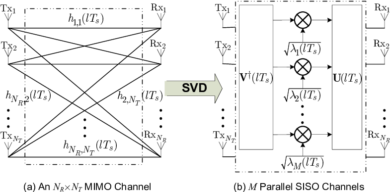
Refer to caption
Figure 1: (aa) A MIMO channel with NTN_{\!T} transmit and NRN_{\!R} receive antennas; (bb) The equivalent MM parallel SISO channel representation.
Refer to caption
Figure 2: The AoA distributions for two scattering examples and the corresponding channel correlation coefficients.
Refer to caption
Figure 3: The correlation coefficient and the LCR of an eigen-channel, in 4×44\times 4 and 12×312\times 3 MIMO systems with isotropic scattering.
Refer to caption
Figure 4: The correlation coefficient and the LCR of an eigen-channel, in 4×44\times 4 and 12×312\times 3 MIMO systems with nonisotropic scattering.
Refer to caption
Figure 5: The correlation coefficient and the LCR of the MIMO IMI at low- and high-SNR regimes, in 4×44\times 4 and 12×312\times 3 MIMO systems with isotropic scattering.
Refer to caption
Figure 6: The correlation coefficient and the LCR of the MIMO IMI at low- and high-SNR regimes, in 4×44\times 4 and 12×312\times 3 MIMO systems with nonisotropic scattering.
Refer to caption
Figure 7: The correlation coefficient of the MIMO IMI at η=15\eta=15 dB (moderate SNR), in a 4×44\times 4 system with isotropic scattering.