{bottomstuff}

This is a revised and extended version of [24] and [26].
Stijn Heymans is supported by the European Commission under the projects Knowledge Web and SUPER; by the FFG (Österreichische Forschungsförderungsgeselleschaft mbH) under the projects RW², SemNetMan, and SEnSE. Davy Van Nieuwenborgh is supported by the Flemish Fund for Scientific Research (FWO-Vlaanderen).

Open Answer Set Programming with Guarded Programs

STIJN HEYMANS
Digital Enterprise Research Institute (DERI)
Leopold-Franzens-Universität
Innsbruck Austria
stijn.heymans@deri.org DAVY VAN NIEUWENBORGH and DIRK VERMEIR
Dept. of Computer Science
Vrije Universiteit Brussel VUB
Pleinlaan 2 B1050 Brussels Belgium
{dvnieuwe dvermeir}@vub.ac.be

Abstract

Open answer set programming (OASP) is an extension of answer set programming where one may ground a program with an arbitrary superset of the program’s constants. We define a fixed point logic (FPL) extension of Clark’s completion such that open answer sets correspond to models of FPL formulas and identify a syntactic subclass of programs, called (loosely) guarded programs. Whereas reasoning with general programs in OASP is undecidable, the FPL translation of (loosely) guarded programs falls in the decidable (loosely) guarded fixed point logic ( $\mu\mbox{(L)GF}$ ). Moreover, we reduce normal closed ASP to loosely guarded OASP, enabling for the first time, a characterization of an answer set semantics by $\mu\mbox{LGF}$ formulas. We further extend the open answer set semantics for programs with generalized literals. Such generalized programs (gPs) have interesting properties, e.g., the ability to express infinity axioms. We restrict the syntax of gPs such that both rules and generalized literals are guarded. Via a translation to guarded fixed point logic, we deduce 2-exptime-completeness of satisfiability checking in such guarded gPs (GgPs). Bound GgPs are restricted GgPs with exptime-complete satisfiability checking, but still sufficiently expressive to optimally simulate computation tree logic (CTL). We translate Datalog lite programs to GgPs, establishing equivalence of GgPs under an open answer set semantics, alternation-free $\mu\mbox{GF}$ , and Datalog lite.

Keywords:

Theory

keywords

Logic Programming

keywords

Answer Set Programming, Open Domains, Fixed Point Logic

1 Introduction

In closed answer set programming (ASP) [14], a program consisting of a rule $\mathit{p(X)}\leftarrow\mathit{not~q(X)}$ and a fact $q(a)$ is grounded with the program’s constant $a$ , yielding $\mathit{p(a)}\leftarrow\mathit{not~q(a)}$ and $q(a)$ . This program has one answer set $\{q(a)\}$ such that one concludes that the predicate $p$ is not satisfiable, i.e., there is no answer set of the program that contains a literal with predicate $p$ . Adding more constants to the program could make $p$ satisfiable, e.g., in the absence of a deducible $q(b)$ , one has $p(b)$ . However, in the context of conceptual modeling, such as designing database schema constraints, this implicit dependence on constants in the program in order to reach sensible conclusions is infeasible. One wants to be able to test satisfiability of a predicate $p$ in a schema independent of any associated data, see, e.g., conceptual modeling as in the Object-role Modeling paradigm [23].

For answer set programming, this problem was solved in [15], where $k$ -belief sets are the answer sets of a program that is extended with $k$ extra constants (reasoning with $k$ -belief sets was shown to be undecidable in [43]). We extended this idea, e.g., in [25], by allowing for arbitrary, thus possibly infinite, universes¹¹ 1 Note that answer sets for programs with (infinite) universes were also considered in [44]. . Open answer sets are pairs $(U,M)$ with $M$ an answer set of the program grounded with $U$ . The above program has an open answer set $(\{x,a\},\{q(a),p(x)\})$ where $p$ is satisfiable. Open Answer Set Programming solves the above conceptual modeling problem, confirmed by the ability of Open Answer Set Programming to simulate several expressive Description Logics [25]. Moreover, as it is a rule-based formalism Open Answer Set Programming is thus very suitable to function as an integrating formalism of Description Logics and Logic Programming.

Characteristic about (O)ASP is its treatment of negation as failure (naf): one guesses an interpretation for a program, computes the program without naf (the GL-reduct [14]), calculates the iterated fixed point of this reduct, and checks whether this fixed point equals the initial interpretation. We compile these external manipulations, i.e., not expressible in the language of programs itself, into fixed point logic (FPL) [21] formulas. First, we rewrite an arbitrary program as a program containing only one designated predicate $p$ and (in)equality; this makes sure that when calculating a fixed point of the predicate variable $p$ , it constitutes a fixed point of the whole program. In the next phase, such a $p$ -program $P$ is translated to FPL formulas $\mathtt{comp}(P)$ . $\mathtt{comp}(P)$ ensures satisfiability of program rules by formulas comparable to those in Clark’s completion. The specific answer set semantics is encoded by formulas indicating that for each atom $p(\textbf{x})$ in the model there must be a true rule body that motivates the atom, and this in a minimal way, i.e., using a fixed point predicate. Negation as failure is correctly handled by making sure that only those rules that would be present in the GL-reduct can be used to motivate atoms.

In [6], Horn clauses were translated to FPL formulas and in [16] reasoning with an extension of stratified Datalog is reduced to FPL, but, to the best of our knowledge, this is the first encoding of an answer set semantics in FPL.

In [36, 31], ASP with (finite) propositional programs is reduced to propositional satisfiability checking. The translation makes the loops in a program explicit and ensures that atoms $p(\textbf{x})$ are motivated by bodies outside of these loops. Although this is an elegant characterization of answer sets in the propositional case, the approach does not seem to hold for OASP, where programs are not propositional but possibly ungrounded and with infinite universes. Instead, we directly use the built-in “loop detection” mechanism of FPL, which enables us to go beyond propositional programs.

Translating OASP to FPL is thus interesting in its own right, but it also enables the analysis of decidability of OASP via decidability results of fragments of FPL. Satisfiability checking of a predicate $p$ w.r.t. a program, i.e., checking whether there exists an open answer set containing some $p(\textbf{x})$ , is undecidable. It is well-known that satisfiability checking in FOL is undecidable, and thus the extension to FPL is too[39]. However, expressive decidable fragments of FPL have been identified [21]: (loosely) guarded fixed point logic ( $\mu\mbox{(L)GF}$ ) extends the (loosely) guarded fragment (L)GF of FOL with fixed point predicates.

GF is identified in [2] as a fragment of FOL satisfying properties such as decidability of reasoning and the tree model property, i.e., every model can be rewritten as a tree model. The restriction of quantified variables by a guard, an atom containing the variables in the formula, ensures decidability in GF. Guards are responsible for the tree model property of GF (where the concept of tree is adapted for predicates with arity larger than $2$ ), which in turn enables tree-automata techniques for showing decidability of satisfiability checking. In [49], GF is extended to LGF where guards can be conjunctions of atoms and, roughly, every pair of variables must be together in some atom in the guard. Satisfiability checking in both GF and LGF is 2-exptime-complete [17], as are their extensions with fixed point predicates $\mu\mbox{GF}$ and $\mu\mbox{LGF}$ [21].

We identify a syntactically restricted class of programs, (loosely) guarded programs ((L)GPs), for which the FPL translation falls in (alternation-free²² 2 $\mu\mbox{(L)GF}$ without nested fixed point variables in alternating least and greatest fixed point formulas.) $\mu\mbox{(L)GF}$ , making satisfiability checking w.r.t. (L)GPs decidable and in 2-exptime. In LGPs, rules have a set of atoms, the guard, in the positive body, such that every pair of variables in the rule appears together in an atom in that guard. GPs are the restriction of LGPs where guards must consist of exactly one atom.

Programs under the normal answer set semantics can be rewritten as LGPs under the open answer set semantics by guarding all variables with atoms that can only introduce constants from the original program. Besides the desirable property that OASP with LGPs is thus a proper decidable extension of normal ASP, this yields that satisfiability checking w.r.t. LGPs is, at least, nexptime-hard.

Datalog lite [16] is a language based on stratified Datalog with input predicates where rules are monadic or guarded and may have generalized literals in the body, i.e., literals of the form ${\FORALL\textbf{Y}}\SUCHTHAT\mathit{a}\Rightarrow\mathit{b}$ for atoms $a$ and $b$ . It has an appropriately adapted bottom-up fixed point semantics. Datalog lite is devised to ensure linear time model checking while being expressive enough to capture computational tree logic [11] and alternation-free $\mu$ -calculus [30]. Moreover, it is shown to be equivalent to alternation-free $\mu\mbox{GF}$ . Our reduction of GPs to alternation-free $\mu\mbox{GF}$ ensures that we have a reduction from GPs to Datalog lite, and thus couples the answer set semantics to a fixed point semantics based on stratified programs. Intuitively, the guess for an interpretation in the answer set semantics corresponds to the input structure one feeds to the stratified Datalog program. The translation from GPs to Datalog lite needs only one stratum to subsequently perform the minimality check of answer set programming.

The other way around, we reduce satisfiability checking in recursion-free Datalog lite to satisfiability checking w.r.t. GPs. Recursion-free Datalog lite is equivalent to GF [16], and, since satisfiability checking of GF formulas is 2-exptime-hard [17], we obtain 2-exptime-completeness for satisfiability checking w.r.t. (L)GPs.

We next extend programs with generalized literals, resulting in generalized programs (gPs). A generalized literal is a first-order formula of the form ${\FORALL\textbf{Y}}\SUCHTHAT\phi\Rightarrow\psi$ where Y is a sequence of variables, $\phi$ is a finite boolean combination of atomic formula and $\psi$ is an atom. Intuitively, such a generalized literal is true in an open interpretation $(U,M)$ if for all substitutions³³ 3 As usual, for a finite boolean combination of atomic formula $\xi$ , we use $\xi[\textbf{Y}\mid\textbf{y}]$ to denote the formula $\xi$ where all occurrences of $Y$ are replaced by $y$ . $[\textbf{Y}\mid\textbf{y}]$ , y in $U$ , such that $\phi[\textbf{Y}\mid\textbf{y}]$ is true in $M$ , $\psi[\textbf{Y}\mid\textbf{y}]$ is true in $M$ .

Generalized literals ${\FORALL\textbf{Y}}\SUCHTHAT\phi\Rightarrow\psi$ , with $\phi$ an atom instead of a finite boolean combination of atomic formula, were introduced in Datalog⁴⁴ 4 The extension of logic programming syntax with first-order formulas dates back to [37]. with the language Datalog lite. In open answer set programming (OASP), we define a reduct that removes the generalized literals. E.g., a rule

r:\mathit{ok}\leftarrow\mathit{{\FORALL X}\SUCHTHAT critical(X)\Rightarrow work(X)}

expresses that a system is OK if all critical devices are functioning: the GeLi-reduct (generalized literal reduct) of such a rule for an open interpretation $(\{x_{0},\ldots\},M)$ where $M$ contains $\mathit{critical(x_{i})}$ for even $i$ , contains a rule

r^{\prime}:\mathit{ok}\leftarrow\mathit{work(x_{0}),work(x_{2}),\ldots}

indicating that the system is OK if the critical devices $x_{0}$ , $x_{2},\ldots$ are working. The GeLi-reduct does not contain generalized literals and one can apply the normal answer set semantics, modified to take into account the infinite body.

Just as it is not feasible to introduce all relevant constants in a program to ensure correct conceptual reasoning, it is not feasible, not even possible, to write knowledge directly as in $r^{\prime}$ for it has an infinite body. Furthermore, even in the presence of a finite universe, generalized literals allow for a more robust representation of knowledge than would be possible without them. E.g., with critical devices $y_{1}$ and $y_{2}$ , a rule $s:\mathit{ok}\leftarrow\mathit{work(y_{1}),work(y_{2})}$ does the job as well as $r$ (and in fact $s$ is the GeLi-reduct of $r$ ), but adding new critical devices, implies revisiting $s$ and replacing it by a rule that reflects the updated situation. Not only is this cumbersome, it may well be impossible as $s$ contains no explicit reference to critical devices, and the knowledge engineer may not have a clue as to which rules to modify.

One can modify the aforementioned FPL translation of programs without generalized literals to take into account generalized literals. With this FPL translation, we then have again a mapping from one undecidable framework into another undecidable framework. We restrict gPs, resulting in guarded gPs (GgPs), such that all variables in a rule appear in an atom in the positive body and all generalized literals are guarded, where a generalized literal is guarded if it can be written as a guarded formula in $\mu\mbox{GF}$ . The FPL translation of GgPs then falls into the $\mu\mbox{GF}$ fragment, yielding a 2-exptime upper complexity bound for satisfiability checking. Together with the 2-exptime-completeness of guarded programs without generalized literals this establishes 2-exptime-completeness for satisfiability checking w.r.t. GgPs. As a consequence, adding generalized literals to a guarded program does not increase the complexity of reasoning.

We further illustrate the expressiveness of (bound) GgPs by simulating reasoning in computational tree logic (CTL) [10], a temporal logic. Temporal logics [10] are widely used for expressing properties of nonterminating programs. Transformation semantics, such as Hoare’s logic are not appropriate here since they depend on the program having a final state that can be verified to satisfy certain properties. Temporal logics on the other hand have a notion of (infinite) time and may express properties of a program along a time line, without the need for that program to terminate. E.g., formulas may express that from each state a program should be able to reach its initial state: $\mathsf{A}\mathsf{G}\mathsf{E}\mathsf{F}\mathit{initial}$ .

Two well-known temporal logics are linear temporal logic (LTL) [10, 45] and computation tree logic (CTL) [10, 12, 8], which differ in their interpretation of time: the former assumes that time is linear, i.e., for every state of the program there is only one successor state, while time is branching for the latter, i.e., every state may have different successor states, corresponding to nondeterministic choices for the program.

Since CTL satisfiability checking is exptime-complete and satisfiability checking w.r.t. GgPs is 2-exptime-complete, a reduction from CTL to GgPs does not seem to be optimal. However, we can show that the particular translation has a special form, i.e., it is bound, for which reasoning is exptime-complete and thus optimal.

Finally, we can reduce general Datalog lite reasoning, i.e., with recursion, to reasoning with GgPs. In particular, we prove a generalization of the well-known result from [14] that the unique answer set of a stratified program coincides with its least fixed point model: for a universe $U$ , the unique open answer set $(U,M)$ of a stratified Datalog program with generalized literals is identical⁵⁵ 5 Modulo equality atoms, which are implicit in OASP, but explicit in Datalog lite. to its least fixed point model with input structure $\mathit{id}{(U)}$ , the identity relation on $U$ . Furthermore, the Datalog lite simulation, together with the reduction of GgPs to alternation-free $\mu\mbox{GF}$ , as well as the equivalence of alternation-free $\mu\mbox{GF}$ and Datalog lite [16], lead to the conclusion that alternation-free $\mu\mbox{GF}$ , Datalog lite, and OASP with GgPs, are equivalent, i.e., their satisfiability checking problems can be effectively polynomially reduced to one another.

GgPs are thus just as expressive as Datalog lite, however, from a knowledge representation viewpoint, GgPs allow for a compact expression of circular knowledge. E.g., the omni-present construction with rules $\mathit{a(X)}\leftarrow\mathit{not~b(X)}$ and $\mathit{b(X)}\leftarrow\mathit{not~a(X)}$ is not stratified and cannot be (directly) expressed in Datalog lite. The reduction to Datalog lite does indicate that negation as failure under the (open) answer set semantics is not that special, but can be regarded as convenient semantic sugar.

The remainder of the paper starts with an introduction of the open answer set semantics, fixed point logic, and computation tree logic. In Section 3, we reduce satisfiability checking w.r.t. arbitrary logic programs to satisfiability checking of alternation-free fixed point logic formulas. We identify in Section 4 syntactical classes of programs for which this FPL translation falls into the decidable logic $\mu\mbox{GF}$ or $\mu\mbox{LGF}$ , i.e., guarded or loosely guarded fixed point logic.

In Section 5, we introduce so-called generalized literals and modify the translation to FPL in Section 6. Section 7 mirrors Section 4 and identifies classes of programs with generalized literals that can be mapped to guarded FPL. In Section 8, we relate the obtained languages under the open answer set semantics to Datalog lite which has a least fixed point model semantics. Section 9 discusses a translation from CTL to bound guarded programs. Finally, Section 10 contains conclusions and directions for further research.

2 Preliminaries

2.1 Open Answer Set Programming

We introduce open answer set programming (OASP) as in [27]. Constants, variables, terms, and atoms are defined as usual⁶⁶ 6 Note that we do not allow function symbols. . A literal is an atom $p(\textbf{t})$ or a naf-atom $not~p(\textbf{t})$ .⁷⁷ 7 We have no classical negation $\neg$ , however, programs with $\neg$ can be reduced to programs without it, see e.g. [33]. The positive part of a set of literals $\alpha$ is ${\alpha}^{+}=\{p(\textbf{t})\mid p(\textbf{t})\in\alpha\}$ and the negative part of $\alpha$ is ${\alpha}^{-}=\{p(\textbf{t})\mid not~p(\textbf{t})\in\alpha\}$ . We assume the existence of binary predicates $=$ and $\neq$ , where $t=s$ is considered as an atom and $t\neq s$ as $not~t=s$ . E.g., for $\alpha=\{X\neq Y,Y=Z\}$ , we have ${\alpha}^{+}=\{Y=Z\}$ and ${\alpha}^{-}=\{X=Y\}$ . A regular atom is an atom that is not an equality atom. For a set $X$ of atoms, $not~X=\{not~l\mid l\in X\}$ .

A program is a countable set of rules $\mathit{\alpha}\leftarrow\mathit{\beta}$ , where $\alpha$ and $\beta$ are finite sets of literals, $\mbox{$|{\alpha}^{+}|$}\leq 1$ , and ${\FORALL t,s}\SUCHTHAT t=s\not\in{{\alpha}^{+}}$ , i.e., $\alpha$ contains at most one positive atom, and this atom cannot be an equality atom.⁸⁸ 8 The condition $\mbox{$|{\alpha}^{+}|$}\leq 1$ ensures that the GL-reduct is non-disjunctive. The set $\alpha$ is the head of the rule and represents a disjunction of literals, while $\beta$ is called the body and represents a conjunction of literals. If $\alpha=\emptyset$ , the rule is called a constraint. Free rules are rules of the form $\mathit{q(\textbf{t})\lor not~q(\textbf{t})}\leftarrow\mathit{}$ for a tuple t of terms; they enable a choice for the inclusion of atoms. We call a predicate $p$ free if there is a free rule $\mathit{p(\textbf{t})\lor not~p(\textbf{t})}\leftarrow\mathit{}$ . Atoms, literals, rules, and programs that do not contain variables are ground.

For a program $P$ , let $\mathit{cts}{(P)}$ be the constants in $P$ , $\mathit{vars}(P)$ its variables, and $\mathit{preds}(P)$ its predicates. A universe $U$ for $P$ is a non-empty countable⁹⁹ 9 Note that $U$ is countable, as later on, this is needed to be able to use a result from [17] that indicates that the fixed point can be reached at the first ordinal $\omega$ . superset of the constants in $P$ : $\mathit{cts}{(P)}\subseteq U$ . We call ${P}_{U}$ the ground program obtained from $P$ by substituting every variable in $P$ by every possible constant in $U$ . Let $\mathcal{B}_{P}^{U}$ be the set of ground regular atoms that can be formed from a ground program $P$ and the elements in $U$ .

Let $I$ be a subset of some $\mathcal{B}_{P}^{U}$ . For a ground regular atom $p(\textbf{t})$ , we write $I\models p(\textbf{t})$ if $p(\textbf{t})\in I$ ; For an equality atom $p(\textbf{t})\equiv t=s$ , we have $I\models p(\textbf{t})$ if $s$ and $t$ are equal constants. We have $I\models not~p(\textbf{t})$ if $I\not\models p(\textbf{t})$ . For a set of ground literals $X$ , $I\models X$ if $I\models l$ for every $l\in X$ . A ground rule $r:\mathit{\alpha}\leftarrow\mathit{\beta}$ is satisfied w.r.t. $I$ , denoted $I\models r$ , if $I\models l$ for some $l\in\alpha$ whenever $I\models\beta$ . A ground constraint $\mathit{}\leftarrow\mathit{\beta}$ is satisfied w.r.t. $I$ if $I\not\models\beta$ . For a ground program $P$ without not, $I$ is a model of $P$ if $I$ satisfies every rule in $P$ ; it is an answer set of $P$ if it is a subset minimal model of $P$ . For ground programs $P$ containing not, the GL-reduct [14] w.r.t. $I$ is defined as $P^{I}$ , where $P^{I}$ contains $\mathit{{\alpha}^{+}}\leftarrow\mathit{{\beta}^{+}}$ for $\mathit{\alpha}\leftarrow\mathit{\beta}$ in $P$ , $I\models not~{\beta}^{-}$ and $I\models{\alpha}^{-}$ . $I$ is an answer set of a ground $P$ if $I$ is an answer set of $P^{I}$ .

In the following, a program is assumed to be a finite set of rules; infinite programs only appear as byproducts of grounding a finite program with an infinite universe. An open interpretation of a program $P$ is a pair $(U,M)$ where $U$ is a universe for $P$ and $M$ is a subset of $\mathcal{B}_{P}^{U}$ . An open answer set of $P$ is an open interpretation $(U,M)$ of $P$ with $M$ an answer set of ${P}_{U}$ . An $n$ -ary predicate $p$ in $P$ is satisfiable if there is an open answer set $(U,M)$ of $P$ and a $\textbf{x}\in U^{n}$ such that $p(\textbf{x})\in M$ . We assume that when satisfiability checking a predicate $p$ , $p$ is always non-free, i.e., there are no free rules with $p$ in the head. Note that satisfiability checking of a free $n$ -ary predicate $p$ w.r.t. $P$ can always be reduced to satisfiability checking of a new non-free $n$ -ary predicate $p^{\prime}$ w.r.t. $P\cup\{\mathit{p^{\prime}(\textbf{X})}\leftarrow\mathit{p(\textbf{X})}\}$ . Note that this is a linear reduction.

Example 2.1.

Take the program

\begin{array}[]{rrll}\mathit{r_{1}}:&\mathit{restore(X)}&\leftarrow&\mathit{crash(X),y(X,Y),backSucc(Y)}\\ \mathit{r_{2}}:&\mathit{backSucc(X)}&\leftarrow&\mathit{\neg crash(X),y(X,Y),not~backFail(Y)}\\ \mathit{r_{3}}:&\mathit{backFail(X)}&\leftarrow&\mathit{not~backSucc(X)}\\ \mathit{r_{4}}:&\mathit{}&\leftarrow&\mathit{{y}(Y_{1},X),{y}(Y_{2},X),Y_{1}\neq Y_{2}}\\ \mathit{r_{5}}:&\mathit{y(X,Y)\lor not~y(X,Y)}&\leftarrow&\mathit{}\\ \mathit{r_{6}}:&\mathit{crash(X)\lor not~crash(X)}&\leftarrow&\mathit{}\\ \mathit{r_{7}}:&\mathit{\neg crash(X)\lor not~\neg crash(X)}&\leftarrow&\mathit{}\\ \end{array}

Rule $r_{1}$ represents the knowledge that a system that has crashed on a particular day $X$ ( $\mathit{crash(X)}$ ), can be restored on that day ( $\mathit{restore(X)}$ ) if a backup of the system on the day $Y$ before ( $\mathit{y(X,Y)}$ – $\mathit{y}$ stands for yesterday) succeeded ( $\mathit{backSucc(Y)}$ ). Backups succeed, if the system does not crash and it cannot be established that the backups at previous dates failed ( $r_{2}$ ) and a backup fails if it does not succeed ( $r_{3}$ ). Rule $r_{4}$ ensures that for a particular today there can be only one tomorrow. Rules $r_{5}$ , $r_{6}$ , and $r_{7}$ allow to freely introduce $\mathit{y}$ , $\mathit{crash}$ , and $\mathit{\neg crash}$ literals. Indeed, take, e.g., $\mathit{crash(x)}$ in an interpretation; the GL-reduct w.r.t. that interpretation contains then the rule $\mathit{crash(x)}\leftarrow\mathit{}$ which motivates the presence of the $\mathit{crash}$ literal in an (open) answer set. If there is no $\mathit{crash(x)}$ in an interpretation then the GL-reduct removes the rule $r_{5}$ (more correctly, its grounded version with $x$ ). Below, we formally define rules of such a form as free rules in correspondence with the intuition that they allow for a free introduction of literals.

Every open answer set $(U,M)$ of this program that makes $\mathit{restore}$ satisfiable, i.e., such that there is a $\mathit{restore(x)\in M}$ for some $x\in U$ , must be infinite. An example of such an open answer set $M$ is (we omit $U$ if it is clear from $M$ )

\{restore(x),crash(x),backFail(x),y(x,x_{1}),\\ backSucc(x_{1}),\lnot crash(x_{1}),y(x_{1},x_{2})\\ backSucc(x_{2}),\lnot crash(x_{2}),y(x_{2},x_{3}),\ldots\}

One sees that every $\mathit{backSucc}$ literal with element $x_{i}$ enforces a new $\mathit{y}$ -successor $x_{i+1}$ since none of the previously introduced universe elements can be used without violating rule $r_{4}$ , thus enforcing an infinite open answer set.

Indeed, assume $\mathit{restore}$ is satisfiable w.r.t. $P$ . Then, there must be a $x_{0}$ in the universe $U$ of some open answer set $(U,M)$ such that $\mathit{restore(x_{0})}\in M$ . With $r_{1}$ , we must have that $\mathit{crash(x_{0})}\in M$ , and there must be some $x_{1}\in U$ such that $\mathit{y(x_{0},x_{1})}\in M$ and $\mathit{backSucc(x_{1})}\in M$ , and thus, with rule $r_{2}$ , $\mathit{\neg crash(x_{1})}\in M$ , $\mathit{y(x_{1},x_{2})}\in M$ and $\mathit{backFail(x_{2})}\not\in M$ . With $\mathit{crash(x_{0})}\in M$ and $\neg\mathit{crash(x_{1})}\in M$ , we are sure that $x_{1}\neq x_{0}$ . With $r_{3}$ , one must have that $\mathit{backSucc(x_{2})}\in M$ such that $x_{2}\neq x_{0}$ for the same reason. Furthermore, $x_{2}\neq x_{1}$ , since otherwise $\mathit{y(x_{0},x_{1})}\in M$ and $\mathit{y(x_{1},x_{1})}\in M$ : with $x_{0}\neq x_{1}$ this is a contradiction with $r_{4}$ . Thus, summarizing, $x_{2}\neq x_{1}$ and $x_{2}\neq x_{0}$ . One can continue this way, and one will be obliged to introduce new $x_{i}$ ’s ad infinitum.

Rules $\mathit{\alpha}\leftarrow\mathit{\beta}$ are such that $\mbox{$|{\alpha}^{+}|$}\leq 1$ . This restriction ensures that the GL-reduct contains no disjunction in the head anymore, i.e., the head will be an atom or it will be empty. This property of the GL-reduct allows us to define an immediate consequence operator [50] $T$ that computes the closure of a set of literals w.r.t. a GL-reduct.

For a program $P$ and an open interpretation $(U,M)$ of $P$ , $T_{P}^{(U,M)}:\mathcal{B}_{P_{U}}\to\mathcal{B}_{P_{U}}$ is defined as $T(B)=B\cup\{a\mid a\leftarrow\beta\in P_{U}^{M}\land B\models\beta\}$ . Additionally, we define $T^{0}(B)=B$ , and $T^{n+1}(B)=T(T^{n}(B))$ .¹⁰¹⁰ 10 We omit the sub- and superscripts $(U,M)$ and $P$ from $T_{P}^{(U,M)}$ if they are clear from the context and, furthermore, we will usually write $T$ instead of $T(\emptyset)$ .

Although we allow for infinite universes, we can motivate the presence of atoms in open answer sets in a finite way, where the motivation of an atom is formally expressed by the immediate consequence operator.

Theorem 2.2

Let $P$ be a program and $(U,M)$ an open answer set of $P$ . Then, ${\FORALL a\in M}\SUCHTHAT{\EXISTS n<\infty}\SUCHTHAT a\in T^{n}$ .

For the relation of OASP with other logic programming paradigms that allow for (some form of) opennes, we refer to [27].

2.2 Fixed Point Logic

Extensions of first-order logic (FOL) that allow for the expression of recursive procedures are well-investigated in finite model theory, see e.g., [39, 29]. Also in the presence of infinite models, so-called fixed point logic (FPL) proves to be an interesting logic [13]. E.g., a decidable subclass of FPL is the guarded fixed point logic [21], which lifts propositional $\mu$ -calculus [30] to a first-order setting.

We assume FOL interpretations are represented as pairs $(U,M)$ where $M$ is an interpretation over the domain $U$ . Furthermore, we consider FOL with equality such that equality is always interpreted as the identity relation over $U$ .

We define fixed point logic (FPL) along the lines of [21], i.e., as an extension of first-order logic, where formulas may additionally be fixed point formulas of the form

[\mathrm{LFP}~{W}{\textbf{X}}.{\psi(W,\textbf{X})}](\textbf{X})\quad\mbox{ or }\quad[\mathrm{GFP}~{W}{\textbf{X}}.{\psi(W,\textbf{X})}](\textbf{X})\;,

(1)

where $W$ is an $n$ -ary predicate variable, X is an $n$ -ary sequence of distinct variables, $\psi(W,\textbf{X})$ is a (FPL) formula with all free variables contained in X and $W$ appears only positively in $\psi(W,\textbf{X})$ .¹¹¹¹ 11 A formula $\psi$ is in negation-normal form if the only used connectives are $\land$ , $\lor$ , and $\neg$ , and $\neg$ only appears in front of atoms. Let $\psi$ be a formula in negation-normal form. A predicate $p$ appears then only positively in $\psi$ if there is no $\neg p$ in $\psi$ .

For an interpretation $(U,M)$ and a valuation $\chi$ of the free predicate variables, except $W$ , in $\psi$ , we define the operator $\psi^{(U,M),\chi}:2^{U^{n}}\to 2^{U^{n}}$ on sets $S$ of $n$ -ary tuples

\psi^{(U,M),\chi}(S)\equiv\{\textbf{x}\in U^{n}\mid(U,M),\chi\cup\{W\to S\}\models\psi(W,\textbf{x})\}\;,

(2)

where $\chi\cup\{W\to S\}$ is the valuation $\chi$ extended such that the extension of $W$ is assigned to $S$ . If $\psi(W,\textbf{X})$ contains only the predicate variable $W$ , we often omit the valuation $\chi$ and write just $\psi^{(U,M)}$ . By definition, $W$ appears only positively in $\psi$ such that $\psi^{(U,M),\chi}$ is monotonic on sets of $n$ -ary $U$ -tuples and thus has a least and greatest fixed point [47], which we denote by $\mathrm{LFP}({\psi^{(U,M),\chi}})$ and $\mathrm{GFP}({\psi^{(U,M),\chi}})$ respectively. Finally, we have that

(U,M),\chi\models[\mathrm{LFP}~{W}{\textbf{X}}.{\psi(W,\textbf{X})}](\textbf{x})\iff\textbf{x}\in\mathrm{LFP}({\psi^{(U,M),\chi}})\;,

(3)

and similarly for greatest fixed point formulas. We call an FPL sentence (i.e., an FPL formula without free variables) alternation-free if it does not contain subformulas $\psi\equiv[\mathrm{LFP}~{T}{\textbf{X}}.{\varphi}](\textbf{X})$ and $\theta\equiv[\mathrm{GFP}~{S}{\textbf{Y}}.{\eta}](\textbf{Y})$ such that $T$ occurs in $\eta$ and $\theta$ is a subformula of $\varphi$ , or $S$ occurs in $\varphi$ and $\psi$ is a subformula of $\eta$ . We can eliminate greatest fixed point formulas from a formula, by the equivalence:

[\mathrm{GFP}~{W}{\textbf{X}}.{\psi}]\equiv\neg[\mathrm{LFP}~{W}{\textbf{X}}.{\neg\psi[W/\neg W]}]\;,

(4)

where $\neg\psi[W/\neg W]$ is $\neg\psi$ with $W$ replaced by $\neg W$ . If we thus remove greatest fixed point predicates, and if negations appear only in front of atoms or least fixed point formulas, then a formula is alternation-free iff no fixed point variable $W$ appears in the scope of a negation.

As in [18], we define

\begin{split}\psi^{(U,M)}\uparrow 0&\equiv\emptyset\\ \psi^{(U,M)}\uparrow\alpha+1&\equiv\psi^{(U,M)}(\psi^{(U,M)}\uparrow\alpha)\text{ for ordinals $\alpha$}\\ \psi^{(U,M)}\uparrow\beta&\equiv\bigcup_{\alpha<\beta}(\psi^{(U,M)}\uparrow\alpha)\text{ for limit ordinals $\beta$}\end{split}

Furthermore, since $\psi^{(U,M)}$ is monotone, we have that $\psi^{(U,M)}\uparrow 0\subseteq\psi^{(U,M)}\uparrow 1\subseteq\ldots$ and there exists a (limit) ordinal $\alpha$ such that $\psi^{(U,M)}\uparrow\alpha=\mathrm{LFP}({\psi^{(U,M)}})$ .

Example 2.3.

Take the conjunction of the following formulas, i.e., the infinity axiom¹²¹² 12 An infinity axiom is a formula that has only infinite models (if it has models). from [21]:

	$\displaystyle{\EXISTS X,Y}\SUCHTHAT F(X,Y)$		(5)
	$\displaystyle{\FORALL X,Y}\SUCHTHAT\left(F(X,Y)\Rightarrow({\EXISTS Z}\SUCHTHAT F(Y,Z))\right)$		(6)
	$\displaystyle{\FORALL X,Y}\SUCHTHAT F(X,Y)\Rightarrow[\mathrm{LFP}~{W}{X}.{{\FORALL Y}\SUCHTHAT F(Y,X)\Rightarrow W(Y)}](X)$		(7)

A model of these formulas contains at least one $F(x,y)$ (by formula (5)), which then leads to a $F$ -chain by formula (6). Formula (7) ensures that each element $x$ is on a well-founded chain (and thus formula (6) actually generates an infinite chain).

2.3 Computation Tree Logic

We introduce in this subsection the temporal logic computation tree logic (CTL) [10, 12, 8]. Let AP be the finite set of available proposition symbols. CTL formulas are defined as follows:

•

every proposition symbol $P\in AP$ is a formula,
•

if $p$ and $q$ are formulas, so are $p\land q$ and $\neg p$ ,
•

if $p$ and $q$ are formulas, then $\mathsf{E}\mathsf{X}p$ , $\mathsf{E}(p~\mathsf{U}~q)$ , $\mathsf{A}\mathsf{X}p$ , and $\mathsf{A}(p~\mathsf{U}~q)$ are formulas.

The semantics of a CTL formula is given by (temporal) structures. A structure $K$ is a tuple $(S,R,L)$ with $S$ a countable set of states, $R\subseteq S\times S$ a total relation in $S$ , i.e., ${\FORALL s\in S}\SUCHTHAT{\EXISTS t\in S}\SUCHTHAT(s,t)\in R$ , and $L:S\to 2^{AP}$ a function labeling states with propositions. Intuitively, $S$ is a set of states, $R$ indicates the permitted transitions between states, and $L$ indicates which propositions are true at certain states.

A path $\pi$ in $K$ is an infinite sequence of states $(s_{0},s_{1},\ldots)$ such that $(s_{i-1},s_{i})\in R$ for each $i>0$ . For a path $\pi=(s_{0},s_{1},\ldots)$ , we denote the element $s_{i}$ with $\pi_{i}$ . For a structure $K=(S,R,L)$ , a state $s\in S$ , and a formula $p$ , we inductively define when $K$ is a model of $p$ at $s$ , denoted $K,s\models p$ :

•

$K,s\models P$ iff $P\in L(s)$ for $P\in AP$ ,
•

$K,s\models\neg p$ iff not $K,s\models p$ ,
•

$K,s\models p\land q$ iff $K,s\models p$ and $K,s\models q$ ,
•

$K,s\models\mathsf{E}\mathsf{X}p$ iff there is a $(s,t)\in R$ and $K,t\models p$ ,
•

$K,s\models\mathsf{A}\mathsf{X}p$ iff for all $(s,t)\in R$ , $K,t\models p$ ,
•

$K,s\models\mathsf{E}(p~\mathsf{U}~q)$ iff there exists a path $\pi$ in $K$ with $\pi_{0}=s$ and ${\EXISTS k\geq 0}\SUCHTHAT(K,\pi_{k}\models q\land{\FORALL j<k}\SUCHTHAT K,\pi_{j}\models p)$ ,
•

$K,s\models\mathsf{A}(p~\mathsf{U}~q)$ iff for all paths $\pi$ in $K$ with $\pi_{0}=s$ we have ${\EXISTS k\geq 0}\SUCHTHAT(K,\pi_{k}\models q\land{\FORALL j<k}\SUCHTHAT K,\pi_{j}\models p)$ .

Intuitively, $K,s\models\mathsf{E}\mathsf{X}p$ ( $K,s\models\mathsf{A}\mathsf{X}p$ ) can be read as “there is some neXt state where $p$ holds” (“ $p$ holds in all next states”), and $K,s\models\mathsf{E}(p~\mathsf{U}~q)$ ( $K,s\models\mathsf{A}(p~\mathsf{U}~q)$ ) as “there is some path from $s$ along which $p$ holds Until $q$ holds (and $q$ eventually holds)” (“for all paths from $s$ , $p$ holds until $q$ holds (and $q$ eventually holds)”).

Some common abbreviations for CTL formulas are $\mathsf{E}\mathsf{F}p=\mathsf{E}(true~\mathsf{U}~p)$ (there is some path on which $p$ will eventually hold), $\mathsf{A}\mathsf{F}p=\mathsf{A}(true~\mathsf{U}~p)$ ( $p$ will eventually hold on all paths), $\mathsf{E}\mathsf{G}p=\neg\mathsf{A}\mathsf{F}\neg p$ (there is some path on which $p$ holds globally), and $\mathsf{A}\mathsf{G}p=\neg\mathsf{E}\mathsf{F}\neg p$ ( $p$ holds everywhere on all paths). Furthermore, we have the standard propositional abbreviations $p\lor q=\neg(\neg p\land\neg q)$ , $p\Rightarrow q=\neg p\lor q$ , and $p\Leftrightarrow q=(p\Rightarrow q)\land(q\Rightarrow p)$ .

A structure $K=(S,R,L)$ satisfies a CTL formula $p$ if there is a state $s\in S$ such that $K,s\models p$ ; we also call $K$ a model of $p$ . A CTL formula $p$ is satisfiable iff there is a model of $p$ .

Example 2.4.

Consider the expression of absence of starvation $t\Rightarrow\mathsf{A}\mathsf{F}c$ [8] for a process in a mutual exclusion problem¹³¹³ 13 In the mutual exclusion problem, we have two or more processes that want to access a critical section of code, but cannot do this at the same time. The problem is then how to model the behavior of the processes (or the concurrent program in general), such that this mutual exclusion is never violated. For more details, we refer to, e.g., [11, 10, 8, 3, 28, 38]. . The formula demands that if a process tries ( $t$ ) to enter a critical region, it will eventually succeed in doing so ( $c$ ) for all possible future execution paths.

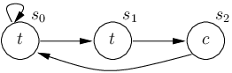
We will usually represent structures by diagrams as in Figure 1, where states are nodes, transitions between nodes define $R$ , and the labels of the nodes contain the propositions true at the corresponding states. E.g., take the structure $K=(S,R,L)$ with

•

$S=\{s_{0},s_{1},s_{2}\}$ ,
•

$R=\{(s_{0},s_{0}),(s_{0},s_{1}),(s_{1},s_{2}),(s_{2},s_{0})\}$ , and
•

$L(s_{0})=L(s_{1})=t$ , $L(s_{2})=c$ ,

which is represented by Figure 1. This structure does not satisfy $t\Rightarrow\mathsf{A}\mathsf{F}c$ at $s_{0}$ since on the path $(s_{0},s_{0},\ldots)$ the proposition $c$ never holds. We have, however, $K,s_{1}\models t\Rightarrow\mathsf{A}\mathsf{F}c$ : $t$ holds at $s_{1}$ such that we must have that on all paths from $s_{1}$ the proposition $c$ must eventually hold; since the only path from $s_{1}$ leads to $s_{2}$ where $c$ holds, $t\Rightarrow\mathsf{A}\mathsf{F}c$ holds at $s_{1}$ . We also have $K,s_{2}\models t\Rightarrow\mathsf{A}\mathsf{F}c$ , since $t\not\in L(s_{2})$ .

Refer to caption — Figure 1: Example Structure $t\Rightarrow\mathsf{A}\mathsf{F}c$

Theorem 2.5 ([10])

The problem of testing satisfiability for CTL is complete for deterministic exponential time.

3 Open Answer Set Programming via Fixed Point Logic

In this section, we will show how the external manipulations to define the (open) answer set semantics can be compiled into fixed point logic, so allowing in the next sections to analyse the decidability of OASP via the various decidability results of fragments of FPL.

We assume, without loss of generality, that the predicates in a program $P$ are differently named than the constants in $P$ and that each predicate $q$ in $P$ has one associated arity, e.g., $q(x)$ and $q(x,y)$ are not allowed.

Definition 3.1.

A program $P$ is a $p$ -program if the only predicate in $P$ different from the (in)equality predicate is $p$ .

For a program $P$ , let $\mathit{in(Y)}\equiv\{Y\neq a\mid a\in\mathit{preds}(P)\cup\{0\}\}$ , i.e., a set of inequalities between the variable $Y$ and the predicates in $P$ as well as a new constant $0$ . For a sequence of variables Y, we have $\mathit{in}(\textbf{Y})\equiv\cup_{Y\in\textbf{Y}}\mathit{in(Y)}$ .

For a predicate name $p$ not appearing in an arbitrary program $P$ , we can rewrite $P$ as an equivalent $p$ -program ${P}_{p}$ by replacing every regular $m$ -ary atom $q(\textbf{t})$ in $P$ by $p(\textbf{t},\textbf{0},q)$ where $p$ has arity $n$ , with $n$ the maximum of the arities of predicates in $P$ augmented by $1$ , 0 is a sequence of new constants $0$ of length $n-m-1$ , and $q$ is a new constant with the same name as the original predicate. Furthermore, in order to avoid grounding with the new constants, we add for every variable $X$ in a non-free rule $r\in P$ and for every newly added constant $a$ in ${P}_{p}$ , $X\neq a$ to the body. The rule in ${P}_{p}$ corresponding to $r:\mathit{\alpha}\leftarrow\mathit{\beta}\in P$ is denoted as ${r}_{p}:\mathit{{\alpha}_{p}}\leftarrow\mathit{{\beta}_{p},\mathit{in(\textbf{X})}}\in{P}_{p}$ for $\mathit{vars}(r)=\mathit{\textbf{X}}$ .

Example 3.2.

Take a program $P$ :

\begin{array}[]{rll}\mathit{h(a,b)}&\leftarrow&\mathit{q(X)}\\ \mathit{q(X)\lor not~q(X)}&\leftarrow&\mathit{}\\ \mathit{}&\leftarrow&\mathit{q(a)}\\ \mathit{}&\leftarrow&\mathit{q(b)}\\ \end{array}

For a universe $U=\{x,a,b\}$ of $P$ , we have the open answer sets $M_{1}=(U,\emptyset)$ and $M_{2}=(U,\{q(x),h(a,b)\})$ . The translation ${P}_{p}$ is

\begin{array}[]{rll}\mathit{p(a,b,h)}&\leftarrow&\mathit{p(X,0,q),X\neq 0,X\neq h,X\neq q}\\ \mathit{p(X,0,q)\lor not~p(X,0,q)}&\leftarrow&\mathit{}\\ \mathit{}&\leftarrow&\mathit{p(a,0,q)}\\ \mathit{}&\leftarrow&\mathit{p(b,0,q)}\\ \end{array}

The open answer sets of this program can then be rewritten as open answer sets of the original program (by leaving out all “wrong” literals $p(q,0,q),p(0,0,q),p(h,0,q)$ that can be generated by the free rule).

Theorem 3.3

Let $P$ be a program, $p$ a predicate not in $P$ , and $q$ a predicate in $P$ . $q$ is satisfiable w.r.t. $P$ iff there is an open answer set $(U^{\prime},M^{\prime})$ of the $p$ -program $P_{p}$ with $p(\textbf{x},\textbf{0},q)\in M^{\prime}$ .

Proof.

For the “only if” direction, assume $(U,M)$ is an open answer set of $P$ that satisfies $q$ , i.e., there is a $q(\textbf{x})\in M$ . Let $U^{\prime}=U\cup\mathit{preds}(P)\cup\{0\}$ and $M^{\prime}=\{p(\textbf{x},\textbf{0},q)\mid q(\textbf{x})\in M\})$ . Then $(U^{\prime},M^{\prime})$ is an open interpretation of $P_{p}$ and $p(\textbf{x},\textbf{0},q)\in M^{\prime}$ . One can show that $(U^{\prime},M^{\prime})$ is an open answer set of $P_{p}$ .

For the “if” direction, assume $(U^{\prime},M^{\prime})$ is an open answer set of ${P}_{p}$ with $p(\textbf{x},\textbf{0},q)\in M^{\prime}$ . Define $U\equiv U^{\prime}\;\!\setminus\!(\mathit{preds}(P)\cup\{0\})$ and $M\equiv\{q(\textbf{x})\mid p(\textbf{x},\textbf{0},q)\in M^{\prime}\land\textbf{x}\cap(\mathit{preds}(P)\cup\{0\})=\emptyset\}$ .

We can assume that $q$ is a non-free predicate (and we assume this throughout the rest of this paper). Then there are no free rules with a $q(\textbf{t})$ in the head such that there are no free rules with a $p(\textbf{t},\textbf{0},q)$ in the head in $P_{p}$ . Since there is a $p(\textbf{x},\textbf{0},q)\in M^{\prime}$ , and $(U^{\prime},M^{\prime})$ is an open answer set, there must be a rule $r[]$ in $({P}_{p})_{U^{\prime}}^{M^{\prime}}$ ¹⁴¹⁴ 14 For objects $o$ (rules, (sets of) literals, …), we denote with $o[Y_{1}|y_{1},\ldots,Y_{d}|y_{d}]$ , the grounding of $o$ where each variable $Y_{i}$ is substituted with $y_{i}$ . Equivalently, we may write $o[\textbf{Y}|\textbf{y}]$ for $\textbf{Y}=Y_{1},\ldots,Y_{d}$ and $\textbf{y}=y_{1},\ldots,y_{d}$ , or $o[]$ if the grounding substitution is clear from the context, or if it does not matter what the substitution exactly looks like. such that $M^{\prime}\models\mathit{in(\textbf{Y})[]}$ for Y the variables in the corresponding ungrounded rule $r$ . Thus $\textbf{x}\cap(\mathit{preds}(P)\cup\{0\})=\emptyset$ , such that $q(\textbf{x})\in M$ , by definition of $M$ .

One can show that $(U,M)$ is an open answer set of $P$ . ∎∎

The translation of a program to a $p$ -program does not influence the complexity of reasoning.

Theorem 3.4

Let $P$ be a program and $p$ a predicate not in $P$ . The size¹⁵¹⁵ 15 In the rest of the paper we use $n\times s$ for the size of a program $P$ , where $n$ is the number of rules in $P$ and $s$ is the maximum size of the rules in $P$ . of ${P}_{p}$ is polynomial in the size of $P$ .

Proof.

The size of a rule $r\in P$ is of the order $v+k$ , with $v$ the number of variables and $k$ the number of predicate names in $r$ . The corresponding $r_{p}$ then contains an extra $v\times n$ inequality atoms for $n\equiv\mbox{$|\mathit{preds}(P)\cup\{0\}|$}$ , and the size of $r_{p}$ is thus in general quadratic in the size of $r$ . ∎∎

By Theorems 3.3 and 3.4, we can focus, without loss of generality, on $p$ -programs only. Since $p$ -programs have open answer sets consisting of one predicate $p$ , fixed points calculated w.r.t. $p$ yield minimal models of the program as we will show in Theorem 3.8.

In [6], a similar motivation drives the reduction of Horn clauses¹⁶¹⁶ 16 Horn clauses are rules of the form $a\leftarrow\beta$ where $\beta$ is a finite set of atoms (i.e., negation as failure is not allowed). to clauses consisting of only one defined predicate. Their encoding does not introduce new constants to identify old predicates and depends entirely on the use of (in)equality. However, to account for databases consisting of only one element, [6] needs an additional transformation that unfolds bodies of clauses.

We can reduce a $p$ -program $P$ to equivalent formulas $\mathtt{comp}(P)$ in fixed point logic. The completion $\mathtt{comp}(P)$ of a program $P$ consists of formulas that demand that different constants in $P$ are interpreted as different elements:

a\neq b

(8)

for every pair of different constants $a$ and $b$ in $P$ , and where $a\neq b\equiv\neg(a=b)$ . $\mathtt{comp}(P)$ contains formulas ensuring the existence of at least one element in the domain of an interpretation:

{\EXISTS X}\SUCHTHAT\textbf{true}\;.

(9)

Besides these technical requirements matching FOL interpretations with open interpretations, $\mathtt{comp}(P)$ contains the formulas in $\mathtt{fix}(P)\equiv\mathtt{sat}(P)\cup\mathtt{gl}(P)\cup\mathtt{fpf}(P)$ , which can be intuitively categorized as follows:

•

$\mathtt{sat}(P)$ ensures that a model of $\mathtt{fix}(P)$ satisfies all rules in $P$ ,
•

$\mathtt{gl}(P)$ is an auxiliary component defining atoms that indicate when a rule in $P$ belongs to the GL-reduct of $P$ , and
•

$\mathtt{fpf}(P)$ ensures that every model of $\mathtt{fix}(P)$ is a minimal model of the GL-reduct in $P$ ; it uses the atoms defined in $\mathtt{gl}(P)$ to select, for the calculation of the fixed point, only those rules in $P$ that are in the GL-reduct of $P$ .

We interpret a naf-atom $not~a$ in a FOL formula as the literal $\neg a$ . Moreover, we assume that, if a set $X$ is empty, $\bigwedge X=\textbf{true}$ and $\bigvee X=\textbf{false}$ . In the following, we assume that the arity of $p$ , the only predicate in a $p$ -program is $n$ .

Definition 3.5.

Let $P$ be a $p$ -program. The fixed point translation of $P$ is $\mathtt{fix}(P)\equiv\mathtt{sat}(P)\cup\mathtt{gl}(P)\cup\mathtt{fpf}(P)$ , where

1.

$\mathtt{sat}(P)$ contains formulas

${\FORALL\textbf{Y}}\SUCHTHAT\bigwedge\beta\Rightarrow\bigvee\alpha$ (10)

for rules $\mathit{\alpha}\leftarrow\mathit{\beta}\in P$ with variables Y,
2.

$\mathtt{gl}(P)$ contains the formulas

${\FORALL\textbf{Y}}\SUCHTHAT\mathit{r(\textbf{Y})}\Leftrightarrow\mathit{\bigwedge{\alpha}^{-}\land\bigwedge\neg{\beta}^{-}}$ (11)

for rules $r:\mathit{\alpha}\leftarrow\mathit{\beta}\in P$ ¹⁷¹⁷ 17 We assume that rules are uniquely named. with variables Y,

$\mathtt{fpf}(P)$ contains the formula

{\FORALL\textbf{X}}\SUCHTHAT\mathit{p(\textbf{X})}\Rightarrow\mathit{[\mathrm{LFP}~{W}{\textbf{X}}.{\phi(W,\textbf{X})}](\textbf{X})}

(12)

with

\phi(W,\textbf{X})\equiv W(\textbf{X})\lor\bigvee_{r:\mathit{p(\textbf{t})\lor\alpha}\leftarrow\mathit{\beta}\in P}E(r)

(13)

and

E(r)\equiv{\EXISTS\textbf{Y}}\SUCHTHAT X_{1}=t_{1}\land\ldots\land X_{n}=t_{n}\land\bigwedge{\beta}^{+}[p|W]\land r(\textbf{Y})

(14)

where $\textbf{X}=X_{1},\ldots,X_{n}$ are $n$ new variables, Y are the variables in $r$ , $W$ is a new (second-order) variable and ${\beta}^{+}[p|W]$ is ${\beta}^{+}$ with $p$ replaced by $W$ .

The completion of $P$ is $\mathtt{comp}(P)\equiv\mathtt{fix}(P)\cup\{(\ref{eq:constants}),(\ref{eq:oneelem})\}$ .

The predicate $W$ appears only positively in $\phi(W,\textbf{X})$ such that the fixed point formula in $(\ref{eq:fpf})$ is well-defined. By the first disjunct in $(\ref{eq:fpformula})$ , we have that applying the operator $\phi^{(U,M)}$ (see pp. 2) to an arbitrary set $S\subseteq U^{n}$ does not lose information from $S$ .

Theorem 3.6

Let $P$ be a $p$ -program and $(U,M)$ an interpretation with $S\subseteq U^{n}$ . Then

S\subseteq\phi^{(U,M)}(S)\;.

Proof.

Take $\textbf{x}\in S$ , then $(U,M),W\to S\models W(\textbf{x})$ , such that, by $(\ref{eq:fpformula})$ , we have $(U,M),W\to S\models\phi(W,\textbf{x})$ . Thus, by $(\ref{eq:oper})$ , we have that $\textbf{x}\in\phi^{(U,M)}(S)$ . ∎∎

Example 3.7.

Take a $p$ -program $P$

\begin{array}[]{rrll}\mathit{r}:&\mathit{p(X)}&\leftarrow&\mathit{p(X)}\\ \end{array}

The completion $\mathtt{comp}(P)$ contains the formulas ${\EXISTS X}\SUCHTHAT\textbf{true}$ , together with $\mathtt{fix}(P)\equiv\mathtt{sat}(P)\cup\mathtt{gl}(P)\cup\mathtt{fpf}(P)$ , where

\mathtt{sat}(P)=\{{\FORALL X}\SUCHTHAT\mathit{p(X)}\Rightarrow\mathit{p(X)}\}\;,

ensuring that $r$ is satisfied, and

\mathtt{gl}(P)=\{{\FORALL X}\SUCHTHAT\mathit{r(X)}\Leftrightarrow\mathit{\textbf{true}}\}\;,

saying that $r$ belongs to every GL-reduct since there are no naf-atoms. Finally,

\mathtt{fpf}(P)=\{{\FORALL X_{1}}\SUCHTHAT\mathit{p(X_{1})}\Rightarrow\mathit{[\mathrm{LFP}~{W}{X_{1}}.{\phi(W,X_{1})}](X_{1})}\}\;,

with

\phi(W,X_{1})\equiv W(X_{1})\lor{\EXISTS X}\SUCHTHAT X_{1}=X\land W(X)\land r(X)\;.

The formula $\mathtt{fpf}(P)$ ensures that every atom in a FOL interpretation is motivated by a fixed point construction, using the available rule $p(X)\leftarrow p(X)$ .

Theorem 3.8

Let $P$ be a $p$ -program. Then, $(U,M)$ is an open answer set of $P$ iff $(U,M\cup R)$ is a model of $\bigwedge\mathtt{comp}(P)$ , where

R\equiv\{r(\textbf{y})\mid r[\textbf{Y}\mid\textbf{y}]:\mathit{\alpha[]}\leftarrow\mathit{\beta[]}\in P_{U},M\models{\alpha[]}^{-}\cup not~{\beta[]}^{-},\mathit{vars}(r)=\textbf{Y}\}\;.

Proof.

Denote $M\cup R$ as $M^{\prime}$ .
$\Rightarrow$ For the “only if” direction, assume $(U,M)$ is an open answer set of $P$ . We show that $(U,M^{\prime})$ is a model of $\mathtt{comp}(P)$ . It is not too difficult to show that $(U,M^{\prime})$ is a model of $(\ref{eq:constants})$ , $(\ref{eq:oneelem})$ , $\mathtt{sat}(P)$ , and $\mathtt{gl}(P)$ . We also have that $(U,M^{\prime})$ is a model of $\mathtt{fpf}(P)$ . Indeed, take x for X and assume $p(\textbf{x})\in M^{\prime}$ . Thus, $p(\textbf{x})\in M$ . Since $(U,M)$ is an open answer set we have that $p(\textbf{x})\in T^{n}$ for some $n<\infty$ .

Claim 3.9.

$\textbf{x}\in\phi^{(U,M^{\prime})}\uparrow n$ , $n<\infty$ .

We prove the claim by induction on $n$ .

$n=1$ (Base step)

If $p(\textbf{x})\in T^{1}$ there is some $r^{\prime}:\mathit{p(\textbf{x})}\leftarrow\mathit{{\beta}^{+}[]}\in P_{U}^{M}$ originating from $r:\mathit{p(\textbf{t})\lor\alpha}\leftarrow\mathit{\beta}\in P$ with variables $\textbf{Y}=Y_{1},\ldots,Y_{d}$ such that for $[\textbf{Y}|\textbf{y}]$ , $r[]=r^{\prime}$ (and thus $t_{i}[]=x_{i}$ for $1\leq i\leq n$ ). Furthermore, we have

•

$\emptyset\models{\beta}^{+}[]$ ¹⁸¹⁸ 18 ${\beta}^{+}$ may contain equalities but no regular atoms.,
•

$M\models{\alpha}^{-}[]$ , and
•

$M\models not~{\beta}^{-}[]$ .

Thus $\bigwedge{\alpha}^{-}[]$ and $\bigwedge\neg{\beta}^{-}[]$ are true in $M^{\prime}$ , such that, by definition of $M^{\prime}$ , $r(\textbf{y})\in M^{\prime}$ . It follows immediately that $E(r)$ is true in $M^{\prime}$ . Since $\emptyset\models{\beta}^{+}[]$ we do not use $W$ to deduce the latter, such that $(U,M^{\prime}),W\to\emptyset\models\phi(W,\textbf{x})$ , and thus $\textbf{x}\in\phi^{(U,M^{\prime})}(\emptyset)=\phi^{(U,M^{\prime})}\uparrow 1$ .

(Induction)

Assume for every $p(\textbf{u})\in T^{n-1}$ that $\textbf{u}\in\phi^{(U,M^{\prime})}\uparrow n-1$ , $n-1<\infty$ . From $p(\textbf{x})\in T^{n}$ , we have some $r^{\prime}:\mathit{p(\textbf{x})}\leftarrow\mathit{{\beta}^{+}[\textbf{Y}|\textbf{y}}]\in P_{U}^{M}$ originating from $r:\mathit{p(\textbf{t})\lor\alpha}\leftarrow\mathit{\beta}\in P$ with variables $\textbf{Y}=Y_{1},\ldots,Y_{d}$ and such that for $[\textbf{Y}|\textbf{y}]$ , $r[]=r^{\prime}$ (and thus $t_{i}[]=x_{i}$ for $1\leq i\leq n$ ). Furthermore, we have

•

$T^{n-1}\models{\beta}^{+}[]$ ,
•

$M\models{\alpha}^{-}[]$ , and
•

$M\models not~{\beta}^{-}[]$ .

Thus $\bigwedge{\alpha}^{-}[]$ and $\bigwedge\neg{\beta}^{-}[]$ are true in $M^{\prime}$ , such that, by definition of $M^{\prime}$ , $r(\textbf{y})\in M^{\prime}$ . Since $P$ is a $p$ -program $\beta$ contains only $p$ -literals and (in)equalities. Furthermore, the equalities in ${\beta}^{+}[]$ are true in $M^{\prime}$ . For every regular $p(\textbf{u})\in{\beta}^{+}[]$ , we have that $p(\textbf{u})\in T^{n-1}$ , and thus, by induction, that $\textbf{u}\in\phi^{(U,M^{\prime})}\uparrow n-1$ . We have that $(U,M^{\prime}),W\to\phi^{(U,M^{\prime})}\uparrow n-1\models E(r)[\textbf{X}|\textbf{x}]$ , such that $(U,M^{\prime}),W\to\phi^{(U,M^{\prime})}\uparrow n-1\models\phi(W,\textbf{x})$ . Thus $\textbf{x}\in\phi^{(U,M^{\prime})}\uparrow n$ .

From $\textbf{x}\in\phi^{(U,M^{\prime})}\uparrow n$ , $n<\infty$ , we have that $\textbf{x}\in\phi^{(U,M^{\prime})}\uparrow n\subseteq\phi^{(U,M^{\prime})}\uparrow\alpha$ , for a limit ordinal $\alpha$ such that $\phi^{(U,M^{\prime})}\uparrow\alpha=\mathrm{LFP}({\phi^{(U,M^{\prime})}})$ . Then, we have that $\textbf{x}\in\mathrm{LFP}({\phi^{(U,M^{\prime})}})$ , and consequently, $[\mathrm{LFP}~{W}{\textbf{X}}.{\phi(W,\textbf{X})}](\textbf{x})$ is true in $(U,M^{\prime})$ such that $(\ref{eq:fpf})$ is satisfied.

$\Leftarrow$ For the “if” direction, assume $(U,M^{\prime})$ is a model of $\mathtt{comp}(P)$ . We show that $(U,M)$ is an open answer set of $P$ . Denote $\{\textbf{x}\mid p(\textbf{x})\in M\}$ as $\overline{M}$ .

1.

From $(\ref{eq:constants})$ and $(\ref{eq:oneelem})$ , we have that $U$ is non-empty and interprets different constants as different elements. We assume that the elements that interpret the constants in $U$ have the same name as those constants.
2.
$\overline{M}=\mathrm{LFP}({\phi^{(U,M^{\prime})}})$ .
- •
  $\overline{M}=\phi^{(U,M^{\prime})}(\overline{M})$ .
  - –
    
    $\overline{M}\subseteq\phi^{(U,M^{\prime})}(\overline{M})$ . Immediate, with Theorem 3.6.
  - –
    
    $\overline{M}\supseteq\phi^{(U,M^{\prime})}(\overline{M})$ . Assume $\textbf{x}\in\phi^{(U,M^{\prime})}(\overline{M})$ . Then by ( $\ref{eq:oper})$ , we have that $(U,M^{\prime}),W\to\overline{M}\models\phi(W,\textbf{x})$ . Thus, by $(\ref{eq:fpformula})$ , we have either that $\textbf{x}\in\overline{M}$ , which means we are done, or there is a $r:\mathit{p(\textbf{t})\lor\alpha}\leftarrow\mathit{\beta}\in P$ such that $(U,M^{\prime}),W\to\overline{M}\models E(r)[\textbf{X}|\textbf{x}]$ .
    
    Then, there exist $[\textbf{Y}|\textbf{y}]$ with
    
    *
    
    $\textbf{x}=\textbf{t}[]$ ,
    
    *
    
    $(U,M^{\prime}),W\to\overline{M}\models{\beta}^{+}[p|W][]$ , such that $M^{\prime}\models{\beta}^{+}[]$ , and
    
    *
    
    $r(\textbf{y})\in M^{\prime}$ , from which, since $M^{\prime}$ is a model of $\mathtt{gl}(P)$ , we have that $M^{\prime}\models\bigwedge{\alpha}^{-}[]$ and $M^{\prime}\models\bigwedge\neg{{\beta}^{-}[]}$ .
    
    Since $M^{\prime}$ is a model of $\mathtt{sat}(P)$ we then have that $p(\textbf{t})[]\in M^{\prime}$ and thus $p(\textbf{x})\in M$ , such that $\textbf{x}\in\overline{M}$ .
- •
  
  $\overline{M}$ is a least fixed point. Assume there is a $Y\subseteq U^{n}$ such that $Y=\phi^{(U,M^{\prime})}(Y)$ . We prove that $\overline{M}\subseteq Y$ . Take $\textbf{x}\in\overline{M}$ , then $p(\textbf{x})\in M^{\prime}$ . Since $M^{\prime}$ is a model of $\mathtt{fpf}(P)$ , we have that $\textbf{x}\in\mathrm{LFP}({\phi^{(U,M^{\prime})}})$ . And since $\mathrm{LFP}({\phi^{(U,M^{\prime})}})\subseteq Y$ , we have that $\textbf{x}\in Y$ .
3.
$M$ is a model of $P_{U}^{M}$ . Take a rule $r^{\prime}:\mathit{p(\textbf{x})}\leftarrow\mathit{{\beta}^{+}[\textbf{Y}|{y}]}\in P_{U}^{M}$ originating from $r:\mathit{p(\textbf{t})\lor\alpha}\leftarrow\mathit{\beta}\in P$ with variables $\textbf{Y}=Y_{1},\ldots,Y_{d}$ and such that for $[\textbf{Y}|\textbf{y}]$ , $r[]=r^{\prime}$ (and thus $t_{i}[]=x_{i}$ for $1\leq i\leq n$ ). Furthermore, we have
- •
  
  $M\models{\alpha}^{-}[]$ ,
- •
  
  $M\models not~{\beta}^{-}[]$ .
Assume $M\models{\beta}^{+}[]$ , we then have that
- •
  
  $M^{\prime}\models{\alpha}^{-}[]$ ,
- •
  
  $M^{\prime}\models not~{\beta}^{-}[]$ ,
- •
  
  $M^{\prime}\models{\beta}^{+}[]$ .
Since $M^{\prime}$ is a model of $\mathtt{sat}(P)$ , we then have that $p(\textbf{x})\in M^{\prime}$ , and thus $p(\textbf{x})\in M$ .
4.

$M$ is a minimal model of $P_{U}^{M}$ . Assume not, then there is a $N\subset M$ , $N$ a model of $P_{U}^{M}$ . Take $\overline{N}=\{\textbf{x}\mid p(\textbf{x})\in N\}$ , one can then show that $\overline{N}$ is a fixed point of $\phi^{(U,M^{\prime})}$ , i.e., $\overline{N}=\phi^{(U,M^{\prime})}(\overline{N})$ . Since $\overline{M}=\mathrm{LFP}({\phi^{(U,M^{\prime})}})$ , we have that $\overline{M}\subseteq\overline{N}$ , which is a contradiction with $N\subset M$ , and $M$ is indeed a minimal model of $P_{U}^{M}$ .

∎∎

Example 3.10.

For a universe $U=\{x\}$ we have the unique open answer set $(U,\emptyset)$ of $P$ in Example 3.7. Since $U$ is non-empty, every open answer set with a universe $U$ satisfies ${\EXISTS X}\SUCHTHAT\textbf{true}$ . Both $(U,M_{1}=\{p(x),r(x)\})$ and $(U,M_{2}=\{r(x)\})$ satisfy $\mathtt{sat}(P)\cup\mathtt{gl}(P)$ . However, $\mathrm{LFP}({\phi^{(U,M_{1})}})=\mathrm{LFP}({\phi^{(U,M_{2})}})=\emptyset$ , such that only $(U,M_{2})$ satisfies $\mathtt{fpf}(P)$ ; $(U,M_{2})$ corresponds exactly to the open answer set $(U,\emptyset)$ of $P$ .

The completion in Definition 3.5 differs from Clark’s completion [7] both in the presence of the fixed point construct in $(\ref{eq:fpf})$ and atoms representing membership of the GL-reduct. For $p$ -programs $P$ Clark’s Completion $\mathtt{ccomp}(P)$ does not contain $\mathtt{gl}(P)$ and $\mathtt{fpf}(P)$ is replaced by a formula that ensures support for every atom by an applied rule

{\FORALL\textbf{X}}\SUCHTHAT\mathit{p(\textbf{X})}\Rightarrow\mathit{\bigvee_{r:\mathit{p(\textbf{t})\lor\alpha}\leftarrow\mathit{\beta}\in P}D(r)}

with

D(r)\equiv{\EXISTS\textbf{Y}}\SUCHTHAT X_{1}=t_{1}\land\ldots\land X_{n}=t_{n}\land\bigwedge{\beta}\land\bigwedge{\alpha}^{-}\;.

Program $P$ in Example 3.7 is the open ASP version of the classical example $\mathit{p}\leftarrow\mathit{p}$ [31]. There are FOL models of $\mathtt{ccomp}(P)$ that do not correspond to any open answer sets: both $(\{x\},\{p(x)\})$ and $(\{x\},\emptyset)$ are FOL models while only the latter is an open answer set of $P$ . The next example shows the translation to FPL in detail.

Example 3.11.

Take the p-program $P$ corresponding to the program consisting of the rules $\mathit{a}\leftarrow\mathit{not~b}$ and $\mathit{b}\leftarrow\mathit{not~a}$ , i.e.

\begin{array}[]{rrll}\mathit{r_{1}}:&\mathit{p(X,a)}&\leftarrow&\mathit{not~p(X,b),X\neq a,X\neq b}\\ \mathit{r_{2}}:&\mathit{p(X,b)}&\leftarrow&\mathit{not~p(X,a),X\neq a,X\neq b}\\ \end{array}

which has, for a universe $U=\{x,a,b\}$ , two open answer sets $M_{1}=\{p(x,a)\}$ and $M_{2}=\{p(x,b)\}$ . $\mathtt{sat}(P)$ contains the formulas

{\FORALL X}\SUCHTHAT\mathit{\neg p(X,b)\land X\neq a\land X\neq b}\Rightarrow\mathit{p(X,a)}\;,

and

{\FORALL X}\SUCHTHAT\mathit{\neg p(X,a)\land X\neq a\land X\neq b}\Rightarrow\mathit{p(X,b)}\;.

$\mathtt{gl}(P)$ is defined by the formulas ${\FORALL X}\SUCHTHAT\mathit{r_{1}(X)}\Leftrightarrow\mathit{\neg p(X,b)\land X\neq a\land X\neq b}$ and ${\FORALL X}\SUCHTHAT\mathit{r_{2}(X)}\Leftrightarrow\mathit{\neg p(X,a)\land X\neq a\land X\neq b}$ . Finally, $\mathtt{fpf}(P)$ is

{\FORALL X_{1},X_{2}}\SUCHTHAT\mathit{p(X_{1},X_{2})}\Rightarrow\mathit{[\mathrm{LFP}~{W}{X_{1},X_{2}}.{\phi(W,X_{1},X_{2})}](X_{1},X_{2})}

with

\begin{split}\phi(W,X_{1},X_{2})\equiv&~W(X_{1},X_{2})\\ &\lor{\EXISTS X}\SUCHTHAT X_{1}=X\land X_{2}=a\land r_{1}(X)\\ &\lor{\EXISTS X}\SUCHTHAT X_{1}=X\land X_{2}=b\land r_{2}(X)\;.\end{split}

To satisfy $\mathtt{sat}(P)$ a model must contain $p(x,a)$ or $p(x,b)$ . Taking into account $\mathtt{gl}(P)$ , we then distinguish three different classes of models, represented by

\begin{split}M^{\prime}_{1}&\models\{p(x,a),\neg p(x,b),r_{1}(x),\neg r_{2}(x)\}\;,\\ M^{\prime}_{2}&\models\{\neg p(x,a),p(x,b),\neg r_{1}(x),r_{2}(x)\}\;,\\ M^{\prime}_{3}&\models\{p(x,a),p(x,b),\neg r_{1}(x),\neg r_{2}(x)\}\;.\end{split}

Now, we have that $\mathrm{LFP}({\phi^{(U,M^{\prime}_{3})}})=\emptyset$ , such that $\mathtt{fpf}(P)$ is not satisfied by $M^{\prime}_{3}$ . Furthermore, $\mathrm{LFP}({\phi^{(U,M^{\prime}_{1})}})=\{(x,a)\}$ and $\mathrm{LFP}({\phi^{(U,M^{\prime}_{2})}})=\{(x,b)\}$ . Thus, in order to satisfy $\mathtt{fpf}(P)$ , we have that $M^{\prime}_{1}=\{p(x,a),r_{1}(x)\}$ and $M^{\prime}_{2}=\{p(x,b),r_{2}(x)\}$ , which correspond to the open answer sets of $P$ .

Note that this example also shows that writing knowledge down in Logic Programming style is easier and more intuitive than the corresponding FPL translation.

Theorem 3.12

Let $P$ be a $p$ -program. The size of $\bigwedge\mathtt{comp}(P)$ is quadratic in the size of $P$ .

Proof.

If the number of constants in a program $P$ is $c$ , then the number of formulas $(\ref{eq:constants})$ is $\frac{1}{2}c(c-1)$ , which yields the quadratic bound. The size of $\mathtt{sat}(P)$ is linear in the size of $P$ , as is the size of $\mathtt{gl}(P)$ (with $|P|$ new predicates). Finally, each $E(r)$ in $\mathtt{fpf}(P)$ is linear in the size of $r$ , such that $\mathtt{fpf}(P)$ is linear in the size of $P$ . ∎∎

Theorem 3.13

Let $P$ be a program, $p$ a predicate not appearing in $P$ , and $q$ an $n$ -ary predicate in $P$ . $q$ is satisfiable w.r.t. $P$ iff $p(\textbf{X},\textbf{0},q)\land\bigwedge\mathtt{comp}(P_{p})$ is satisfiable. Moreover, this reduction is polynomial in the size of $P$ .

Proof.

Assume $q$ is satisfiable w.r.t. $P$ . By Theorem 3.3, we have that $p(\textbf{x},\textbf{0},q)$ is in an open answer set of ${P}_{p}$ , such that, with Theorem 3.8, $p(\textbf{x},\textbf{0},q)$ is in a model of $\mathtt{comp}(P_{p})$ .

For the opposite direction, assume $p(\textbf{X},\textbf{0},q)\land\bigwedge\mathtt{comp}(P_{p})$ is satisfiable. Then there is a model $(U,M^{\prime})$ of $\bigwedge\mathtt{comp}(P)$ with $p(\textbf{x},\textbf{0},q)\in M^{\prime}$ . We have that $M^{\prime}=M\cup R$ as in Theorem 3.8, such that $(U,M)$ is an open answer set of $P_{p}$ and $p(\textbf{x},\textbf{0},q)\in M$ . From Theorem 3.3, we then have that $q$ is satisfiable w.r.t. $P$ .

By Theorem 3.12, the size of $\bigwedge\mathtt{comp}({P}_{p})$ is quadratic in the size of ${P}_{p}$ . Since the size of the latter is polynomial in the size of $P$ by Theorem 3.4, the size of $\bigwedge\mathtt{comp}({P}_{p})$ is polynomial in the size of $P$ . ∎∎

4 Guarded Open Answer Set Programming

In this section, we will identify a syntactically restricted class of programs such that the translation to FPL falls within a decidable fragment of FPL and which enables us to devise some complexity result for satisfiability checking. Intuitively, rules will be equipped with a guard, i.e. a set of atoms, in the positive body, such that every pair of variables in the rule appears together in an atom in that guard.

We repeat the definitions of the loosely guarded fragment [49] of first-order logic as in [21]: The loosely guarded fragment LGF of first-order logic is defined inductively as follows:

(1)

Every relational atomic formula belongs to LGF.
(2)

LGF is closed under propositional connectives $\neg$ , $\land$ , $\lor$ , $\Rightarrow$ , and $\Leftrightarrow$ .

(3)

If $\psi(\textbf{X},\textbf{Y})$ ¹⁹¹⁹ 19 Recall that $\psi(\textbf{X},\textbf{Y})$ denotes a formula whose free variables are all among $\textbf{X}\cup\textbf{Y}$ ([2], pp. 236). is in LGF, and $\alpha(\textbf{X},\textbf{Y})=\alpha_{1}\land\ldots\land\alpha_{m}$ is a conjunction of atoms, then the formulas

\begin{array}[]{c}{\EXISTS\textbf{Y}}\SUCHTHAT\alpha(\textbf{X},\textbf{Y})\land\psi{(\textbf{X},\textbf{Y})}\\ {\FORALL\textbf{Y}}\SUCHTHAT\alpha(\textbf{X},\textbf{Y})\Rightarrow\psi{(\textbf{X},\textbf{Y})}\end{array}

belong to LGF (and $\alpha(\textbf{X},\textbf{Y})$ is the guard of the formula), provided that $\mbox{free}(\psi)\subseteq\mbox{free}(\alpha)=\textbf{X}\cup\textbf{Y}$ and for every quantified variable $Y\in\textbf{Y}$ and every variable $Z\in\textbf{X}\cup\textbf{Y}$ there is at least one atom $\alpha_{j}$ that contains both $Y$ and $Z$ (where $\mbox{free}(\psi)$ are the free variables of $\psi$ ).

The loosely guarded fixed point logic $\mu\mbox{LGF}$ is LGF extended with fixed point formulas (1) where $\psi(W,\textbf{X})$ is a $\mu\mbox{LGF}$ formula such that $W$ does not appear in guards. The guarded fragment GF is defined as LGF but with the guards $\alpha(\textbf{X},\textbf{Y})$ atoms instead of a conjunction of atoms. The guarded fixed point logic $\mu\mbox{GF}$ is GF extended with fixed point formulas where $\psi(W,\textbf{X})$ is a $\mu\mbox{GF}$ formula such that $W$ does not appear in guards.

Example 4.1.

The infinity axiom in Example 2.3 (pp. 2.3) is a $\mu\mbox{GF}$ formula where all the formulas are guarded by $F(X,Y)$ .

Example 4.2 ([21]).

Take the formula

{\EXISTS Y}\SUCHTHAT X\leq Y\land\varphi(Y)\land\left({\FORALL Z}\SUCHTHAT(X\leq Z\land Z<Y)\Rightarrow\psi(Z)\right)\;.

This formula is not guarded as the formula ${\FORALL Z}\SUCHTHAT(X\leq Z\land Z<Y)\Rightarrow\psi(Z)$ has no atom as guard. It is however loosely guarded.

Definition 4.3.

A rule $r:\mathit{\alpha}\leftarrow\mathit{\beta}$ is loosely guarded if there is a $\gamma_{b}\subseteq{{\beta}^{+}}$ such that every two variables $X$ and $Y$ from $r$ appear together in an atom from $\gamma_{b}$ ; we call $\gamma_{b}$ a body guard of $r$ . It is fully loosely guarded if it is loosely guarded and there is a $\gamma_{h}\subseteq{{\alpha}^{-}}$ such that every two variables $X$ and $Y$ from $r$ appear together in an atom from $\gamma_{h}$ ; $\gamma_{h}$ is called a head guard of $r$ .

A program $P$ is a (fully) loosely guarded program ((F)LGP) if every non-free rule in $P$ is (fully) loosely guarded.

Example 4.4.

The rule in Example 3.7 is loosely guarded but not fully loosely guarded. The program in Example 3.11 is neither fully loosely guarded nor loosely guarded. A rule

\mathit{a(X)\lor not~g(X,Y,Z)}\leftarrow\mathit{not~b(X,Y),f(X,Y),f(X,Z),h(Y,Z),not~c(Y)}

has a body guard $\{f(X,Y),f(X,Z),h(Y,Z)\}$ and a head guard $\{g(X,Y,Z)\}$ .

Definition 4.5.

A rule $r:\mathit{\alpha}\leftarrow\mathit{\beta}$ is guarded if it is loosely guarded with a singleton body guard. It is fully guarded if it is fully loosely guarded with body and head guards singleton sets.

A program $P$ is a (fully) guarded program ((F)GP) if every non-free rule in $P$ is (fully) guarded.

In [20] it is noted that a singleton set $\{b\}\subseteq U$ for a universe $U$ is always guarded by an atom $b=b$ . With a similar reasoning one sees that rules with only one variable $X$ can be made guarded by adding the guard $X=X$ to the body. E.g., $\mathit{a(X)}\leftarrow\mathit{not~b(X)}$ is equivalent to $\mathit{a(X)}\leftarrow\mathit{X=X,not~b(X)}$ .

Every F(L)GP is a (L)GP, and we can rewrite every (L)GP as a F(L)GP.

Example 4.6.

The rule $\mathit{p(X)}\leftarrow\mathit{p(X)}$ can be rewritten as $\mathit{p(X)\lor not~p(X)}\leftarrow\mathit{p(X)}$ where the body guard is added to the negative part of the head to function as the head guard. Both programs are equivalent: for a universe $U$ , both have the unique open answer set $(U,\emptyset)$ .

Formally, we can rewrite every (L)GP $P$ as an equivalent F(L)GP ${P}^{\mathrm{f}}$ , where ${P}^{\mathrm{f}}$ is $P$ with every $\mathit{\alpha}\leftarrow\mathit{\beta}$ replaced by $\mathit{\alpha\cup not~{\beta}^{+}}\leftarrow\mathit{\beta}$ .

One can consider the body guard of a rule in a loosely guarded program $P$ as the head guard such that ${P}^{\mathrm{f}}$ is indeed a fully (loosely) guarded program.

Theorem 4.7

Let $P$ a (L)GP. Then, ${P}^{\mathrm{f}}$ is a F(L)GP.

Proof.

Let $P$ be a (L)GP. We show that every non-free rule $r:\mathit{\alpha\cup not~{\beta}^{+}}\leftarrow\mathit{\beta}\in{P}^{\mathrm{f}}$ is fully (loosely) guarded. Since $\mathit{\alpha}\leftarrow\mathit{\beta}$ is a non-free rule of $P$ , we have that there is a body guard $\gamma_{b}\subseteq{\beta}^{+}$ , and thus $r$ is (loosely) guarded. Furthermore, $\gamma_{b}\subseteq{(\alpha\cup not~{\beta}^{+})}^{-}$ such that $\gamma_{b}$ is a head guard of $r$ and $r$ is fully (loosely) guarded. ∎∎

A rule is vacuously satisfied if the body of a rule in ${P}^{\mathrm{f}}$ is false and consequently the head does not matter; if the body is true then the newly added part in the head becomes false and the rule in ${P}^{\mathrm{f}}$ reduces to its corresponding rule in $P$ .

Theorem 4.8

Let $P$ be any program (not necessarily guarded). An open interpretation $(U,M)$ of $P$ is an open answer set of $P$ iff $(U,M)$ is an open answer set of ${P}^{\mathrm{f}}$ .

Since we only copy (a part of) the bodies to the heads, the size of ${P}^{\mathrm{f}}$ only increases linearly in the size of $P$ .

Theorem 4.9

Let $P$ be any program (not necessarily guarded). The size of ${P}^{\mathrm{f}}$ is linear in the size of $P$ .

We have that the construction of a $p$ -program retains the guardedness properties.

Theorem 4.10

Let $P$ be any program (not necessarily guarded). Then, $P$ is a (F)LGP iff ${P}_{p}$ is a (F)LGP. And similarly for (F)GPs.

Proof.

We only prove the LGP case, the cases for FLGPs and (F)GPs are similar.

For the “only if” direction, take a non-free rule ${r}_{p}:\mathit{{\alpha}_{p}}\leftarrow\mathit{{\beta}_{p},\mathit{in(\textbf{X})}}\in{P}_{p}$ and two variables $X$ and $Y$ in $r_{p}$ . We have that $r:\mathit{\alpha}\leftarrow\mathit{\beta}$ is a non-free rule in $P$ by the construction of $P_{p}$ and $X$ and $Y$ are two variables in $r$ , such that there is a $\gamma\subseteq{\beta}^{+}$ with either a regular atom $q(\textbf{t})$ that contains $X$ and $Y$ or an equality atom $X=Y$ in $\gamma$ . In the former case, we have that $p(\textbf{t},\textbf{0},q)\in\gamma_{p}\subseteq{\beta_{p}}^{+}$ such that $r_{p}$ is loosely guarded. In the latter case, $X=Y\in\gamma_{p}$ such that again $r_{p}$ is loosely guarded.

For the “if” direction, take a non-free $r:\mathit{\alpha}\leftarrow\mathit{\beta}\in P$ and two variables $X$ and $Y$ in $r$ . Then ${r}_{p}:\mathit{{\alpha}_{p}}\leftarrow\mathit{{\beta}_{p},\mathit{in(\textbf{X})}}$ is non-free in ${P}_{p}$ and $X$ and $Y$ are variables in $r_{p}$ . Thus, there is a $\gamma_{p}\subseteq{(\beta_{p}\cup\mathit{in(\textbf{X})})}^{+}={\beta_{p}}^{+}$ with an atom containing the two variables $X$ and $Y$ . Then $\gamma\subseteq{\beta}^{+}$ with an atom in $\gamma$ containing $X$ and $Y$ . ∎∎

For a fully (loosely) guarded $p$ -program $P$ , we can rewrite $\mathtt{comp}(P)$ as the equivalent $\mu\mbox{(L)GF}$ formulas $\mathtt{gcomp}(P)$ . $\mathtt{gcomp}(P)$ is $\mathtt{comp}(P)$ with the following modifications.

•

Formula $(\ref{eq:oneelem})$ is replaced by

${\EXISTS X}\SUCHTHAT X=X\;,$ (15)

such that it is guarded by $X=X$ .

•

Formula $(\ref{eq:sat})$ is removed if $r:\mathit{\alpha}\leftarrow\mathit{\beta}$ is free or otherwise replaced by

{\FORALL\textbf{Y}}\SUCHTHAT\bigwedge\gamma_{b}\Rightarrow\bigvee\alpha\lor\bigvee\neg({\beta}^{+}\!\setminus\!\gamma_{b})\lor\bigvee{\beta}^{-}\;,

(16)

where $\gamma_{b}$ is a body guard of $r$ , thus we have logically rewritten the formula such that it is (loosely) guarded. If $r$ is a free rule of the form $\mathit{q(\textbf{t})\lor not~q(\textbf{t})}\leftarrow\mathit{}$ we have ${\FORALL Y}\SUCHTHAT\mathit{\textbf{true}}\Rightarrow\mathit{q(\textbf{t})\lor\neg q(\textbf{t})}$ which is always true and can thus be removed from $\mathtt{comp}(P)$ .

•

Formula $(\ref{eq:gl})$ is replaced by the formulas

{\FORALL\textbf{Y}}\SUCHTHAT\mathit{r(\textbf{Y})}\Rightarrow\mathit{\bigwedge{\alpha}^{-}\land\bigwedge\neg{\beta}^{-}}

(17)

and

{\FORALL\textbf{Y}}\SUCHTHAT\mathit{\bigwedge\gamma_{h}}\Rightarrow\mathit{r(\textbf{Y})\lor\bigvee{\beta}^{-}\lor\bigvee\neg({\alpha}^{-}\!\setminus\!\gamma_{h})}

(18)

where $\gamma_{h}$ is a head guard of $\mathit{\alpha}\leftarrow\mathit{\beta}$ . We thus rewrite an equivalence as two implications where the first implication is guarded by $r(\textbf{Y})$ and the second one is (loosely) guarded by the head guard of the rule – hence the need for a fully (loosely) guarded program, instead of just a (loosely) guarded one.

•

For every $E(r)$ in $(\ref{eq:fpf})$ , replace $E(r)$ by

E^{\prime}(r)\equiv\bigwedge_{t_{i}\not\in\textbf{Y}}X_{i}=t_{i}\land{\EXISTS\textbf{Z}}\SUCHTHAT(\bigwedge{\beta}^{+}[p|W]\land r(\textbf{Y}))[t_{i}\in\textbf{Y}|X_{i}]\;,

(19)

with $\textbf{Z}=\textbf{Y}\!\setminus\!\{t_{i}\mid t_{i}\in\textbf{Y}\}$ , i.e., move all $X_{i}=t_{i}$ where $t_{i}$ is constant out of the scope of the quantifier, and remove the others by substituting each $t_{i}$ in $\bigwedge{\beta}^{+}[p|W]\land r(\textbf{Y})$ by $X_{i}$ . This rewriting makes sure that every variable in the quantified part of $E^{\prime}(R)$ is guarded by $r(\textbf{Y})[t_{i}\in\textbf{Y}|X_{i}]$ .

Example 4.11.

For the fully guarded $p$ -program $P$ containing a rule

\mathit{p(X)\lor not~p(X)}\leftarrow\mathit{p(X)}

with body and head guard $\{p(X)\}$ , $\mathtt{sat}(P)=\{{\FORALL X}\SUCHTHAT\mathit{p(X)}\Rightarrow\mathit{p(X)\lor\neg p(X)}\}$ , $\mathtt{gl}(P)=\{{\FORALL X}\SUCHTHAT\mathit{r(X)}\Leftrightarrow\mathit{p(X)}\}$ and the formula $\phi(W,X_{1})$ in $\mathtt{fpf}(P)$ is $\phi(W,X_{1})\equiv W(X_{1})\lor{\EXISTS X}\SUCHTHAT X_{1}=X\land W(X)\land r(X)$ . $\mathtt{gcomp}(P)$ translates $\mathtt{sat}(P)$ identically and rewrites the equivalence of $\mathtt{gl}(P)$ as two implications resulting in guarded rules. The rewritten $\phi(W,X_{1})$ is $W(X_{1})\lor(W(X_{1})\land r(X_{1}))$ . There is no quantification anymore in this formula since $X$ was substituted by $X_{1}$ . Clearly, for a universe $\{x\}$ , we have that the open answer set of the program is $(\{x\},\emptyset)$ , which corresponds with the unique model of $\mathtt{gcomp}(P)$ for a universe $\{x\}$ .

The translation $\mathtt{gcomp}(P)$ is logically equivalent to $\mathtt{comp}(P)$ and, moreover, it contains only formulas in (loosely) guarded fixed point logic.

Theorem 4.12

Let $P$ be a fully (loosely) guarded $p$ -program. $(U,M)$ is a model of $\bigwedge\mathtt{comp}(P)$ iff $(U,M)$ is a model of $\bigwedge\mathtt{gcomp}(P)$ .

Proof.

This can be shown by using standard logical equivalences. ∎∎

Theorem 4.13

Let $P$ be a fully (loosely) guarded $p$ -program. Then, the formula $\bigwedge\mathtt{gcomp}(P)$ is a $\mu\mbox{(L)GF}$ formula.

Proof.

We first show that $[\mathrm{LFP}~{W}{\textbf{X}}.{\phi^{\prime}(W,\textbf{X})}](\textbf{X})$ is a valid fixed point formula, with $\phi^{\prime}(W,\textbf{X})$ equal to $\phi(W,\textbf{X})$ with $E^{\prime}(r)$ instead of $E(r)$ . We have that all free variables are still in X, since only $X_{i}=t_{i}$ where $t_{i}$ is constant is moved out of the scope of the quantifier in $E(r)$ and all other $t_{i}$ where substituted by $X_{i}$ such that Z in $E(r)$ bounds all other variables than X. Furthermore, $p$ appears only positively in $\phi^{\prime}$ .

We next show that $\bigwedge\mathtt{gcomp}(P)$ is a $\mu\mbox{LGF}$ formula if $P$ is fully loosely guarded; the treatment for $\mu\mbox{GF}$ formulas if $P$ is fully guarded is similar.

•

Formula $(\ref{eq:oneelem1})$ is guarded with guard $X=X$ .
•
Formula $(\ref{eq:sat2})$ corresponds with a non-free rule $\mathit{\alpha}\leftarrow\mathit{\beta}$ with a body guard $\gamma_{b}$ ; thus $\mathit{vars}(\mathit{\alpha}\leftarrow\mathit{\beta})\subseteq\mathit{vars}(\gamma_{b})$ .
- –
  
  $\mbox{free}({\bigvee\alpha\lor\bigvee\neg({\beta}^{+}\!\setminus\!\gamma_{b})\lor\bigvee{\beta}^{-}})\subseteq\textbf{Y}=\mathit{vars}(\mathit{\alpha}\leftarrow\mathit{\beta})=\mathit{vars}(\gamma_{b})=\mbox{free}(\bigwedge\gamma_{b})$ .
- –
  
  Take two variables $Y_{i}$ and $Y_{j}$ from Y, then $Y_{i}\in\mathit{vars}(\mathit{\alpha}\leftarrow\mathit{\beta})$ and $Y_{j}\in\mathit{vars}(\mathit{\alpha}\leftarrow\mathit{\beta})$ , such that $Y_{i}$ and $Y_{j}$ are in an atom from $\gamma_{b}$ .
•

Formula $(\ref{eq:gl2})$ is guarded with guard $r(\textbf{Y})$ .
•
Formula $(\ref{eq:gl3})$ :
- –
  
  For a non-free rule $\mathit{\alpha}\leftarrow\mathit{\beta}$ with a head guard $\gamma_{h}$ . Can be done similarly as formula $(\ref{eq:sat2})$ .
- –
  
  If $\mathit{\alpha}\leftarrow\mathit{\beta}$ is free, i.e., of the form $\mathit{q(\textbf{t})\lor not~q(\textbf{t})}\leftarrow\mathit{}$ , we have that $\gamma_{h}=\{q(\textbf{t})\}$ , and formula $(\ref{eq:gl3})$ is of the form ${\FORALL\textbf{Y}}\SUCHTHAT\mathit{q(\textbf{t})}\Rightarrow\mathit{r(\textbf{Y})}$ .
  - *
    
    $\mbox{free}({r(\textbf{Y}}))=\textbf{Y}=\mathit{vars}(\mathit{\alpha}\leftarrow\mathit{\beta})=\mathit{vars}(q(\textbf{t}))=\mbox{free}(\bigwedge\gamma_{h})$ .
  - *
    
    Take two variables $Y_{i}$ and $Y_{j}$ from Y, then $Y_{i}\in\mathit{vars}(\mathit{\alpha}\leftarrow\mathit{\beta})$ and $Y_{j}\in\mathit{vars}(\mathit{\alpha}\leftarrow\mathit{\beta})$ , such that $Y_{i}$ and $Y_{j}$ are in $\mathit{vars}(q(\textbf{t}))=\mbox{free}(\gamma_{h})$ .
•
For the last case, we need to show that $\phi^{\prime}(\textbf{X})$ is a $\mu\mbox{LGF}$ formula where $W$ does not appear as a guard. We show that for each $r:\mathit{\alpha}\leftarrow\mathit{\beta}$ , ${\EXISTS\textbf{Z}}\SUCHTHAT(\bigwedge{\beta}^{+}[p|W]\land r(\textbf{Y}))[t_{i}\in\textbf{Y}|X_{i}]$ is a guarded formula with guard $r(\textbf{Y})[]$ . Thus $W$ does not appear as a guard.
- –
  
  $\mbox{free}({(\bigwedge{\beta}^{+}[p|W]\land r(\textbf{Y}))[t_{i}\in\textbf{Y}|X_{i}]})=\textbf{Y}\!\setminus\!\{t_{i}\mid t_{i}\in\textbf{Y}\}\cup\{X_{i}\mid t_{i}\in\textbf{Y}\}=\mbox{free}(r(\textbf{Y})[])$ .
- –
  
  Take a quantified variable $Z\in\textbf{Y}\!\setminus\!\{t_{i}\mid t_{i}\in\textbf{Y}\}$ and $U$ from $\textbf{Y}\!\setminus\!\{t_{i}\mid t_{i}\in\textbf{Y}\}\cup\{X_{i}\mid t_{i}\in\textbf{Y}\}$ , then $Z$ and $U$ appear in $r(\textbf{Y})[]$ .

∎∎

Since $\mathtt{gcomp}(P)$ is just a logical rewriting of $\mathtt{comp}(P)$ its size is linear in the size of $\mathtt{comp}(P)$ .

Theorem 4.14

Let $P$ be a fully (loosely) guarded $p$ -program. The size of the formula $\mathtt{gcomp}(P)$ is linear in the size of $\mathtt{comp}(P)$ .

Proof.

The size of formula $(\ref{eq:oneelem1})$ is linear in the size of $(\ref{eq:oneelem})$ . Formula $(\ref{eq:sat2})$ is just a shuffling of $(\ref{eq:sat})$ . Every formula $(\ref{eq:gl})$ is replaced by two shuffled formulas. Finally, $E^{\prime}(r)$ is $E(r)$ with the movement of some atoms and applying a substitution, thus the size of $E^{\prime}(r)$ is linear in the size of $E(r)$ . ∎∎

Theorem 4.15

Let $P$ be a (L)GP and $q$ an $n$ -ary predicate in $P$ . $q$ is satisfiable w.r.t. $P$ iff $p(\textbf{X},\textbf{0},q)\land\bigwedge\mathtt{gcomp}({({P}^{\mathrm{f}})}_{p})$ is satisfiable. Moreover, this reduction is polynomial in the size of $P$ .

Proof.

By Theorem 4.7 and 4.10, we have that ${({P}^{\mathrm{f}})}_{p}$ is a fully (loosely) guarded $p$ -program, thus the formula $\bigwedge\mathtt{gcomp}({({P}^{\mathrm{f}})}_{p})$ is defined. By Theorem 4.8, we have that $q$ is satisfiable w.r.t. $P$ iff $q$ is satisfiable w.r.t. ${P}^{\mathrm{f}}$ . By Theorem 3.13, we have that $q$ is satisfiable w.r.t. ${P}^{\mathrm{f}}$ iff $p(\textbf{X},\textbf{0},q)\land\mathtt{comp}({({P}^{\mathrm{f}})}_{p})$ is satisfiable. Finally, Theorem 4.12 yields that $q$ is satisfiable w.r.t. $P$ iff $p(\textbf{X},\textbf{0},q)\land\bigwedge\mathtt{gcomp}({({P}^{\mathrm{f}})}_{p})$ is satisfiable.

Theorem 4.9, Theorem 3.13, and Theorem 4.14 yield that this reduction is polynomial. ∎∎

For a (L)GP $P$ , we have, by Theorem 4.13, that $\bigwedge\mathtt{gcomp}({({P}^{\mathrm{f}})}_{p})$ is a $\mu\mbox{(L)GF}$ formula such that the formula $p(\textbf{X},\textbf{0},q)\land\bigwedge\mathtt{gcomp}({({P}^{\mathrm{f}})}_{p})$ is as well. Since satisfiability checking for $\mu\mbox{(L)GF}$ is 2-exptime-complete (Theorem [1.1] in [21]), satisfiability checking w.r.t. $P$ is in 2-exptime.

Theorem 4.16

Satisfiability checking w.r.t. (L)GPs is in 2-exptime.

An answer set of a program $P$ (in contrast with an open answer set) is defined as an answer set of the grounding of $P$ with its constants, i.e., $M$ is an answer set of $P$ if it is a minimal model of $P_{\mathit{cts}{(P)}}^{M}$ . As is common in literature, we assume $P$ contains at least one constant.

We can make any program loosely guarded and reduce the answer set semantics for programs to the open answer set semantics for loosely guarded programs. For a program $P$ , let ${P}^{\mathrm{g}}$ be the program $P$ , such that for each rule $r$ in $P$ and for each pair of variables $X$ and $Y$ in $r$ , $g(X,Y)$ is added to the body of $r$ . Furthermore, add $\mathit{g(a,b)}\leftarrow\mathit{}$ for every $a,b\in\mathit{cts}{(P)}$ . Note that we assume, without loss of generality, that $P$ does not contain a predicate $g$ .

Example 4.17.

Take a program $P$

\begin{array}[]{rll}\mathit{q(X)}&\leftarrow&\mathit{f(X,Y)}\\ \mathit{f(a,Y)\lor not~f(a,Y)}&\leftarrow&\mathit{}\\ \end{array}

such that $\mathit{cts}{(P)}=\{a\}$ , and $P$ has answer sets $\{f(a,a),q(a)\}$ and $\emptyset$ . The loosely guarded program ${P}^{\mathrm{g}}$ is

\begin{array}[]{rll}\mathit{q(X)}&\leftarrow&\mathit{g(X,X),g(Y,Y),g(X,Y),f(X,Y)}\\ \mathit{f(a,Y)\lor not~f(a,Y)}&\leftarrow&\mathit{g(Y,Y)}\\ \mathit{g(a,a)}&\leftarrow&\mathit{}\\ \end{array}

For a universe $U$ , we have the open answer sets $(U,\{f(a,a),q(a),g(a,a)\}$ and $(U,\{g(a,a)\})$ .

The newly added guards in the bodies of rules together with the definition of those guards for constants only ensure a correspondence between (normal) answer sets and open answer sets where the universe of the latter equals the constants in the program.

Theorem 4.18

Let $P$ be a program. $M$ is an answer set of $P$ iff $(\mathit{cts}{(P)},M\cup\{g(a,b)\mid a,b\in\mathit{cts}{(P)}\})$ is an open answer set of ${P}^{\mathrm{g}}$ .

Note that one can use Theorem 4.18 as a definition of answer set of programs with generalized literals, in case one is only interested in answer sets and not in the open answer sets.

Theorem 4.19

Let $P$ be a program. The size of ${P}^{\mathrm{g}}$ is quadratic in the size of $P$ .

Proof.

If there are $c$ constants in $P$ , we add $c^{2}$ rules $\mathit{g(a,b)}\leftarrow\mathit{}$ to ${P}^{\mathrm{g}}$ . Furthermore, the size of each rule grows also grows quadratically, since for a rule with $n$ variables we add $n^{2}$ atoms $g(X,Y)$ to the body of $r$ . ∎∎

By construction, ${P}^{\mathrm{g}}$ is loosely guarded.

Theorem 4.20

Let $P$ be a program. ${P}^{\mathrm{g}}$ is a LGP.

We can reduce checking whether there exists an answer set containing a literal to satisfiability checking w.r.t. the open answer set semantics for loosely guarded programs.

Theorem 4.21

Let $P$ be a program and $q$ an $n$ -ary predicate in $P$ . There is an answer set $M$ of $P$ with $q(\textbf{a})\in M$ iff $q$ is satisfiable w.r.t. ${P}^{\mathrm{g}}$ . Moreover, this reduction is quadratic.

Theorem 4.22

Satisfiability checking w.r.t. LGPs is nexptime-hard.

Proof.

By [9, 5] and the disjunction-freeness of the GL-reduct of the programs we consider, we have that checking whether there exists an answer set $M$ of $P$ containing a $q(\textbf{a})$ is nexptime-complete. Thus, by Theorem 4.21, satisfiability checking w.r.t. a LGP is nexptime-hard. ∎∎

A similar approach to show nexptime-hardness of GPs instead of LGPs does not seem to be directly applicable. E.g., a naive approach is to add to the body of every rule $r$ in a program $P$ , an $n$ -ary guarding atom $g(X_{1},\ldots,X_{k},\ldots X_{k})$ , $k\leq n$ , with $n$ the maximum number of different variables in rules of $P$ and $X_{1},\ldots,X_{k}$ the pairwise different variables in $r$ . Furthermore, one need to enforce that for an open answer set and $n$ constants $a_{1},\ldots,a_{n}$ , $g(a_{1},\ldots,a_{n})$ is in the answer set, and vice versa, if $g(x_{1},\ldots,x_{n})$ is in the open answer set then $x_{1},\ldots,x_{n}\in\mathit{cts}{(P)}$ . This amounts to adding $c^{n}$ rules $\mathit{g(a_{1},\ldots,a_{n})}\leftarrow\mathit{}$ for constants $a_{1},\ldots,a_{n}\in\mathit{cts}{(P)}$ where $c$ is the number of constants in $P$ . Since $n$ is not bounded, this transformation is, however, not polynomial.

In Section 8, we improve²⁰²⁰ 20 Note that $\textsc{p}\subseteq\textsc{np}\subseteq\textsc{exptime}\subseteq\textsc{nexptime}\subseteq\mbox{{2}-{exptime}}\subseteq\ldots$ where $\textsc{p}\subset\textsc{exptime}$ , $\textsc{exptime}\subset\mbox{{2}-{exptime}}$ , $\ldots$ , and $\textsc{np}\subset\textsc{nexptime}$ , $\textsc{nexptime}\subset\mbox{${2}\mbox{-}\textsc{nexptime}$}$ , $\ldots$ , see, e.g., [42, 48]. on Theorem 4.22 and show that both satisfiability checking w.r.t. GPs and w.r.t. LGPs is 2-exptime-hard.

5 Open Answer Set Programming with Generalized Literals

In this section, we extend the language of logic programs with generalized literals and modify the open answer set semantics to accommodate for those generalized literals. As already argued in the introduction, generalized literals allow for a more robust representation of knowledge than is possible without them.

E.g., in [4] a mapping is given from an action description into an answer set program. In this mapping, a predicate $prec\_h(D,T)$ needs to be computed, intuitively meaning that all preconditions of $D$ hold at time $T$ . As the authors did not have generalized literals at their disposal, they needed a ternary relation $pred(D,N,C)$ which encodes that $C$ is the $N$ -th precondition of $D$ and a special predicate denoting the number of preconditions for $D$ , i.e. an explicit linear order among the preconditions has to be established. Next, using this linear order, they had to introduce some additional ternary predicate $all\_h$ that checks if all preconditions hold and than use this predicate to compute $prec\_h(D,T)$ . However, with generalized literals no linear order needs to be established to compute $prec\_h(D,T)$ , i.e. it suffices to have predicates $prec(D,C)$ encoding that $D$ is a precondition of $C$ . Than, we can use, with $h(C,T)$ meaning that condition $C$ holds at time $T$ , the rule

\mathit{prec\_h(D,T)}\leftarrow\mathit{[{\FORALL C}\SUCHTHAT prec(D,C)\Rightarrow h(C,T)]}

to compute the correct meaning of $prec\_h$ .

Formally, a generalized literal is a first-order formula of the form

{\FORALL\textbf{Y}}\SUCHTHAT\phi\Rightarrow\psi\;,

where $\phi$ is a finite boolean combination of atoms (i.e., using $\neg$ , $\lor$ , and $\land$ ) and $\psi$ is an atom; we call $\phi$ the antecedent and $\psi$ the consequent. We refer to literals (i.e., atoms and naf-atoms since we assume the absence of $\neg$ ) and generalized literals as g-literals. For a set of g-literals $\alpha$ , ${\alpha}^{\mbox{\footnotesize x}}\equiv\{l\mid l\mbox{ generalized literal in }\alpha\}$ , the set of generalized literals in $\alpha$ . We extend ${\alpha}^{+}$ and ${\alpha}^{-}$ for g-literals as follows: ${\alpha}^{+}={(\alpha\!\setminus\!{\alpha}^{\mbox{\footnotesize x}})}^{+}$ and ${\alpha}^{-}={(\alpha\!\setminus\!{\alpha}^{\mbox{\footnotesize x}})}^{-}$ ; thus $\alpha={\alpha}^{+}\cup not~{\alpha}^{-}\cup{\alpha}^{\mbox{\footnotesize x}}$ .

A generalized program (gP) is a countable set of rules $\mathit{\alpha}\leftarrow\mathit{\beta}$ , where $\alpha$ is a finite set of literals, $\mbox{$|{\alpha}^{+}|$}\leq 1$ , $\beta$ is a countable²¹²¹ 21 Thus the rules may have an infinite body. set of g-literals, and ${\FORALL t,s}\SUCHTHAT t=s\not\in{{\alpha}^{+}}$ , i.e., $\alpha$ contains at most one positive atom, and this atom cannot be an equality atom. Furthermore, generalized literals are ground if they do not contain free variables, and rules and gPs are ground if all g-literals in it are ground.

For a g-literal $l$ , we define $\mathit{vars}(l)$ as the (free) variables in $l$ . For a rule $r$ , we define $\mathit{vars}(r)\equiv\cup\{\mathit{vars}(l)\mid l\mbox{ g-literal in }r\}$ . For a set of atoms $I$ , we extend the $\models$ relation for interpretations $I$ , by induction, for any boolean formula of ground atoms. For such ground boolean formulas $\phi$ and $\psi$ , we have

1.

$I\models\phi\land\psi$ iff $I\models\phi$ and $I\models\psi$ ,
2.

$I\models\phi\lor\psi$ iff $I\models\phi$ or $I\models\psi$ , and
3.

$I\models\neg\phi$ iff $I\not\models\phi$ .

Similarly as for programs without generalized literals, call a pair $(U,I)$ where $U$ is a universe for $P$ and $I$ a subset of $\mathcal{B}_{P}^{U}$ an open interpretation of $P$ . For a ground gP $P$ and an open interpretation $(U,I)$ of $P$ , we define the GeLi-reduct ${P}^{\mbox{\footnotesize x}(U,I)}$ which removes the generalized literals from the program: ${P}^{\mbox{\footnotesize x}(U,I)}$ contains the rules

\mathit{{\alpha}}\leftarrow\mathit{{\beta\!\setminus\!{\beta}^{\mbox{\footnotesize x}}},(\beta^{\mbox{\footnotesize x}})^{\mbox{\footnotesize x}(U,I)}}\;,

(20)

for $\mathit{\alpha}\leftarrow\mathit{\beta}$ in $P$ , where

(\beta^{\mbox{\footnotesize x}})^{\mbox{\footnotesize x}(U,I)}\equiv\bigcup_{{\FORALL\textbf{Y}}\SUCHTHAT\phi\Rightarrow\psi\in{\beta}^{\mbox{\footnotesize x}}}\{\psi[\textbf{Y}|\textbf{y}]\mid\textbf{y}\subseteq U,I\models\phi[\textbf{Y}|\textbf{y}]\}\;.

Intuitively, a generalized literal ${\FORALL\textbf{Y}}\SUCHTHAT\phi\Rightarrow\psi$ is replaced by those $\psi[\textbf{Y}|\textbf{y}]$ for which $\phi[\textbf{Y}|\textbf{y}]$ is true, such that²²²² 22 We put square brackets around generalized literals for clarity., e.g., $\mathit{p(a)}\leftarrow\mathit{[{\FORALL\textbf{X}}\SUCHTHAT q(X)\Rightarrow r(X)]}$ means that in order to deduce $p(a)$ one needs to deduce $r(x)$ for all $x$ where $q(x)$ holds. If only $q(x_{1})$ and $q(x_{2})$ hold, then the GeLi-reduct contains $\mathit{p(a)}\leftarrow\mathit{r(x_{1}),r(x_{2})}$ . With an infinite universe and a condition $\phi$ that holds for an infinite number of elements in the universe, one can thus have a rule with an infinite body in the GeLi-reduct. Note that ${((\beta^{\mbox{\footnotesize x}})^{\mbox{\footnotesize x}(U,I)})}^{-}$ is always empty by definition of generalized literals: the consequent is always an atom.

Also note that ${\FORALL\textbf{Y}}\SUCHTHAT\phi\Rightarrow\psi$ cannot be seen as ${\FORALL\textbf{Y}}\SUCHTHAT\neg\phi\lor\psi$ , where the forall is an abbreviation of the conjunction with respect to a given domain and where we use an extended reduction for nested programs [35]. Consider e.g. the rules

\begin{array}[]{rll}\mathit{p(X)}&\leftarrow&\mathit{[{\FORALL Y}\SUCHTHAT\neg b(Y)\land\neg c(Y)\Rightarrow d(Y)]}\\ \mathit{b(a)}&\leftarrow&\mathit{}\\ \end{array}

and consider the open interpretation $I=(\{a\},\{b(a)\})$ . The GeLi reduct of $P$ w.r.t. $I$ is (note that $I\models\neg b(a)\land\neg c(a)$ )

\begin{array}[]{rll}\mathit{p(a)}&\leftarrow&\mathit{d(a)}\\ \mathit{b(a)}&\leftarrow&\mathit{}\\ \end{array}

which will have $I$ as an open answer set according to Definition 5.1 below. However, if we apply the suggested transformation to $P$ , we get

\begin{array}[]{rll}\mathit{p(X)}&\leftarrow&\mathit{[{\FORALL Y}\SUCHTHAT b(Y)\lor c(Y)\lor d(Y)]}\\ \mathit{b(a)}&\leftarrow&\mathit{}\\ \end{array}

which would have the following ”GL reduct for nested programs” wrt $I$ :

\begin{array}[]{rll}\mathit{p(a)}&\leftarrow&\mathit{b(a)\lor c(a)\lor d(a)}\\ \mathit{b(a)}&\leftarrow&\mathit{}\\ \end{array}

But, since $I\models b(a)$ , the first rule becomes applicable and thus any answer set containing $b(a)$ must also contain $p(a)$ . Hence I is not an answer set using this transformation.

Definition 5.1.

An open answer set of $P$ is an open interpretation $(U,M)$ of $P$ where $M$ is an answer set of ${{(P_{U})}^{\mbox{\footnotesize x}(U,M)}}$ .

In the following, a gP is assumed to be a finite set of finite rules; infinite gPs only appear as byproducts of grounding a finite program with an infinite universe, or, by taking the GeLi-reduct w.r.t. an infinite universe. Satisfiability checking remains defined as before.

Example 5.2.

Take a gP $P$

\begin{array}[]{rll}\mathit{p(X)}&\leftarrow&\mathit{[{\FORALL Y}\SUCHTHAT q(Y)\Rightarrow r(Y)]}\\ \mathit{r(X)}&\leftarrow&\mathit{q(X)}\\ \mathit{q(X)\lor not~q(X)}&\leftarrow&\mathit{}\\ \end{array}

Intuitively, the first rule says that $p(X)$ holds if for every $Y$ where $q(Y)$ holds, $r(Y)$ holds (thus $p(X)$ also holds if $q(Y)$ does not hold for any $Y$ ). Take an open interpretation $(\{x,y\},\{p(x),r(x),q(x),p(y)\})$ . Then, the GeLi-reduct of $P_{\{x,y\}}$ is

\begin{array}[]{rll}\mathit{p(x)}&\leftarrow&\mathit{r(x)}\\ \mathit{p(y)}&\leftarrow&\mathit{r(x)}\\ \mathit{r(x)}&\leftarrow&\mathit{q(x)}\\ \mathit{r(y)}&\leftarrow&\mathit{q(y)}\\ \mathit{q(x)\lor not~q(x)}&\leftarrow&\mathit{}\\ \mathit{q(y)\lor not~q(y)}&\leftarrow&\mathit{}\\ \end{array}

$\{p(x),r(x),q(x),p(y)\}$ is an answer set such that the open interpretation is an open answer set.

Example 5.3.

Take the following program $P$ , i.e., the open answer set variant of the classical infinity axiom in guarded fixed point logic from [21] (see also Example 2.3, pp. 2.3), where we use $\mathit{well}$ to denote $\mathit{well\_founded}$ :

\begin{array}[]{rrll}\mathit{r_{1}}:&\mathit{q(X)}&\leftarrow&\mathit{f(X,Y)}\\ \mathit{r_{2}}:&\mathit{}&\leftarrow&\mathit{f(X,Y),not~q(Y)}\\ \mathit{r_{3}}:&\mathit{}&\leftarrow&\mathit{f(X,Y),not~well(Y)}\\ \mathit{r_{4}}:&\mathit{well(Y)}&\leftarrow&\mathit{q(Y),[{\FORALL X}\SUCHTHAT f(X,Y)\Rightarrow well(X)]}\\ \mathit{r_{5}}:&\mathit{f(X,Y)\lor not~f(X,Y)}&\leftarrow&\mathit{}\\ \end{array}

Intuitively, in order to satisfy $q$ with some $x$ , one needs to apply $r_{1}$ , which enforces an $f$ -successor $y$ . Moreover, the second rule ensures that also for this $y$ an $f$ -successor must exist, etc. The third rule makes sure that every $f$ -successor is on a well-founded $f$ -chain. The well-foundedness itself is defined by $r_{4}$ which says that $y$ is on a well-founded chain of elements where $q$ holds if all $f$ -predecessors of $y$ satisfy the same property.

E.g., take an infinite open interpretation $(U,M)$ with $U=\{x_{0},x_{1},\ldots\}$ and $M=\{q(x_{0}),\mathit{well(x_{0})},f(x_{0},x_{1}),q(x_{1}),\mathit{well(x_{1})},f(x_{1},x_{2}),\ldots\})$ . $P_{U}$ contains the following grounding of $r_{4}$ :

\begin{array}[]{rrll}\mathit{r_{4}^{0}}:&\mathit{well(x_{0})}&\leftarrow&\mathit{q(x_{0}),[{\FORALL X}\SUCHTHAT f(X,x_{0})\Rightarrow well(X)]}\\ \mathit{r_{4}^{1}}:&\mathit{well(x_{1})}&\leftarrow&\mathit{q(x_{1}),[{\FORALL X}\SUCHTHAT f(X,x_{1})\Rightarrow well(X)]}\\ \vdots\\ \end{array}

Since, for $r_{4}^{0}$ , there is no $f(y,x_{0})$ in $M$ , the body of the corresponding rule in the GeLi-reduct w.r.t. $(U,M)$ contains only $q(x_{0})$ . For $r_{4}^{1}$ , we have that $f(x_{0},x_{1})\in M$ such that we include $\mathit{well(x_{0})}$ in the body:

\begin{array}[]{rll}\mathit{well(x_{0})}&\leftarrow&\mathit{q(x_{0})}\\ \mathit{well(x_{1})}&\leftarrow&\mathit{q(x_{1}),well(x_{0})}\\ \vdots\\ \end{array}

One can check that $(U,M)$ is indeed an open answer set of the gP, satisfying $q$ .

Moreover, no finite open answer set can satisfy $q$ . First, note that an open answer set $(U,M)$ of $P$ cannot contain loops, i.e., $\{f(x_{0},x_{1}),\ldots,f(x_{n},x_{0})\}\subseteq M$ is not possible. Assume otherwise. By rule $r_{3}$ , we need $\mathit{well(x_{0})}\in M$ . However, the GeLi-reduct of $P_{U}$ contains rules:

\begin{array}[]{rll}\mathit{well(x_{0})}&\leftarrow&\mathit{q(x_{0}),well(x_{n}),\ldots}\\ \mathit{well(x_{n})}&\leftarrow&\mathit{q(x_{n}),well(x_{n-1}),\ldots}\\ \vdots\\ \mathit{well(x_{1})}&\leftarrow&\mathit{q(x_{1}),well(x_{0}),\ldots}\\ \end{array}

such that $\mathit{well(x_{0})}$ cannot be in any open answer set: we have a circular dependency and cannot use these rules to motivate $\mathit{well(x_{0})}$ , i.e., $\mathit{well(x_{0})}$ is unfounded. Thus, an open answer set of $P$ cannot contain loops.

Assume that $q$ is satisfied in an open answer set $(U,M)$ with $q(x_{0})\in M$ . Then, by rule $r_{1}$ , we need some $X$ such that $f(x_{0},X)\in M$ . Since $M$ cannot contain loops $X$ must be different from $x_{0}$ and we need some new $x_{1}$ . By rule $r_{2}$ , $q(x_{1})\in M$ , such that by rule $r_{1}$ , we again need an $X$ such that $f(x_{1},X)$ . Using $x_{0}$ or $x_{1}$ for $X$ results in a loop, such that we need a new $x_{2}$ . This process continues infinitely, such that there are only infinite open answer sets that make $q$ satisfiable w.r.t. $P$ .

We defined the open answer set semantics for gPs in function of the answer set semantics for programs without generalized literals. We can, however, also define a GL-reduct $P^{M}$ directly for a ground gP $P$ by treating generalized literals as positive, such that $\mathit{{\alpha}^{+}}\leftarrow\mathit{{\beta}^{+},{\beta}^{\mbox{\footnotesize x}}}\in P^{M}$ iff $\mathit{\alpha}\leftarrow\mathit{\beta}\in P$ and $M\models{\alpha}^{-}$ and $M\models not~{\beta}^{-}$ for a ground gP $P$ . Applying the GL-reduct transformation after the GeLi-reduct transformation (like we defined it), is then equivalent to first applying the GL-reduct transformation to a gP and subsequently computing the GeLi-reduct.

Example 5.4.

Take a program $F\cup\{r\}$ with $F\equiv\{q(x)\leftarrow,b(x)\leftarrow,b(y)\leftarrow,c(x)\leftarrow\}$ and $r:\mathit{a(X)}\leftarrow\mathit{[{\FORALL X}\SUCHTHAT\neg q(X)\Rightarrow b(X)],not~c(X)}$ . For a universe $U=\{x,y\}$ , $(F\cup\{r\})_{U}$ is $F\cup\{r_{x},r_{y}\}$ where

r_{x}:\mathit{a(x)}\leftarrow\mathit{[{\FORALL X}\SUCHTHAT\neg q(X)\Rightarrow b(X)],not~c(x)}

and

r_{y}:\mathit{a(y)}\leftarrow\mathit{[{\FORALL X}\SUCHTHAT\neg q(X)\Rightarrow b(X)],not~c(y)}

Applying the GeLi-reduct transformation w.r.t.

(U,M=\{q(x),b(x),b(y),c(x),a(y)\})

yields

(F\cup\{r_{x},r_{y}\})^{\mbox{\footnotesize x}{(U,M)}}\equiv F\cup\{\mathit{a(x)}\leftarrow\mathit{b(y),not~c(x)};\mathit{a(y)}\leftarrow\mathit{b(y),not~c(y)}\}\;.

The GL-reduct of the latter is $F\cup\{\mathit{a(y)}\leftarrow\mathit{b(y)}\}$ , such that $(U,M)$ is a (unique) open answer set of $F\cup\{r\}$ for $U=\{x,y\}$ .

First applying the GL-reduct transformation to $F\cup\{r_{x},r_{y}\}$ yields $F\cup\{r_{y}\}$ , and, subsequently, the GeLi-reduct again gives $F\cup\{\mathit{a(y)}\leftarrow\mathit{b(y)}\}$ . Thus

((F\cup\{r_{x},r_{y}\})^{\mbox{\footnotesize x}{(U,M)}})^{M}=((F\cup\{r_{x},r_{y}\})^{M})^{\mbox{\footnotesize x}{(U,M)}}\;.

Since the GeLi-reduct transformation never removes rules or naf-atoms from rules, while the GL-reduct transformation may remove rules (and thus generalized literals), calculating the GL-reduct before the GeLi-reduct is likely to be more efficient in practice. We opted, however, for the “GeLi-reduct before GL-reduct” transformation as the standard definition, as it is theoretically more robust against changes in the definition of generalized literals. E.g., if naf were allowed in the consequent of generalized literals, the “GL-reduct before GeLi-reduct” approach does not work since the GeLi-reduct (as currently defined) could introduce naf again in the program, making another application of the GL-reduct transformation necessary.

Theorem 5.5

Let $P$ be a ground gP with an open interpretation $(U,M)$ . Then,

(P^{\mbox{\footnotesize x}{(U,M)}})^{M}=(P^{M})^{\mbox{\footnotesize x}{(U,M)}}\;.

We have a similar result as in Theorem 2.2 regarding the finite motivation of literals in possibly infinite open answer sets. We again express the motivation of a literal more formally by means of the immediate consequence operator [50] $T$ that computes the closure of a set of literals w.r.t. a GL-reduct of a GeLi-reduct.

For a gP $P$ and an open interpretation $(U,M)$ of $P$ , $T_{P}^{(U,M)}:\mathcal{B}_{P}^{U}\to\mathcal{B}_{P}^{U}$ is defined as $T(B)=B\cup\{a|a\leftarrow\beta\in\left(P_{U}^{\mbox{\footnotesize x}{(U,M)}}\right)^{M}\land B\models\beta\}$ . Additionally, we have $T^{0}(B)=B$ ²³²³ 23 We omit the sub- and superscripts $(U,M)$ and $P$ from $T_{P}^{(U,M)}$ if they are clear from the context and, furthermore, we will usually write $T$ instead of $T(\emptyset)$ ., and $T^{n+1}(B)=T(T^{n}(B))$ .

Theorem 5.6

Let $P$ be a gP and $(U,M)$ an open answer set of $P$ . Then, ${\FORALL a\in M}\SUCHTHAT{\EXISTS n<\infty}\SUCHTHAT a\in T^{n}$ .

Finally, the next example illustrates that their is a difference between our answer set semantics for generalized literals and the answer set semantics introduced in [34, 40, 41] for propositional theories, which is based on intuistionistic logic.

Example 5.7.

Consider the program

\begin{array}[]{rll}\mathit{a(X)}&\leftarrow&\mathit{[{\FORALL X}\SUCHTHAT c(X)\Rightarrow b(X)]}\\ \mathit{a(X)}&\leftarrow&\mathit{b(X)}\\ \mathit{b(X)}&\leftarrow&\mathit{c(X)}\\ \mathit{c(X)}&\leftarrow&\mathit{a(X)}\\ \end{array}

and consider the open interpretation $I=(\{a\},\{a(a),b(a),c(a)\})$ . Applying the GeLi-reduct on this program w.r.t. $I$ yields the program

\begin{array}[]{rll}\mathit{a(a)}&\leftarrow&\mathit{b(a)}\\ \mathit{a(a)}&\leftarrow&\mathit{b(a)}\\ \mathit{b(a)}&\leftarrow&\mathit{c(a)}\\ \mathit{c(a)}&\leftarrow&\mathit{a(a)}\\ \end{array}

which only has $\emptyset$ as an answer set, implying that $I$ is not an open answer set for this program.

However, one could expect the programs

\begin{array}[]{rll}\mathit{a(a)}&\leftarrow&\mathit{[{\FORALL X}\SUCHTHAT c(a)\Rightarrow b(a)]}\\ \mathit{a(a)}&\leftarrow&\mathit{b(a)}\\ \mathit{b(a)}&\leftarrow&\mathit{c(a)}\\ \mathit{c(a)}&\leftarrow&\mathit{a(a)}\\ \end{array}

and

\begin{array}[]{rll}\mathit{a(a)}&\leftarrow&\mathit{c(a)\Rightarrow b(a)}\\ \mathit{a(a)}&\leftarrow&\mathit{b(a)}\\ \mathit{b(a)}&\leftarrow&\mathit{c(a)}\\ \mathit{c(a)}&\leftarrow&\mathit{a(a)}\\ \end{array}

to be equivalent, but, in the context of [34, 40, 41], we have $\{a(a),b(a),c(a)\}$ as the unique answer set for the last program, as $c(a)\Rightarrow b(a)$ is true because of the third rule in that program. Thus, this example illustrates that there is a difference between our semantics and the one in [34, 40, 41].

In [32], so-called parametric connectives are introduced in the context of disjunctive logic programs. The semantics of parametric connectives, e.g, $\bigwedge\{p(X):a(X,Y),b(X)\}$ , is essentially the same as the semantics of generalized literals ${\FORALL X}\SUCHTHAT a(X,Y)\land b(X)\Rightarrow p(X)$ . Note that [32] also allows for a disjunction in the body (indicated by a $\bigvee$ instead of $\bigwedge$ ), however, since we allow for arbitrary boolean formulas in the antecedent of our generalized literals, the latter are more flexible.

6 Open Answer Set Programming with gPs via Fixed Point Logic

We reduce satisfiability checking w.r.t. gPs to satisfiability checking of FPL formulas. Note that the exposition in this section is along the lines of Section 3, such that we will skip the details of some of the proofs.

First, we rewrite an arbitrary gP as a gP containing only one designated predicate $p$ and (in)equality. A gP $P$ is a $p$ -gP if $p$ is the only predicate in $P$ different from the (in)equality predicate. For a set of g-literals $\alpha$ , we construct ${\alpha}_{p}$ in two stages:

1.

replace every regular $m$ -ary atom $q(\textbf{t})$ appearing in $\alpha$ (either in atoms, naf-atoms, or generalized literals) by $p(\textbf{t},\textbf{0},q)$ where $p$ has arity $n$ , with $n$ the maximum of the arities of predicates in $P$ augmented by $1$ , 0 a sequence of new constants $0$ of length $n-m-1$ , and $q$ a new constant with the same name as the original predicate,
2.

in the set thus obtained, replace every generalized literal ${\FORALL\textbf{Y}}\SUCHTHAT\phi\Rightarrow\psi$ by ${\FORALL\textbf{Y}}\SUCHTHAT\phi\land\bigwedge\mathit{in(\textbf{Y})}\Rightarrow\psi$ , where $Y\neq t$ in $\mathit{in(\textbf{Y})}$ stands for $\neg(Y=t)$ (we defined generalized literals in function of boolean formulas of atoms).

The $p$ -gP $P_{p}$ is then the program $P$ with all non-free rules $r:\mathit{\alpha}\leftarrow\mathit{\beta}$ replaced by $r_{p}:\mathit{\alpha_{p}}\leftarrow\mathit{\beta_{p},\mathit{in(\textbf{X})}}$ where $\mathit{vars}(r)=\mathit{\textbf{X}}$ . Note that $P$ and $P_{p}$ have the same free rules.

Example 6.1.

Let $P$ be the gP:

\begin{array}[]{rll}\mathit{q(X)}&\leftarrow&\mathit{[{\FORALL Y}\SUCHTHAT r(Y)\Rightarrow s(X)]}\\ \mathit{r(a)}&\leftarrow&\mathit{}\\ \mathit{s(X)\lor not~s(X)}&\leftarrow&\mathit{}\\ \end{array}

Then $q$ is satisfiable by an open answer set $(\{a,x\},\{s(x),r(a),q(x)\})$ . The $p$ -gP $P_{p}$ is

\begin{array}[]{rll}\mathit{p(X,q)}&\leftarrow&\mathit{[{\FORALL Y\!}\SUCHTHAT p(Y,r)\land\bigwedge\mathit{in(Y)}\!\Rightarrow p(X,s)],\mathit{in(X)}}\\ \mathit{p(a,r)}&\leftarrow&\mathit{}\\ \mathit{p(X,s)\lor not~p(X,s)}&\leftarrow&\mathit{}\\ \end{array}

where $\mathit{in(X)}=\{X\neq s,X\neq q,X\neq r,X\neq 0\}$ . The corresponding open answer set for this program is $(\{a,x,s,r,q\},\{p(x,s),p(a,r),p(x,q)\})$ .

Theorem 6.2

Let $P$ be a gP, $p$ a predicate not in $P$ , and $q$ a predicate in $P$ . $q$ is satisfiable w.r.t. $P$ iff there is an open answer set $(U^{\prime},M^{\prime})$ of the $p$ -gP $P_{p}$ with $p(\textbf{x},\textbf{0},q)\in M^{\prime}$ . Furthermore, the size of $P_{p}$ is polynomial in the size of $P$ .

Proof.

The proof is analogous to the proof of Theorem 3.3. ∎∎

The completion $\mathtt{compgl}(P)$ of a gP $P$ consists of formulas that demand that different constants in $P$ are interpreted as different elements:

a\neq b\kern 5.0pt.

(21)

For every pair of different constants $a$ and $b$ in $P$ , $\mathtt{compgl}(P)$ contains formulas ensuring the existence of at least one element in the domain of an interpretation:

{\EXISTS X}\SUCHTHAT\textbf{true}\kern 5.0pt.

(22)

Besides these technical requirements matching FOL interpretations with open interpretations, $\mathtt{compgl}(P)$ contains the formulas in $\mathtt{fix}(P)=\mathtt{sat}(P)\cup\mathtt{gl}(P)\cup\mathtt{gli}(P)\cup\mathtt{fpf}(P)$ , which can be intuitively categorized as follows:

•

$\mathtt{sat}(P)$ ensures that a model of $\mathtt{fix}(P)$ satisfies all rules in $P$ ,
•

$\mathtt{gl}(P)$ is an auxiliary component defining atoms that indicate when a rule in $P$ belongs to the GL-reduct,
•

$\mathtt{gli}(P)$ indicates when the antecedents of generalized literals are true, and
•

$\mathtt{fpf}(P)$ ensures that every model of $\mathtt{fix}(P)$ is a minimal model of the GL-reduct of the GeLi-reduct of $P$ ; it uses the atoms defined in $\mathtt{gl}(P)$ to select, for the calculation of the fixed point, only those rules in $P$ that are in the GL-reduct of the GeLi-reduct of $P$ ; the atoms defined in $\mathtt{gli}(P)$ ensure that the generalized literals are interpreted correctly.

In the following, we assume that the arity of $p$ , the only predicate in a $p$ -gP is $n$ .

Definition 6.3.

Let $P$ be a $p$ -gP. The fixed point translation of $P$ is $\mathtt{fix}(P)\equiv\mathtt{sat}(P)\cup\mathtt{gli}(P)\cup\mathtt{gl}(P)\cup\mathtt{fpf}(P)$ , where

1.

$\mathtt{sat}(P)$ contains formulas

${\FORALL\textbf{Y}}\SUCHTHAT\bigwedge\beta\Rightarrow\bigvee\alpha$ (23)

for rules $r:\mathit{\alpha}\leftarrow\mathit{\beta}\in P$ with $\mathit{vars}(r)=\textbf{Y}$ ,
2.

$\mathtt{gl}(P)$ contains the formulas

${\FORALL\textbf{Y}}\SUCHTHAT\mathit{r(\textbf{Y})}\Leftrightarrow\mathit{\bigwedge{\alpha}^{-}\land\bigwedge\neg{\beta}^{-}}$ (24)

for rules $r:\mathit{\alpha}\leftarrow\mathit{\beta}\in P$ with $\mathit{vars}(r)=\textbf{Y}$ ,
3.

$\mathtt{gli}(P)$ contains the formulas

${\FORALL\textbf{Z}}\SUCHTHAT\mathit{g(\textbf{Z})}\Leftrightarrow\mathit{\phi}$ (25)

for generalized literals $g:{\FORALL\textbf{Y}}\SUCHTHAT\phi\Rightarrow\psi\in P$ ²⁴²⁴ 24 We assume that generalized literals are named. where $\phi$ contains the variables Z,

$\mathtt{fpf}(P)$ contains the formula

{\FORALL\textbf{X}}\SUCHTHAT\mathit{p(\textbf{X})}\Rightarrow\mathit{[\mathrm{LFP}~{W}{\textbf{X}}.{\phi(W,\textbf{X})}](\textbf{X})}

(26)

with

\phi(W,\textbf{X})\equiv W(\textbf{X})\lor\bigvee_{r:\mathit{p(\textbf{t})\lor\alpha}\leftarrow\mathit{\beta}\in P}E(r)

(27)

and

E(r)\equiv{\EXISTS\textbf{Y}}\SUCHTHAT X_{1}=t_{1}\land\ldots\land X_{n}=t_{n}\land\bigwedge{\beta}^{+}[p\mid W]\land\bigwedge\gamma\land r(\textbf{Y})

(28)

where $\textbf{X}=X_{1},\ldots,X_{n}$ are $n$ new variables, $\mathit{vars}(r)=\textbf{Y}$ , $W$ is a new (second-order) variable, ${\beta}^{+}[p\mid W]$ is ${\beta}^{+}$ with $p$ replaced by $W$ , and $\gamma$ is ${\beta}^{\mbox{\footnotesize x}}$ with

•

every generalized literal $g:{\FORALL\textbf{Y}}\SUCHTHAT\phi\Rightarrow\psi$ replaced by ${\FORALL\textbf{Y}}\SUCHTHAT g(\textbf{Z})\Rightarrow\psi$ , Z the variables of $\phi$ , and, subsequently,
•

every $p$ replaced by $W$ .

The completion of $P$ is $\mathtt{compgl}(P)\equiv\mathtt{fix}(P)\cup\{(\ref{eq:constantsg}),(\ref{eq:oneelemg})\}$ .

The predicate $W$ appears only positively in $\phi(W,\textbf{X})$ such that the fixed point formula in $(\ref{eq:fpfg})$ is well-defined. Note that the predicate $p$ is replaced by the fixed point variable $W$ in $E(r)$ except in the antecedents of generalized literals, which were replaced by atoms $g(\textbf{Z})$ , and the negative part of $r$ , which were replaced by atoms $r(\textbf{Y})$ , thus respectively encoding the GeLi-reduct and the GL-reduct.²⁵²⁵ 25 Note that we apply the GeLi-reduct and the GL-reduct “at the same time”, while the open answer set semantics is defined such that first the GeLi-reduct is constructed and then the GL-reduct. However, as indicated by Theorem 5.5, the order of applying the reducts does not matter.

By the first disjunct in $(\ref{eq:fpformulag})$ , we have that applying $\phi^{(U,M)}$ to a set $S\subseteq U^{n}$ does not lose information from $S$ .

Theorem 6.4

Let $P$ be a $p$ -gP and $(U,M)$ an open interpretation with $S\subseteq U^{n}$ . Then

S\subseteq\phi^{(U,M)}(S)\;.

Proof.

Similar to the proof of Theorem 3.6. ∎∎

Example 6.5.

We rewrite the program from Example 5.3 as the $p$ -gP $P$ :

\begin{array}[]{rrll}\mathit{r_{1}}:&\mathit{p(X,0,q)}&\leftarrow&\mathit{p(X,Y,f),in(X),in(Y)}\\ \mathit{r_{2}}:&\mathit{}&\leftarrow&\mathit{p(X,Y,f),not~p(Y,0,q),in(X),in(Y)}\\ \mathit{r_{3}}:&\mathit{}&\leftarrow&\mathit{p(X,Y,f),not~p(Y,0,well),in(X),in(Y)}\\ \mathit{r_{4}}:&\mathit{p(Y,0,well)}&\leftarrow&\mathit{p(Y,0,q),in(Y),}\\ &&&[{\FORALL X}\SUCHTHAT p(X,Y,f)\land\bigwedge in(X)\Rightarrow p(X,0,well)]\\ \mathit{r_{5}}:&\mathit{p(X,Y,f)\lor not~p(X,Y,f)}&\leftarrow&\mathit{}\\ \end{array}

where $\mathit{in(X)}$ and $\mathit{in(Y)}$ are shorthand for the inequalities with the new constants. $\mathtt{sat}(P)$ consists of the sentences

•

${\FORALL X,Y}\SUCHTHAT p(X,Y,f)\land\bigwedge\mathit{in}(X)\land\bigwedge\mathit{in}(Y)\Rightarrow p(X,0,q)$ ,
•

${\FORALL X,Y}\SUCHTHAT p(X,Y,f)\land\neg p(Y,0,q)\land\bigwedge\mathit{in}(X)\land\bigwedge\mathit{in}(Y)\Rightarrow\textbf{false}$ ,
•

${\FORALL X,Y}\SUCHTHAT p(X,Y,f)\land\neg p(Y,0,\mathit{well})\land\bigwedge\mathit{in}(X)\land\bigwedge\mathit{in}(Y)\Rightarrow\textbf{false}$ ,
•

${\FORALL Y}\SUCHTHAT p(Y,0,q)\land\bigwedge\mathit{in}(Y)\land\left({\FORALL X}\SUCHTHAT p(X,Y,f)\land\bigwedge\mathit{in}(X)\Rightarrow p(X,0,\mathit{well})\right)$
$\Rightarrow p(Y,0,\mathit{well})$ , and
•

${\FORALL X,Y}\SUCHTHAT\textbf{true}\Rightarrow p(X,Y,f)\lor\neg p(X,Y,f)$ .

$\mathtt{gl}(P)$ contains the sentences

•

${\FORALL X,Y}\SUCHTHAT\mathit{r_{1}(X,Y)}\Leftrightarrow\mathit{\bigwedge\mathit{in}(X)\land\bigwedge\mathit{in}(Y)}$ ,
•

${\FORALL X,Y}\SUCHTHAT\mathit{r_{2}(X,Y)}\Leftrightarrow\mathit{\neg p(Y,0,q)\land\bigwedge\mathit{in}(X)\land\bigwedge\mathit{in}(Y)}$ ,
•

${\FORALL X,Y}\SUCHTHAT\mathit{r_{3}(X,Y)}\Leftrightarrow\mathit{\neg p(Y,0,\mathit{well})\land\bigwedge\mathit{in}(X)\land\bigwedge\mathit{in}(Y)}$ ,
•

${\FORALL Y}\SUCHTHAT\mathit{r_{4}(Y)}\Leftrightarrow\mathit{\bigwedge\mathit{in}(Y)}$ , and
•

${\FORALL X,Y}\SUCHTHAT\mathit{r_{5}(X,Y)}\Leftrightarrow\mathit{p(X,Y,f)}$ .

$\mathtt{gli}(P)$ contains the sentence ${\FORALL X,Y}\SUCHTHAT\mathit{g(X,Y)}\Leftrightarrow\mathit{p(X,Y,f)\land\bigwedge\mathit{in}(X)}$ , and $\mathtt{fpf}(P)$ is constructed with

•

$E(r_{1})\equiv{\EXISTS X,Y}\SUCHTHAT X_{1}=X\land X_{2}=0\land X_{3}=q\land W(X,Y,f)\land r_{1}(X,Y)$ ,
•

$E(r_{4})\equiv{\EXISTS Y}\SUCHTHAT X_{1}=Y\land X_{2}=0\land X_{3}=\mathit{well}\land W(Y,0,q)\land$
$\left({\FORALL X}\SUCHTHAT g(X,Y)\Rightarrow W(X,0,\mathit{well})\right)\land r_{4}(Y)$ , and
•

$E(r_{5})\equiv{\EXISTS X,Y}\SUCHTHAT X_{1}=X\land X_{2}=Y\land X_{3}=f\land r_{5}(X,Y)$ .

Take an infinite FOL interpretation $(U,M)$ with $U=\{q,f,\mathit{well},0,x_{0},x_{1},\ldots\}$ and²⁶²⁶ 26 We interpret the constants in $\mathtt{compgl}(P)$ by universe elements of the same name.

M=\{p(x_{0},0,q),\mathit{p(x_{0},0,well)},p(x_{0},x_{1},f),\\ p(x_{1},0,q),\mathit{p(x_{1},0,well)},p(x_{1},x_{2},f),\ldots\\ r_{1}(x_{0},x_{0}),r_{1}(x_{0},x_{1}),\ldots,r_{1}(x_{1},x_{0}),\ldots,r_{4}(x_{0}),r_{4}(x_{1}),\ldots\\ r_{5}(x_{0},x_{1}),r_{5}(x_{1},x_{2}),\ldots,g(x_{0},x_{1}),g(x_{1},x_{2}),\ldots\})\;.

$\mathtt{sat}(P),\mathtt{gl}(P)$ , and $\mathtt{gli}(P)$ are satisfied. We check that $\mathtt{fpf}(P)$ is satisfied by $M$ . We construct the fixed point of $\phi^{(U,M)}$ where $\phi(W,X_{1},X_{2},X_{3})\equiv W(X_{1},X_{2},X_{3})\lor E(r_{1})\lor E(r_{4})\lor E(R_{5})$ as in [18], i.e., in stages starting from $W^{0}=\emptyset$ . We have that

•

$W^{1}=\phi^{(U,M)}(W^{0})=\{(x_{0},x_{1},f),(x_{1},x_{2},f),\ldots\}$ , where the $(x_{i},x_{i+1},f)$ are introduced by $E(r_{5})$ ,
•

$W^{2}=\phi^{(U,M)}(W^{1})=W^{1}\cup\{(x_{0},0,q),(x_{1},0,q),\ldots\}$ , where the $(x_{i},0,q)$ are introduced by $E(r_{1})$ ,
•

$W^{3}=\phi^{(U,M)}(W^{2})=W^{2}\cup\{(x_{0},0,\mathit{well})\}$ , where $(x_{0},0,\mathit{well})$ is introduced by $E(r_{4})$ ,
•

$W^{4}=\phi^{(U,M)}(W^{3})=W^{3}\cup\{(x_{1},0,\mathit{well})\}$ ,
•

…

The least fixed point $\mathrm{LFP}({\phi^{(U,M)}})$ is then $\cup_{\alpha<\infty}W^{\alpha}$ [18]. The sentence $\mathtt{fpf}(P)$ is then satisfied since every $p$ -literal in $M$ is also in this least fixed point. $(U,M)$ is thus a model of $\mathtt{compgl}(P)$ , and it corresponds to an open answer set of $P$ .

Theorem 6.6

Let $P$ be a $p$ -gP. Then, $(U,M)$ is an open answer set of $P$ iff $(U,M\cup R\cup G)$ is a model of $\bigwedge\mathtt{compgl}(P)$ , where

R\equiv\{r(\textbf{y})\mid r[\textbf{Y}\mid\textbf{y}]:\mathit{\alpha[]}\leftarrow\mathit{\beta[]}\in P_{U},M\models{\alpha[]}^{-}\cup not~{\beta[]}^{-},\mathit{vars}(r)=\textbf{Y}\}\;,

i.e., the atoms corresponding to rules for which the GeLi-reduct version will be in the GL-reduct, and

G\equiv\{g(\textbf{z})\mid g:{\FORALL\textbf{Y}}\SUCHTHAT\phi\Rightarrow\psi\in P,\mathit{vars}(\phi)=\textbf{Z},M\models\phi[\textbf{Z}\mid\textbf{z}]\}\;,

i.e., the atoms corresponding to true antecedents of generalized literals in $P$ .

Proof.

Similar to the proof of Theorem 3.8. ∎∎

Using Theorems 6.2 and 6.6, we can reduce satisfiability checking w.r.t. gPs to satisfiability checking in FPL. Moreover, since $\bigwedge\mathtt{compgl}(P)$ contains only one fixed point predicate, the translation falls in the alternation-free fragment of FPL.

Theorem 6.7

Let $P$ be a gP, $p$ a predicate not appearing in $P$ , and $q$ an $n$ -ary predicate in $P$ . $q$ is satisfiable w.r.t. $P$ iff ${\EXISTS\textbf{X}}\SUCHTHAT p(\textbf{X},\textbf{0},q)\land\bigwedge\mathtt{compgl}(P_{p})$ is satisfiable. Moreover, this reduction is polynomial.

Proof.

Assume $q$ is satisfiable w.r.t. $P$ . By Theorem 6.2, we have that $p(\textbf{x},\textbf{0},q)$ is in an open answer set of ${P}_{p}$ , such that with Theorem 6.6, $p(\textbf{x},\textbf{0},q)$ is in a model of $\bigwedge\mathtt{compgl}(P_{p})$ .

For the opposite direction, assume ${\EXISTS\textbf{X}}\SUCHTHAT p(\textbf{X},\textbf{0},q)\land\bigwedge\mathtt{compgl}(P_{p})$ is satisfiable. Then there is a model $(U,M^{\prime})$ of $\bigwedge\mathtt{compgl}(P)$ with $p(\textbf{x},\textbf{0},q)\in M^{\prime}$ . We have that $M^{\prime}=M\cup R\cup G$ as in Theorem 6.6, such that $(U,M)$ is an open answer set of $P_{p}$ and $p(\textbf{x},\textbf{0},q)\in M$ . From Theorem 6.2, we then have an open answer set of $P$ satisfying $q$ .

The size of $\bigwedge\mathtt{compgl}({P}_{p})$ is polynomial in the size of ${P}_{p}$ . Since the size of the latter is also polynomial in the size of $P$ , the size of $\bigwedge\mathtt{compgl}({P}_{p})$ is polynomial in the size of $P$ . ∎∎

7 Open Answer Set Programming with Guarded Generalized Programs

As we did in Section 4 for programs, we introduce in this section a notion of guardedness such that the FPL translation of guarded gPs falls in $\mu\mbox{GF}$ . We do not, however, consider their loosely guarded counterpart like we did in Section 4, but leave this as an exercise to the reader.

Definition 7.1.

A generalized literal ${\FORALL\textbf{Y}}\SUCHTHAT\phi\Rightarrow\psi$ is guarded if $\phi$ is of the form $\gamma\land\phi^{\prime}$ with $\gamma$ an atom, and $\mathit{vars}(\textbf{Y})\cup\mathit{vars}(\phi^{\prime})\cup\mathit{vars}(\psi)\subseteq\mathit{vars}(\gamma)$ ; we call $\gamma$ the guard of the generalized literal. A rule $r:\mathit{\alpha}\leftarrow\mathit{\beta}$ is guarded if every generalized literal in $r$ is guarded, and there is an atom $\gamma_{b}\in{{\beta}^{+}}$ such that $\mathit{vars}(r)\subseteq\mathit{vars}(\gamma_{b})$ ; we call $\gamma_{b}$ a body guard of $r$ . It is fully guarded if it is guarded and there is a $\gamma_{h}\subseteq{{\alpha}^{-}}$ such that $\mathit{vars}(r)\subseteq\mathit{vars}(\gamma_{h})$ ; $\gamma_{h}$ is called a head guard of $r$ .

A gP $P$ is a (fully) guarded gP ((F)GgP) if every non-free rule in $P$ is (fully) guarded.

Example 7.2.

Reconsider the gP from Example 5.3. $r_{1},r_{2}$ , and $r_{3}$ are guarded with guard $f(X,Y)$ . The generalized literal in $r_{4}$ is guarded by $f(X,Y)$ , and $r_{4}$ itself is guarded by $q(Y)$ . Note that $r_{5}$ does not influence the guardedness as it is a free rule.

Every fully guarded gP is guarded. Vice versa, we can transform every guarded gP into an equivalent fully guarded one. For a GgP $P$ , ${P}^{\mathrm{f}}$ is defined as in Section 4 (pp. 7), i.e., as $P$ with the rules $\mathit{\alpha}\leftarrow\mathit{\beta}$ replaced by $\mathit{\alpha\cup not~{\beta}^{+}}\leftarrow\mathit{\beta}$ for the body guard $\gamma_{b}$ of $\mathit{\alpha}\leftarrow\mathit{\beta}$ . For a GgP $P$ , we have that ${P}^{\mathrm{f}}$ is a FGgP, where the head guard of each non-free rule is equal to the body guard. Moreover, the size of ${P}^{\mathrm{f}}$ is linear in the size of $P$ .

Theorem 7.3

Let $P$ be a GgP. An open interpretation $(U,M)$ of $P$ is an open answer set of $P$ iff $(U,M)$ is an open answer set of ${P}^{\mathrm{f}}$ .

Proof.

The proof is analogous to the proof of Theorem 4.8 (pp. 4.8). ∎∎

We have that the construction of a $p$ -gP retains the guardedness properties.

Theorem 7.4

Let $P$ be a gP. Then, $P$ is a (F)GgP iff ${P}_{p}$ is a (F)GgP.

Proof.

The proof is analogous to the proof of Theorem 4.10 (pp. 4.10). ∎∎

For a fully guarded $p$ -gP $P$ , we can rewrite $\mathtt{compgl}(P)$ as the equivalent $\mu\mbox{GF}$ formulas $\mathtt{gcompgl}(P)$ . For a guarded generalized literal $\xi\equiv{\FORALL\textbf{Y}}\SUCHTHAT\phi\Rightarrow\psi$ , define

\xi^{g}\equiv{\FORALL\textbf{Y}}\SUCHTHAT\gamma\Rightarrow\psi\lor\neg\phi^{\prime}\;,

where, since the generalized literal is guarded, $\phi=\gamma\land\phi^{\prime}$ , and $\mathit{vars}(\textbf{Y})\cup\mathit{vars}(\phi^{\prime})\cup\mathit{vars}(\psi)\subseteq\mathit{vars}(\gamma)$ , making formula $\xi^{g}$ a guarded formula. The extension of this operator $\cdot^{g}$ for sets (or boolean formulas) of generalized literals is as usual.

$\mathtt{gcompgl}(P)$ is $\mathtt{compgl}(P)$ with the following modifications.

•

Formula ${\EXISTS X}\SUCHTHAT\textbf{true}$ is replaced by

${\EXISTS X}\SUCHTHAT X=X\;,$ (29)

such that it is guarded by $X=X$ .

•

Formula $(\ref{eq:satg})$ is removed if $r:\mathit{\alpha}\leftarrow\mathit{\beta}$ is free or otherwise replaced by

{\FORALL\textbf{Y}}\SUCHTHAT\gamma_{b}\Rightarrow\bigvee\alpha\lor\bigvee\neg({\beta}^{+}\!\setminus\!\{\gamma_{b}\})\lor\bigvee{\beta}^{-}\lor\bigvee\neg{({\beta}^{\mbox{\footnotesize x}})^{g}}\;,

(30)

where $\gamma_{b}$ is a body guard of $r$ , thus we have logically rewritten the formula such that it is guarded. If $r$ is a free rule of the form $\mathit{q(\textbf{t})\lor not~q(\textbf{t})}\leftarrow\mathit{}$ we have ${\FORALL Y}\SUCHTHAT\mathit{\textbf{true}}\Rightarrow\mathit{q(\textbf{t})\lor\neg q(\textbf{t})}$ which is always true and can thus be removed from $\mathtt{compgl}(P)$ .

•

Formula $(\ref{eq:glg})$ is replaced by the formulas

{\FORALL\textbf{Y}}\SUCHTHAT\mathit{r(\textbf{Y})}\Rightarrow\mathit{\bigwedge{\alpha}^{-}\land\bigwedge\neg{\beta}^{-}}

(31)

and

{\FORALL\textbf{Y}}\SUCHTHAT\mathit{\gamma_{h}}\Rightarrow\mathit{r(\textbf{Y})\lor\bigvee{\beta}^{-}\lor\bigvee\neg({\alpha}^{-}\!\setminus\!\{\gamma_{h}\})}\;,

(32)

•

Formula $(\ref{eq:glit})$ is replaced by the formulas

${\FORALL\textbf{Z}}\SUCHTHAT\mathit{g(\textbf{Z})}\Rightarrow\mathit{\phi}$ (33)

and

${\FORALL\textbf{Z}}\SUCHTHAT\mathit{\gamma}\Rightarrow\mathit{g(\textbf{Z})\lor\neg\phi^{\prime}}$ (34)

where $\phi=\gamma\land\psi$ by the guardedness of the generalized literal ${\FORALL\textbf{Y}}\SUCHTHAT\mathit{\phi}\Rightarrow\mathit{\psi}$ . We thus rewrite an equivalence as two implications where the first one is guarded by $g(\textbf{Z})$ ( $\mathit{vars}(\phi)=\textbf{Z}$ by definition of $g$ ), and the second one is guarded by $\gamma$ ( $\mathit{vars}(g(\textbf{Z})\lor\neg\phi^{\prime})=\mathit{vars}(\textbf{Z})=\mathit{vars}(\gamma)$ ).

•

For every $E(r)$ in $(\ref{eq:fpfg})$ , replace $E(r)$ by

E^{\prime}(r)\equiv\bigwedge_{t_{i}\not\in\textbf{Y}}X_{i}=t_{i}\land{\EXISTS\textbf{Z}}\SUCHTHAT(\bigwedge{\beta}^{+}[p|W]\land\bigwedge\gamma\land r(\textbf{Y}))[t_{i}\in\textbf{Y}|X_{i}]\;,

(35)

with $\textbf{Z}=\textbf{Y}\!\setminus\!\{t_{i}\mid t_{i}\in\textbf{Y}\}$ , i.e., move all $X_{i}=t_{i}$ where $t_{i}$ is constant out of the scope of the quantifier, and remove the others by substituting each $t_{i}$ in $\bigwedge{\beta}^{+}[p|W]\land\bigwedge\gamma\land r(\textbf{Y})$ by $X_{i}$ . This rewriting makes sure that every (free) variable in the quantified part of $E^{\prime}(R)$ is guarded by $r(\textbf{Y})[t_{i}\in\textbf{Y}|X_{i}]$ .

Example 7.5.

The rule

r:\mathit{p(X)\lor not~p(X)}\leftarrow\mathit{p(X),[{\FORALL Y}\SUCHTHAT p(Y)\land p(b)\Rightarrow{p(a)}]}

constitutes a fully guarded $p$ -gP $P$ . The generalized literal is guarded by $p(Y)$ and the rule by head and body guard $p(X)$ . $\mathtt{sat}(P)$ contains the formula ${\FORALL X}\SUCHTHAT p(X)\land({\FORALL Y}\SUCHTHAT p(Y)\land p(b)\Rightarrow p(a))\Rightarrow p(X)\lor\neg p(X)$ , $\mathtt{gl}(P)$ consists of ${\FORALL X}\SUCHTHAT\mathit{r(X)}\Leftrightarrow\mathit{p(X)}$ , $\mathtt{gli}(P)$ is the formula ${\FORALL Y}\SUCHTHAT\mathit{g(Y)}\Leftrightarrow\mathit{p(Y)\land p(b)}$ and $E(r)\equiv{\EXISTS X}\SUCHTHAT X_{1}=X\land W(X)\land({\FORALL Y}\SUCHTHAT g(Y)\Rightarrow W(a))\land r(X)$ .

$\mathtt{gcompgl}(P)$ consists then of the corresponding guarded formulas:

•

${\FORALL X}\SUCHTHAT p(X)\Rightarrow p(X)\lor\neg p(X)\lor\neg({\FORALL Y}\SUCHTHAT p(Y)\Rightarrow p(a)\lor\neg p(b))$ ,
•

${\FORALL X}\SUCHTHAT\mathit{r(X)}\Rightarrow\mathit{p(X)}$ ,
•

${\FORALL X}\SUCHTHAT\mathit{p(X)}\Rightarrow\mathit{r(X)}$ ,
•

${\FORALL Y}\SUCHTHAT\mathit{g(Y)}\Rightarrow\mathit{p(Y)\land p(b)}$ ,
•

${\FORALL Y}\SUCHTHAT\mathit{p(Y)}\Rightarrow\mathit{g(Y)\lor\neg p(b)}$ , and
•

$E^{\prime}(r)\equiv W(X_{1})\land({\FORALL Y}\SUCHTHAT g(Y)\Rightarrow W(a))\land r(X_{1})$ .

As $\mathtt{gcompgl}(P)$ is basically a linear logical rewriting of $\mathtt{compgl}(P)$ , they are equivalent. Moreover, $\bigwedge\mathtt{gcompgl}(P)$ is an alternation-free $\mu\mbox{GF}{}$ formula.

Theorem 7.6

Let $P$ be a fully guarded $p$ -gP. $(U,M)$ is a model of $\bigwedge\mathtt{compgl}(P)$ iff $(U,M)$ is a model of $\bigwedge\mathtt{gcompgl}(P)$ .

Proof.

The only notable difference from the proof of Theorem 4.12 is the presence of generalized literals, which are handled by the observation that $(U,M)\models\xi\iff(U,M)\models\xi^{g}$ for a generalized literal $\xi$ . ∎∎

Theorem 7.7

Let $P$ be a fully guarded $p$ -gP. $\bigwedge\mathtt{gcompgl}(P)$ is an alternation-free $\mu\mbox{GF}$ formula.

Proof.

The proof is analogous to the proof of Theorem 4.13. ∎∎

Theorem 7.8

Let $P$ be a GgP and $q$ an $n$ -ary predicate in $P$ . $q$ is satisfiable w.r.t. $P$ iff ${\EXISTS\textbf{X}}\SUCHTHAT p(\textbf{X},\textbf{0},q)\land\bigwedge\mathtt{gcompgl}({({P}^{\mathrm{f}})}_{p})$ is satisfiable. Moreover, this reduction is polynomial.

Proof.

We have that ${P}^{\mathrm{f}}$ is a FGgP. By Theorem 7.4, we have that ${({P}^{\mathrm{f}})}_{p}$ is a fully guarded $p$ -gP, thus the formula $\bigwedge\mathtt{gcompgl}({({P}^{\mathrm{f}})}_{p})$ is defined. By Theorem 7.3, we have that $q$ is satisfiable w.r.t. $P$ iff $q$ is satisfiable w.r.t. ${P}^{\mathrm{f}}$ . By Theorem 6.7, we have that $q$ is satisfiable w.r.t. ${P}^{\mathrm{f}}$ iff ${\EXISTS\textbf{X}}\SUCHTHAT p(\textbf{X},\textbf{0},q)\land\bigwedge\mathtt{compgl}({({P}^{\mathrm{f}})}_{p})$ is satisfiable. Finally, Theorem 7.6 yields that $q$ is satisfiable w.r.t. $P$ iff ${\EXISTS\textbf{X}}\SUCHTHAT p(\textbf{X},\textbf{0},q)\land\bigwedge\mathtt{gcompgl}({({P}^{\mathrm{f}})}_{p})$ is satisfiable. ∎∎

Corollary 7.9

Satisfiability checking w.r.t. GgPs can be polynomially reduced to satisfiability checking of alternation-free $\mu\mbox{GF}$ -formulas.

Proof.

For a GgP $P$ , we have, by Theorem 7.7, that $\bigwedge\mathtt{gcomp}({({P}^{\mathrm{f}})}_{p})$ is an alternation-free $\mu\mbox{GF}$ , which yields with Theorem 7.8, the required result. ∎∎

Corollary 7.10

Satisfiability checking w.r.t. GgPs is in 2-exptime.

Proof.

Since satisfiability checking of $\mu\mbox{GF}$ formulas is 2-exptime-complete (Theorem [1.1] in [21]), satisfiability checking w.r.t. GgPs is, by Corollary 7.9, in 2-exptime. ∎∎

Thus, adding generalized literals to guarded programs does not come at the cost of increased complexity of reasoning, as also for guarded programs without generalized literals, reasoning is in 2-exptime, see Theorem 4.16.

In [46], $\omega$ -restricted programs allow for cardinality constraints and conditional literals. Conditional literals have the form $X.L:A$ where $X$ is a set of variables, $A$ is an atom (the condition) and $L$ is an atom or a naf-atom. Intuitively, conditional literals correspond to generalized literals ${\FORALL X}\SUCHTHAT A\Rightarrow L$ , i.e., the defined reducts add instantiations of $L$ to the body if the corresponding instantiation of $A$ is true. However, conditional literals appear only in cardinality constraints $\mathit{Card(b,S)}$ ²⁷²⁷ 27 $\mathit{Card(b,S)}$ is true if at least $b$ elements from $S$ are true. where $S$ is a set of literals (possibly conditional), such that a for all effect such as with generalized literals cannot be obtained with conditional literals.

Take, for example, the rule $q\leftarrow[{\FORALL X}\SUCHTHAT b(X)\Rightarrow a(X)]$ and a universe $U=\{x_{1},x_{2}\}$ with an interpretation containing $b(x_{1})$ and $b(x_{2})$ . The reduct will contain a rule $q\leftarrow a(x_{1}),a(x_{2})$ such that, effectively, $q$ holds only if $a$ holds everywhere where $b$ holds. The equivalent rule rewritten with a conditional literal would be something like $q\leftarrow\mathit{Card}(n,\{X.a(X):b(X)\})$ , resulting²⁸²⁸ 28 Assume we again have a universe $\{x_{1},x_{2}\}$ . in a rule $q\leftarrow\mathit{Card}(n,\{a(x_{1}),a(x_{2})\})$ . In order to have the for all effect, we have that $n$ must be $2$ . However, we cannot know this $n$ in advance, making it impossible to express a for all restriction.

8 Relationship with Datalog LITE

We define Datalog lite as in [16]. A Datalog rule is a rule $\mathit{\alpha}\leftarrow\mathit{\beta}$ where $\alpha=\{a\}$ for some atom $a$ and $\beta$ does not contain generalized literals. A basic Datalog program is a finite set of Datalog rules such that no head predicate appears in negative bodies of rules. Predicates that appear only in the body of rules are extensional or input predicates. Note that equality is, by the definition of rules, never a head predicate and thus always extensional. The semantics of a basic Datalog program $P$ , given a relational input structure $\mathcal{U}$ defined over extensional predicates of $P$ ²⁹²⁹ 29 We assume that an input structure always defines equality, and that it does so as the identity relation. , is given by the unique (subset) minimal model of $\Sigma_{P}$ whose restriction to the extensional predicates yields $\mathcal{U}$ ( $\Sigma_{P}$ are the first-order clauses corresponding to $P$ , see [1]).

For a query $(P,q)$ , where $P$ is a basic Datalog program and $q$ is an $n$ -ary predicate, we write $\textbf{a}\in(P,q)(\mathcal{U})$ if the minimal model $M$ of $\Sigma_{P}$ with input $\mathcal{U}$ contains $q(\textbf{a})$ . We call $(P,q)$ satisfiable if there exists a $\mathcal{U}$ and an a such that $\textbf{a}\in(P,q)(\mathcal{U})$ .

A program $P$ is a stratified Datalog program if it can be written as a union of basic Datalog programs $(P_{1},\ldots,P_{n})$ , so-called strata, such that each of the head predicates in $P$ is a head predicate in exactly one stratum $P_{i}$ . Furthermore, if a head predicate in $P_{i}$ is an extensional predicate in $P_{j}$ , then $i<j$ . This definition entails that head predicates in the positive body of rules are head predicates in the same or a lower stratum, and head predicates in the negative body are head predicates in a lower stratum. The semantics of stratified Datalog programs is defined stratum per stratum, starting from the lowest stratum and defining the extensional predicates on the way up. For an input structure $\mathcal{U}$ and a stratified program $P=(P_{1},\ldots,P_{n})$ , define as in [1]:

\begin{array}[]{rl}\mathcal{U}_{0}&\equiv\mathcal{U}\\ \mathcal{U}_{i}&\equiv\mathcal{U}_{i-1}\cup P_{i}(\mathcal{U}_{i-1}|\mathit{edb}(P_{i}))\end{array}

where $S_{i}\equiv P_{i}(\mathcal{U}_{i-1}|\mathit{edb}(P_{i}))$ is the minimal model of $\Sigma_{P_{i}}$ among those models of $\Sigma_{P_{i}}$ whose restriction to the extensional predicates of $P_{i}$ (i.e., $\mathit{edb}(P_{i})$ ) is equal to $\mathcal{U}_{i-1}|\mathit{edb}(P_{i})$ . The least fixed point model with input $\mathcal{U}$ of $P$ is per definition $\mathcal{U}_{n}$ .

A Datalog lite generalized literal is a generalized literal ${\FORALL\textbf{Y}}\SUCHTHAT\mathit{a}\Rightarrow\mathit{b}$ where $a$ and $b$ are atoms and $\mathit{vars}(b)\subseteq\mathit{vars}(a)$ . Note that Datalog lite generalized literals ${\FORALL\textbf{Y}}\SUCHTHAT\mathit{a}\Rightarrow\mathit{b}$ can be replaced by the equivalent ${\FORALL\textbf{Z}}\SUCHTHAT\mathit{a}\Rightarrow\mathit{b}$ where $\textbf{Z}\equiv\textbf{Y}\!\setminus\!\{Y\mid Y\not\in\mathit{vars}(a)\}$ , i.e., with the variables that are not present in the formula $a\Rightarrow b$ removed from the quantifier. After such a rewriting, Datalog lite generalized literals are guarded according to Definition 4.5.

A Datalog lite program is a stratified Datalog program, possibly containing Datalog lite generalized literals in the positive body, where each rule is monadic or guarded. A rule is monadic if each of its (generalized) literals contains only one (free) variable; it is guarded if there exists an atom in the positive body that contains all variables (free variables in the case of generalized literals) of the rule. The definition of stratified is adapted for generalized literals: for a ${\FORALL\textbf{Y}}\SUCHTHAT\mathit{a}\Rightarrow\mathit{b}$ in the body of a rule where the underlying predicate of $a$ is a head predicate, this head predicate must be a head predicate in a lower stratum (i.e., $a$ is treated as a naf-atom) and a head predicate underlying $b$ must be in the same or a lower stratum (i.e., $b$ is treated as an atom). The semantics can be adapted accordingly since $a$ is completely defined in a lower stratum, as in [16]: every generalized literal ${\FORALL\textbf{Y}}\SUCHTHAT\mathit{a}\Rightarrow\mathit{b}$ is instantiated (for any x grounding the free variables X in the generalized literal) by $\bigwedge\{b[\textbf{X}\mid\textbf{x}][\textbf{Y}\mid\textbf{y}]\mid a[\textbf{X}\mid\textbf{x}][\textbf{Y}\mid\textbf{y}]\mbox{ is true}\}$ , which is well-defined since $a$ is defined in a lower stratum than the rule where the generalized literal appears.

8.1 Reduction from GgPs to Datalog LITE

In [16], Theorem 8.5., a Datalog lite query $(\pi_{\varphi},q_{\varphi})$ was defined for an alternation-free $\mu\mbox{GF}$ sentence $\varphi$ such that

(U,M)\models\varphi\iff(\pi_{\varphi},q_{\varphi})(M\cup\mathit{id}{(U)})\mbox{ evaluates to true }\;,

where the latter means that $q_{\varphi}$ is in the fixed point model of $\pi_{\varphi}$ with input $M\cup\mathit{id}{(U)}$ and $\mathit{id}{(U)}\equiv\{x=x\mid x\in U\}$ .

Example 8.1.

Take the $\mu\mbox{GF}$ sentence $\mathtt{gcomp}(P)\equiv\varphi_{1}\land\varphi_{2}\land\varphi_{3}\land\varphi_{4}$ from Example 4.11, i.e., with

\begin{split}\varphi_{1}&\equiv{\FORALL X}\SUCHTHAT\mathit{p(X)}\Rightarrow\mathit{p(X)\lor\neg p(X)}\\ \varphi_{2}&\equiv{\FORALL X}\SUCHTHAT\mathit{r(X)}\Rightarrow\mathit{p(X)}\\ \varphi_{3}&\equiv{\FORALL X}\SUCHTHAT\mathit{p(X)}\Rightarrow\mathit{r(X)}\\ \varphi_{4}&\equiv{\FORALL X}\SUCHTHAT\mathit{p(X)}\Rightarrow\mathit{[\mathrm{LFP}~{W}{X}.{\phi(W,X)}](X)}\end{split}

and $\phi(W,X)\equiv W(X)\lor(W(X)\land r(X))$ . The query $(\pi_{\mathtt{gcomp}(P)},q_{\mathtt{gcomp}(P)})$ considers atoms and negated atoms as extensional predicates and introduces rules

\begin{array}[]{rll}\mathit{H_{p,\varphi_{1}}(X)}&\leftarrow&\mathit{p(X)}\\ \mathit{H_{\neg p,\varphi_{1}}(X)}&\leftarrow&\mathit{p(X),\neg p(X)}\\ \end{array}

for $\varphi_{1}$ where both rules are guarded by the guard $p(X)$ of $\varphi_{1}$ (or, in general, the guard in the most closely encompassing scope). Disjunction is defined as usual:

\begin{array}[]{rll}\mathit{H_{p\lor\neg p,\varphi_{1}}(X)}&\leftarrow&\mathit{p(X),H_{p,\varphi_{1}}(X)}\\ \mathit{H_{p\lor\neg p,\varphi_{1}}(X)}&\leftarrow&\mathit{p(X),H_{\neg p,\varphi_{1}}(X)}\\ \end{array}

where $p(X)$ serves again as guard.³⁰³⁰ 30 Actually, in this particular case, the rules would already be guarded without the guard of $\varphi_{1}$ , but we include it, as this is not true in general. The sentence $\varphi_{1}$ itself is translated into

\begin{array}[]{rll}\mathit{H_{\varphi_{1}}}&\leftarrow&\mathit{({\FORALL X}\SUCHTHAT\mathit{p(X)}\Rightarrow\mathit{H_{p\lor\neg p,\varphi_{1}}(X)})}\\ \end{array}

Formulas $\varphi_{2}$ and $\varphi_{3}$ can be translated similarly. For $\varphi_{4}$ , we translate, as an intermediate step, $\phi(W,X)$ as

\begin{array}[]{rll}\mathit{H_{\phi}(X)}&\leftarrow&\mathit{p(X),H_{W}(X)}\\ \mathit{H_{\phi}(X)}&\leftarrow&\mathit{p(X),H_{W\land r}(X)}\\ \mathit{H_{W\land r}(X)}&\leftarrow&\mathit{p(X),H_{W}(X),H_{r}(X)}\\ \mathit{H_{W}(X)}&\leftarrow&\mathit{p(X),W(X)}\\ \mathit{H_{r}(X)}&\leftarrow&\mathit{p(X),r(X)}\\ \end{array}

from which the translation for $[\mathrm{LFP}~{W}{X}.{\phi(W,X)}](X)$ can be obtained by replacing $H_{\phi}(X)$ and $W(X)$ by $H_{[\mathrm{LFP}~{W}{X}.{\phi(W,X)}](X)}$ , i.e.,

\begin{array}[]{rll}\mathit{H_{[\mathrm{LFP}~{W}{X}.{\phi(W,X)}]}(X)}&\leftarrow&\mathit{p(X),H_{W}(X)}\\ \mathit{H_{[\mathrm{LFP}~{W}{X}.{\phi(W,X)}]}(X)}&\leftarrow&\mathit{p(X),H_{W\land r}(X)}\\ \mathit{H_{W\land r}(X)}&\leftarrow&\mathit{p(X),H_{W}(X),H_{r}(X)}\\ \mathit{H_{W}(X)}&\leftarrow&\mathit{p(X),H_{[\mathrm{LFP}~{W}{X}.{\phi(W,X)}]}(X)}\\ \mathit{H_{r}(X)}&\leftarrow&\mathit{p(X),r(X)}\\ \end{array}

The sentence $\varphi_{4}$ is translated to

\begin{array}[]{rll}\mathit{H_{\varphi_{4}}}&\leftarrow&\mathit{({\FORALL X}\SUCHTHAT\mathit{p(X)}\Rightarrow\mathit{H_{[\mathrm{LFP}~{W}{X}.{\phi(W,X)}]}(X)})}\\ \end{array}

Finally, we compile the results in the rule $\mathit{q_{\mathtt{gcomp}(P)}}\leftarrow\mathit{H_{\varphi_{1}},H_{\varphi_{2}},H_{\varphi_{3}},H_{\varphi_{4}}}$ .

In Example 4.11, we had, for a universe $\{x\}$ , the unique model $(\{x\},\emptyset)$ of $\mathtt{gcomp}(P)$ . Accordingly, we have that $\{x=x\}$ is the only relational input structure on the extensional predicates of $\pi_{\mathtt{gcomp}(P)}$ , $r$ and $p$ , that contains the term $x$ and results in a least fixed point model of $\pi_{\mathtt{gcomp}(P)}$ containing $q_{\mathtt{gcomp}(P)}$ .

For the formal details of this reduction, we refer to [16]. Satisfiability checking w.r.t. GgPs can be polynomially reduced, using the above reduction, to satisfiability checking in Datalog lite.

Theorem 8.2

Let $P$ be a GgP, $q$ an $n$ -ary predicate in $P$ , and $\varphi$ the $\mu\mbox{GF}$ sentence ${\EXISTS\textbf{X}}\SUCHTHAT p(\textbf{X},\textbf{0},q)\land\bigwedge\mathtt{gcomp}({({P}^{\mathrm{f}})}_{p})$ . $q$ is satisfiable w.r.t. $P$ iff $(\pi_{\varphi},q_{\varphi})$ is satisfiable. Moreover, this reduction is polynomial.

Proof.

By Theorem 7.8, we have that $q$ is satisfiable w.r.t. $P$ iff $\varphi$ is satisfiable. Since $\varphi$ is a $\mu\mbox{GF}$ sentence, we have that $\varphi$ is satisfiable, i.e., there exists a $(U,M)$ such that $(U,M)\models\varphi$ , iff $(\pi_{\varphi},q_{\varphi})(M\cup\mathit{id}{(U)})$ evaluates to true, i.e., $(\pi_{\varphi},q_{\varphi})$ is satisfiable.

Since, by Theorem 7.8, the translation of $P$ to $\varphi$ is polynomial in the size of $P$ and the query $(\pi_{\varphi},q_{\varphi})$ is polynomial in $\varphi$ [16], we have a polynomial reduction. ∎∎

8.2 Reduction from Datalog LITE to GgPs

For stratified Datalog programs, possibly with generalized literals, least fixed point models with as input the identity relation on a universe $U$ coincide with open answer sets with universe $U$ .

Lemma 8.3

Let $P=(P_{1},\ldots,P_{n})$ be a stratified Datalog program, possibly with generalized literals, and $\mathcal{U}$ an input structure for $P$ . If $p(\textbf{x})\in S_{j}$ , then $p$ is a head predicate in $P_{j}$ or $p\in\mathcal{U}_{j-1}|\mathit{edb}(P_{j})$ .

Proof.

Either $p\in\mathit{edb}(P_{j})$ or not. In the former case, we have that $p(\textbf{x})\in S_{j}|\mathit{edb}(P_{j})$ such that, by the definition of $S_{j}$ , $p(\textbf{x})\in\mathcal{U}_{j-1}|\mathit{edb}(P_{j})$ . In the latter case, we have that, since $p$ does not appear in the body of $P_{j}$ , but nevertheless $p(\textbf{x})$ is in $S_{j}$ , a minimal model of $P_{j}$ , $p$ must be a head predicate in $P_{j}$ . ∎∎

Lemma 8.4

Let $P=(P_{1},\ldots,P_{n})$ be a stratified Datalog program, possibly with generalized literals, $\mathcal{U}$ an input structure for $P$ . If $p$ is a head predicate in some $P_{j}$ , $1\leq j\leq n$ , then

p(\textbf{x})\in S_{j}\iff p(\textbf{x})\in{\mathcal{U}}_{n}\;.

(36)

If $p\in\mathit{edb}(P_{j})$ and $p(\textbf{x})\not\in\mathcal{U}_{j-1}$ , then $p(\textbf{x})\not\in{\mathcal{U}}_{n}$ .

Proof.

The “only if” direction of Equation (36) is immediate. For the “if” direction: assume $p$ is a head predicate in $P_{j}$ and $p(\textbf{x})\in\mathcal{U}_{n}$ . Since $p(\textbf{x})\in\mathcal{U}_{n}$ , there must be a $k$ , such that $p(\textbf{x})\in S_{k}$ , $1\leq k\leq n$ .

If $k=j$ , we are finished, otherwise, by Lemma 8.3, $p(\textbf{x})\in\mathcal{U}_{k-1}|\mathit{edb}(P_{k})$ and thus $p(\textbf{x})\in\mathcal{U}_{k-1}$ . Again, we have that there is a $1\leq k_{1}\leq k-1$ , such that $p(\textbf{x})\in S_{k_{1}}$ . If $k_{1}=j$ , we are finished, otherwise, we continue as before. After at most $n$ steps, we must find a $k_{n}=j$ , otherwise we have a contradiction ( $p(\textbf{x})\in\mathcal{U}$ is not possible since $p$ is a head predicate and input structures are defined on extensional predicates only).

Take $p$ extensional in $P_{j}$ , $p(\textbf{x})\not\in\mathcal{U}_{j-1}$ , and $p(\textbf{x})\in\mathcal{U}_{n}$ . We show that this leads to a contradiction. From $p(\textbf{x})\in\mathcal{U}_{n}$ , we have that $p(\textbf{x})\in\mathcal{U}_{n-1}$ or $p(\textbf{x})\in S_{n}$ . For the latter, one would have, with Lemma 8.3, that $p(\textbf{x})\in\mathcal{U}_{n-1}|\mathit{edb}(P_{n})$ or $p$ is a head predicate in $S_{n}$ . The latter is impossible since $p\in\mathit{edb}(P_{j})$ and $j\leq n$ . Thus, we have that $p(\textbf{x})\in\mathcal{U}_{n-1}$ .

Continuing this way, we eventually have that $p(\textbf{x})\in\mathcal{U}_{j-1}$ , a contradiction. ∎∎

Theorem 8.5

Let $P=(P_{1},\ldots,P_{n})$ be a stratified Datalog program, possibly with generalized literals, $U$ a universe for $P$ , and $l$ a literal. For the least fixed point model $\mathcal{U}_{n}$ of $P$ with input $\mathcal{U}=\{\mathit{id}{(U)}\}$ , we have $\mathcal{U}_{n}\models l$ iff there exists an open answer set $(U,M)$ of $P$ such that $M\models l$ .

Moreover, for any open answer set $(U,M)$ of $P$ , we have that $M=\mathcal{U}_{n}\!\setminus\!\mathit{id}{(U)}$ .

Proof.

For the “only if” direction, assume $\mathcal{U}_{n}\models l$ . Define

M\equiv\mathcal{U}_{n}\!\setminus\!id(U)\;.

Clearly, $M\models l$ , such that remains to show that $(U,M)$ is an open answer set of $P$ .

1.

$M$ is a model of $R\equiv(P_{U}^{\mbox{\footnotesize x}(U,M)})^{M}$ .

Take a rule $r:a[\textbf{X}\mid\textbf{x}]\leftarrow{\beta[\textbf{X}\mid\textbf{x}]}^{+},({\beta[\textbf{X}\mid\textbf{x}]}^{\mbox{\footnotesize x}})^{\mbox{\footnotesize x}(U,M)}\in R$ , thus $M\models not~{\beta[]}^{-}$ , originating from $a\leftarrow\beta\in P$ . Assume $M\models\textrm{body}(r)$ . We have that ${\FORALL\textbf{X}}\SUCHTHAT\bigwedge\beta\Rightarrow a\in\Sigma_{P_{i}}$ for some stratum $P_{i}$ . Take x as in $r$ .

We verify that $\mathcal{U}_{n}\models\bigwedge\beta[]$ . We have that $\mathcal{U}_{n}\models\bigwedge{\beta[]}^{+}\land\bigwedge\neg{\beta[]}^{-}$ . Take a generalized literal ${\FORALL\textbf{Y}}\SUCHTHAT c\Rightarrow b$ in $\bigwedge\beta[]$ and $\mathcal{U}_{n}\models c[\textbf{Y}\mid\textbf{y}]$ . Then $M\models c[]$ such that $b[]\in({\beta[\textbf{X}\mid\textbf{x}]}^{\mbox{\footnotesize x}})^{\mbox{\footnotesize x}(U,M)}$ , and thus, with $M\models b[]$ , that $\mathcal{U}_{n}\models b[]$ .

With Theorem 15.2.11 in [1], we have that $\mathcal{U}_{n}$ is a model of $\Sigma_{P}$ , such that $a[]\in\mathcal{U}_{n}$ , and thus $M\models a[]$ .
2.

$M$ is a minimal model of $R\equiv(P_{U}^{\mbox{\footnotesize x}(U,M)})^{M}$ .

Assume not, then there is a $N\subset M$ , model of $R$ . Define $N^{\prime}\equiv N\cup\mathit{id}{(U)}$ . Since $M\!\setminus\!N\neq\emptyset$ , we have that $\mathcal{U}_{n}\!\setminus\!N^{\prime}\neq\emptyset$ . Since $\mathcal{U}=\mathit{id}{(U)}$ , we have $\mathcal{U}_{n}=\mathit{id}{(U)}\cup S_{1}\cup\ldots\cup S_{n}$ , such that there is a $1\leq j\leq n$ , where $S_{j}\!\setminus\!N^{\prime}\neq\emptyset$ and $\mathcal{U}_{j-1}\subseteq N^{\prime}$ . Define $N_{j}\equiv S_{j}\!\setminus\!(S_{j}\!\setminus\!N^{\prime})$ . One can show that $N_{j}\subset S_{j}$ , $N_{j}|\mathit{edb}(P_{j})=\mathcal{U}_{j-1}|\mathit{edb}(P_{j})$ , and $N_{j}$ is a model of $\Sigma_{P_{j}}$ , which is a contradiction with the minimality of $S_{j}$ .

For the “if” direction, assume $(U,M)$ is an open answer set of $P$ with $M\models l$ . Assume $\mathcal{U}_{n}\not\models l$ . Define $M^{\prime}\equiv\mathcal{U}_{n}\!\setminus\!\mathit{id}{(U)}$ . By the previous direction, we know that $(U,M^{\prime})$ is an open answer set of $P$ with $M^{\prime}\not\models l$ , such that $M\models l$ and $M^{\prime}\not\models l$ . Note that $M\models p(\textbf{x})\iff M^{\prime}\models p(\textbf{x})$ for extensional predicates $p$ in $P$ . Indeed, assume $M\models p(\textbf{x})$ , then $p(\textbf{x})$ must be in the head of an applied rule since $M$ is an answer set, contradicting that $p$ is extensional, unless $p$ is an equality, and then $\emptyset\models p(\textbf{x})$ such that $M^{\prime}\models p(\textbf{x})$ . The other direction is similar.

One can show per induction on $k$ , that for a head predicate $p$ in $P_{k}$ , $M\models p(\textbf{x})$ iff $M^{\prime}\models p(\textbf{x})$ , resulting in $M=M^{\prime}$ , and thus in particular we have a contradiction for $l$ , such that $l\in\mathcal{U}_{n}$ .

In particular, we have $M=M^{\prime}=\mathcal{U}_{n}\!\setminus\!\mathit{id}{(U)}$ , which proves the last part of the Theorem. ∎∎

From Theorem 8.5, we obtain a generalization of Corollary 2 in [14] (If $\Pi$ is stratified, then its unique stable model is identical to its fixed point model.) for stratified Datalog programs with generalized literals and an open answer set semantics.

Corollary 8.6

Let $P$ be a stratified Datalog program, possibly with generalized literals, and $U$ a universe for $P$ . The unique open answer set $(U,M)$ of $P$ is identical to its least fixed point model (minus the equality atoms) with input structure $\mathit{id}{(U)}$ .

We generalize Theorem 8.5, to take into account arbitrary input structures $\mathcal{U}$ . For a stratified Datalog program $P$ , possibly with generalized literals, define $F_{P}\equiv\{q(\textbf{X})\lor not~q(\textbf{X})\leftarrow\mid q\mbox{ extensional (but not $=$) in }P\}$ .

Theorem 8.7

Let $P=(P_{1},\ldots,P_{n})$ be a stratified Datalog program, possibly with generalized literals, and $l$ a literal. There exists an input structure $\mathcal{U}$ for $P$ with least fixed point model $\mathcal{U}_{n}$ such that $\mathcal{U}_{n}\models l$ iff there exists an open answer set $(U,M)$ of $P\cup F_{P}$ such that $M\models l$ .

Proof.

For the “only if” direction, assume $\mathcal{U}_{n}\models l$ . Define ${U}\equiv\mathit{cts}{(P\cup\mathcal{U})}$ and

M\equiv\mathcal{U}_{n}\!\setminus\!id(U)\;.

Clearly, $M\models l$ , and one can show, similarly to the proof of Theorem 8.5, that $(U,M)$ is an open answer set of $P$ .

For the “if” direction, assume $(U,M)$ is an open answer set of $P\cup F_{P}$ with $M\models l$ . Define

\mathcal{U}\equiv\mathit{id}{(U)}\cup\{q(\textbf{x})\mid q(\textbf{x})\in M\land q\mbox{ extensional (but not equality) in }P\}\;.

Take $\mathcal{U}_{n}$ the least fixed point model with input $\mathcal{U}$ . Assume $\mathcal{U}_{n}\not\models l$ . Define $M^{\prime}\equiv\mathcal{U}_{n}\!\setminus\!\mathit{id}{(U)}$ . By the previous direction, we know that $(\mathit{cts}{(\mathcal{U}\cup P)}(=U),M^{\prime})$ is an open answer set of $P$ with $M^{\prime}\not\models l$ , such that $M\models l$ and $M^{\prime}\not\models l$ . The rest of the proof is along the lines of the proof of Theorem 8.5. ∎∎

The set of free rules $F_{P}$ ensures a free choice for extensional predicates, a behavior that corresponds to the free choice of an input structure for a Datalog program $P$ . Note that $P\cup F_{P}$ is not a Datalog program anymore, due to the presence of naf in the heads of $F_{P}$ .

Define a Datalog litem program as a Datalog lite program where all rules are guarded (instead of guarded or monadic). As we will see below this is not a restriction. As $F_{P}$ contains only free rules, $P\cup F_{P}$ is a GgP if $P$ is a Datalog litem program. Furthermore, the size of the GgP $P\cup F_{P}$ is linear in the size of $P$ .

Theorem 8.8

Let $P$ be a Datalog litem program. Then, $P\cup F_{P}$ is a GgP whose size is linear in the size of $P$ .

Proof.

Immediate by the Definition of Datalog litem (note also the remark at pp. 8) and the fact that $F_{P}$ is a set of free rules and thus has no influence on the guardedness of $P$ . ∎∎

Satisfiability checking of Datalog litem queries can be reduced to satisfiability checking w.r.t. GgPs.

Theorem 8.9

Let $(P,q)$ be a Datalog litem query. Then, $(P,q)$ is satisfiable iff $q$ is satisfiable w.r.t. the GgP $P\cup F_{P}$ . Moreover, this reduction is linear.

Proof.

Immediate by Theorems 8.7 and 8.8. ∎∎

Theorems 8.2 and 8.9 lead to the conclusion that Datalog litem and open ASP with GgPs are equivalent (i.e., satisfiability checking in either one of the formalisms can be polynomially reduced to satisfiability checking in the other).³¹³¹ 31 Note that $(\pi_{\varphi},q_{\varphi})$ is a Datalog litem query [16]. Furthermore, since Datalog litem, Datalog lite, and alternation-free $\mu\mbox{GF}$ are equivalent as well [16], we have the following result.

Theorem 8.10

Datalog lite, alternation-free $\mu\mbox{GF}$ , and open ASP with GgPs are equivalent.

Satisfiability checking in both GF and LGF is 2-exptime-complete [17], as are their (alternation-free) extensions with fixed point predicates $\mu\mbox{GF}$ and $\mu\mbox{LGF}$ [21]. Theorem 8.10 gives us then immediately the following complexity result.

Theorem 8.11

Satisfiability checking w.r.t. GgPs is 2-exptime-complete.

Some extra terminology is needed to show that satisfiability checking w.r.t. (L)GPs (i.e., without generalized literals) is 2-exptime-complete as well.

Recursion-free stratified Datalog is stratified Datalog where the head predicates in the positive bodies of rules must be head predicates in a lower stratum. We call recursion-free Datalog litem, Datalog liter, where the definition of recursion-free is appropriately extended to take into account the generalized literals.

For a Datalog liter program $P$ , let $\neg\neg{P}$ be the program $P$ with all generalized literals replaced by a double negation. E.g.,

\mathit{q(X)}\leftarrow\mathit{f(X),{\FORALL Y}\SUCHTHAT\mathit{r(X,Y)}\Rightarrow\mathit{s(Y)}}

is rewritten as the rules

\mathit{q(X)}\leftarrow\mathit{f(X),not~q^{\prime}(X)}

and

\mathit{q^{\prime}(X)}\leftarrow\mathit{r(X,Y),not~s(Y)}\;.

As indicated in [16], this yields an equivalent program $\neg\neg{P}$ , where the recursion-freeness ensures that $\neg\neg{P}$ is stratified.³²³² 32 Note that this translation cannot work for arbitrary generalized programs as the antecedent of generalized literals can be an arbitrary boolean formula, which cannot appear in bodies of rules. Replace, e.g., $r(X,Y)$ by $r(X,Y)\lor d(X,Y)$ .

Theorem 8.12

Let $P$ be a Datalog liter program. Then $\neg\neg{P}\cup F_{\neg\neg{P}}$ is a GP.

Proof.

Every rule in $P$ is guarded, and thus every rule in $\neg\neg{P}$ is too. Since $\neg\neg{P}\cup F_{\neg\neg{P}}$ adds but free rules to $\neg\neg{P}$ , all non-free rules of $\neg\neg{P}\cup F_{\neg\neg{P}}$ are guarded. ∎∎

Satisfiability checking of Datalog liter queries can be linearly reduced to satisfiability checking w.r.t. GPs.

Theorem 8.13

Let $(P,q)$ be a Datalog liter query. $(P,q)$ is satisfiable iff $q$ is satisfiable w.r.t. the GP $\neg\neg{P}\cup F_{\neg\neg{P}}$ . Moreover, this reduction is linear.

Proof.

For a Datalog liter query $(P,q)$ , $(\neg\neg{P},q)$ is an equivalent stratified Datalog query. Hence, by Theorem 8.7, $(\neg\neg{P},q)$ is satisfiable iff $q$ is satisfiable w.r.t. $\neg\neg{P}\cup F_{\neg\neg{P}}$ . This reduction is linear since $\neg\neg{P}$ is linear in the size of $P$ and so is $\neg\neg{P}\cup F_{\neg\neg{P}}$ . ∎∎

Theorem 8.14

Satisfiability checking w.r.t. (L)GPs is 2-exptime-complete.

Proof.

The reduction from alternation-free $\mu\mbox{GF}$ sentences $\varphi$ to Datalog lite queries $(\pi_{\varphi},q_{\varphi})$ specializes, as noted in [16], to a reduction from GF sentences to recursion-free Datalog lite queries. Moreover, the reduction contains only guarded rules such that GF sentences $\varphi$ are actually translated to Datalog liter queries $(\pi_{\varphi},q_{\varphi})$ .

Satisfiability checking in the guarded fragment GF is 2-exptime-complete [17], such that, using Theorem 8.13 and the intermediate Datalog liter translation, we have that satisfiability checking w.r.t. GPs is 2-exptime-hard. The 2-exptime membership was shown in Theorem 4.16, such that the completeness readily follows.

Every GP is a LGP and satisfiability checking w.r.t. to the former is 2-exptime-complete, thus we have 2-exptime-hardness for satisfiability checking w.r.t. LGPs. Completeness follows again from Theorem 4.16. ∎∎

9 CTL Reasoning using Guarded Generalized Programs

In this section, we show how to reduce CTL satisfiability checking to satisfiability checking w.r.t. GgPs, i.e., guarded programs with generalized literals, thus arguing the usability of OASP as a suitable formalism for different kinds of knowledge representation.

In order to keep the treatment simple, we will assume that the only allowed temporal constructs are $\mathsf{A}\mathsf{F}q$ , $\mathsf{E}(p~\mathsf{U}~q)$ , and $\mathsf{E}{\mathsf{X}q}$ , for formulas $p$ and $q$ . They are actually adequate in the sense that other temporal constructs can be equivalently, i.e., preserving satisfiability, rewritten using only those three [28].

For a CTL formula $p$ , let $\mathit{clos}(p)$ be the closure of $p$ : the set of subformulas of $p$ . We construct a GgP $G\cup D_{p}$ consisting of a generating part $G$ and a defining part $D_{p}$ . The guarded program $G$ contains free rules ( g 1 ) for every proposition $P\in AP$ , free rules ( g 2 ) that allow for state transitions, and rules ( g 3 ) that ensure that the transition relation is total:

$\displaystyle\mathit{[P](S)\lor not~[P](S)}$	$\displaystyle\leftarrow\mathit{}$		( $g_{1}$ )
$\displaystyle\mathit{next(S,N)\lor not~next(S,N)}$	$\displaystyle\leftarrow\mathit{}$		( $g_{2}$ )
$\displaystyle\mathit{succ(S)}$	$\displaystyle\leftarrow\mathit{next(S,N)}$	$\displaystyle\leftarrow\mathit{S=S,not~succ(S)}$	( $g_{3}$ )

where $[P]$ is the predicate corresponding to the proposition $P$ . The $S=S$ is necessary merely for having guarded rules; note that any rule containing only one (free) variable can be made guarded by adding such an equality.

The GgP $D_{p}$ introduces for every non-propositional CTL formula in $\mathit{clos}(p)$ the following rules (we write $[q]$ for the predicate corresponding to the CTL formula $q\in\mathit{clos}(p)$ ); as noted before we tacitly assume that rules containing only one (free) variable $S$ are guarded by $S=S$ :

•

For a formula $\neg q$ in $\mathit{clos}(p)$ , we introduce in $D_{p}$ the rule

$\displaystyle\mathit{[\neg q](S)}$ $\displaystyle\leftarrow\mathit{not~[q](S)}$ ( $d_{1}$ )

Thus, the negation of a CTL formula is simulated by negation as failure.
•

For a formula $q\land r$ in $\mathit{clos}(p)$ , we introduce in $D_{p}$ the rule

$\displaystyle\mathit{[q\land r](S)}$ $\displaystyle\leftarrow\mathit{[q](S),[r](S)}$ ( $d_{2}$ )

Conjunction of CTL formulas thus corresponds to conjunction in the body.

•

For a formula $\mathsf{A}\mathsf{F}q$ in $\mathit{clos}(p)$ , we introduce in $D_{p}$ the rules

	$\displaystyle\mathit{[\mathsf{A}\mathsf{F}q](S)}$	$\displaystyle\leftarrow\mathit{{[q](S)}}$		( $d_{3}^{1}$ )
	$\displaystyle\mathit{[\mathsf{A}\mathsf{F}q](S)}$	$\displaystyle\leftarrow\mathit{{\FORALL N}\SUCHTHAT next(S,N)\Rightarrow[\mathsf{A}\mathsf{F}q](N)}$		( $d_{3}^{2}$ )

We define $\mathsf{A}\mathsf{F}q$ corresponding to the intuition that $\mathsf{A}\mathsf{F}q$ holds if, either $q$ holds at the current state $(d_{3}^{1})$ or for all successors, we have that $\mathsf{A}\mathsf{F}q$ holds $(d_{3}^{2})$ . Note that we use generalized literals to express the for all successors part. Moreover, we explicitly use the minimal model semantics of (open) answer set programming to ensure that eventually $[q]$ holds on all paths: one cannot continue to use rule $(d_{3}^{2})$ to motivate satisfaction of $\mathsf{A}\mathsf{F}q$ , at a certain finite point, one is obliged to use rule $(d_{3}^{1})$ to obtain a finite motivation.

•

For a formula $\mathsf{E}(q~\mathsf{U}~r)$ in $\mathit{clos}(p)$ , we introduce in $D_{p}$ the rules

	$\displaystyle\mathit{[\mathsf{E}(q~\mathsf{U}~r)](S)}$	$\displaystyle\leftarrow\mathit{[r](S)}$		( $d_{4}$ )
	$\displaystyle\mathit{[\mathsf{E}(q~\mathsf{U}~r)](S)}$	$\displaystyle\leftarrow\mathit{[q](S),next(S,N),[\mathsf{E}(q~\mathsf{U}~r)](N)}$		( $d_{5}$ )

based on the intuition that there is a path where $q$ holds until $r$ holds (and $r$ eventually holds) if either $r$ holds at the current state $(d_{4})$ , or $q$ holds at the current state and there is some next state where again $\mathsf{E}(q~\mathsf{U}~r)$ holds $(d_{5})$ . The minimality will again make sure that we eventually must deduce $r$ with rule $(d_{4})$ .

•

For a formula $\mathsf{E}\mathsf{X}q$ in $\mathit{clos}(p)$ , we introduce in $D_{p}$ the rule

$\displaystyle\mathit{[\mathsf{E}\mathsf{X}q](S)}$ $\displaystyle\leftarrow\mathit{next(S,N),[q](N)}$ ( $d_{6}$ )

saying that $\mathsf{E}\mathsf{X}q$ holds if there is some successor where $q$ holds.

Note that replacing the generalized literal in $(d_{3}^{2})$ with a double negation has not the intended effect:

\begin{array}[]{rll}\mathit{[\mathsf{A}\mathsf{F}q](S)}&\leftarrow&\mathit{not~q^{\prime}(S)}\\ \mathit{q^{\prime}(S)}&\leftarrow&\mathit{next(S,N),not~[\mathsf{A}\mathsf{F}q](N)}\\ \end{array}

A (fragment) of an open answer set could then be

(\{s_{0},s_{1},\ldots\},\{\mathit{next}(s_{0},s_{1}),\mathit{next}(s_{1},s_{2}),\ldots,\\ [\mathsf{A}\mathsf{F}q](s_{0}),[\mathsf{A}\mathsf{F}q](s_{1}),\ldots\})\;,

such that one would conclude that $[\mathsf{A}\mathsf{F}q]$ is satisfiable while there is a path $s_{0},s_{1},\ldots$ where $q$ never holds.

Example 9.1.

Consider the absence of starvation formula $t\Rightarrow\mathsf{A}\mathsf{F}c$ , i.e., if a process tries (t) to access a critical section of code, it must eventually succeed in doing so (c). We rewrite this such that it does not contain $\Rightarrow$ , i.e., we consider the equivalent formula $\neg(t\land\neg\mathsf{A}\mathsf{F}c)$ . For $AP=\{c,t\}$ , the program $G$ contains the rules

\begin{array}[]{rll}\mathit{[t](S)\lor not~[t](S)}&\leftarrow&\mathit{}\\ \mathit{[c](S)\lor not~[c](S)}&\leftarrow&\mathit{}\\ \mathit{next(S,N)\lor not~next(S,N)}&\leftarrow&\mathit{}\\ \mathit{succ(S)}&\leftarrow&\mathit{next(S,N)}\\ \mathit{}&\leftarrow&\mathit{S=S,not~succ(S)}\\ \end{array}

The program $D_{p}$ , with $p\equiv\neg(t\land\neg\mathsf{A}\mathsf{F}c)$ , contains the rules

\begin{array}[]{rll}\mathit{[\neg(t\land\neg\mathsf{A}\mathsf{F}c)](S)}&\leftarrow&\mathit{not~[t\land\neg\mathsf{A}\mathsf{F}c](S)}\\ \mathit{[t\land\neg\mathsf{A}\mathsf{F}c](S)}&\leftarrow&\mathit{{[t](S),[\neg\mathsf{A}\mathsf{F}c]}(S)}\\ \mathit{[\neg\mathsf{A}\mathsf{F}c](S)}&\leftarrow&\mathit{not~[\mathsf{A}\mathsf{F}c](S)}\\ \mathit{[\mathsf{A}\mathsf{F}c](S)}&\leftarrow&\mathit{[c](S)}\\ \mathit{[\mathsf{A}\mathsf{F}c](S)}&\leftarrow&\mathit{{\FORALL N}\SUCHTHAT next(S,N)\Rightarrow[\mathsf{A}\mathsf{F}c](N)}\\ \end{array}

One can see that $p$ is (CTL) satisfiable iff $[p]$ is satisfiable w.r.t. $G\cup D_{p}$ .

Theorem 9.2

Let $p$ be a CTL formula. $p$ is satisfiable iff $[p]$ is satisfiable w.r.t. the GgP $G\cup D_{p}$ .

Proof.

For the “only if” direction, assume $p$ is satisfiable. Then there exists a model $K=(S,R,L)$ of $p$ such that $K,s\models p$ , for a state $s\in S$ . Define

\begin{split}M&\equiv\{\mathit{next}(s,t)\mid(s,t)\in R\}\cup\{\mathit{succ(s)}\mid(s,t)\in R\}\\ &\cup\{[q](s)\mid K,s\models q\land q\in\mathit{clos}(p)\}\;.\end{split}

Then $[p](s)\in M$ ; one can show that $(S,M)$ is an open answer set of $G\cup D_{p}$ .

For the “if” direction, assume $(U,M)$ is an open answer set of $G\cup D_{p}$ such that $[p](s)\in M$ for some $s$ , where $p$ is a CTL formula. Define the model $K=(U,R,L)$ with $R=\{(s,t)\mid\mathit{next}(s,t)\in M\}$ , and $L(s)=\{P\mid[P](s)\in M\land P\in AP\}$ . Remains to show that $K$ is a structure and $K,s\models p$ .

The relation $R$ is total, indeed, assume not, then there is a $t\in U$ , which has no successors in $R$ . Then, there is no $\mathit{next(t,t^{\prime})}\in M$ , such that $\mathit{succ(t)}\not\in M$ , and the constraint ( $g_{3}$ ) gives a contradiction. One can prove per induction on the structure of a CTL formula $q$ , that

K,s\models q\iff[q](s)\in M\kern 5.0pt.

∎∎

Since CTL satisfiability checking is exptime-complete (see Theorem 2.5, pp. 2.5) and satisfiability checking w.r.t. GgPs is 2-exptime-complete (see Theorem 8.11, pp. 8.11), the reduction from CTL to GgPs does not seem to be optimal. However, we can show that the particular GgP $G\cup D_{p}$ is a bound GgP for which reasoning is indeed exptime-complete and thus optimal.

The width of a formula $\psi$ is the maximal number of free variables in its subformulas [19]. We define bound programs by looking at their first-order form and the arity of its predicates.

Definition 9.3.

Let $P$ be a gP. Then, $P$ is bound if every formula in $\mathtt{sat}(P)$ is of bounded width and the predicates in $P$ have a bounded arity.

For a CTL formula $p$ , one has that $G\cup D_{p}$ is a bound GgP.

Theorem 9.4

Let $p$ be a CTL formula. Then, $G\cup D_{p}$ is a bound GgP.

Proof.

Every subformula of formulas in $\mathtt{sat}(G\cup D_{p})$ contains at most $2$ free variables and the maximum arity of the predicates is $2$ as well.∎∎

Theorem 9.5

Satisfiability checking w.r.t. bound GgPs is exptime-complete.

Proof.

Let $P$ be a bound GgP. We have that ${({P}^{\mathrm{f}})}_{p}$ is bound and one can check that ${\EXISTS\textbf{X}}\SUCHTHAT p(\textbf{X},\textbf{0},q)\land\bigwedge\mathtt{gcompgl}({({P}^{\mathrm{f}})}_{p})$ is of bounded width. Note that formula (26) on pp. 26 contains a $p(\textbf{X})$ . The condition that each formula in $\mathtt{sat}(P)$ is of bounded width is not enough to guarantee that $p(\textbf{X})$ has bounded width. Add, e.g., ground rules $r$ to $P$ with increasing arities of predicates. Although the width of formulas in $\mathtt{sat}(P)$ remains constant (no variables are added), the arity of $p(\textbf{X})$ in Formula (26) increases, thus increasing the width. Hence, the restriction that the arity of predicates in $P$ should be bounded as well.

By Theorem 7.8 and 7.9, one can reduce satisfiability checking of a bound GgP to satisfiability of a $\mu\mbox{GF}$ -formula with bounded width. The latter can be done in exptime by Theorem 1.2 in [21], such that satisfiability checking w.r.t. bound GgPs is in exptime.

The exptime-hardness follows from Theorem 9.2 and the exptime-hardness of CTL satisfiability checking (Theorem 2.5). ∎∎

As indicated in [16], the objects in the database form the states of the Kripke model. In the open domain case, one, intuitively, allows, of extra states in the Kripke model, not explicitly listed in the database.

10 Conclusions and Directions for Further Research

We embedded OASP in FPL and used this embedding to identify (loosely) guarded OASP, a decidable fragment of OASP. Finite ASP was reduced to loosely guarded OASP. Satisfiability checking w.r.t. (loosely) guarded OASP was shown to be 2-exptime-complete. We defined GgPs, guarded programs with generalized literals, under an open answer set semantics, and showed 2-exptime-completeness of satisfiability checking by a reduction to $\mu\mbox{GF}$ . Furthermore, we translated Datalog litem programs to GgPs, and generalized the result that the unique answer set of a stratified program is identical to its least fixed point. We showed how to optimally simulate CTL in OASP.

We plan to extend GgPs to loosely guarded gPs, where a guard may be a set of atoms; a reduction to the loosely guarded fixed point logic should then provide for decidability. More liberal generalized literals, with the consequent a conjunction of atoms and naf-atoms instead of just an atom, does not affect the definition of the GeLi-reduct, but the FPL translation requires modification to ensure no fixed point variable appears negatively.

We plan to look into the correspondence with Datalog and use decidability results for Datalog satisfiability checking, as, e.g., in [22], to search for decidable fragments under an open answer set semantics.

Although adding generalized literals to guarded programs does not increase the complexity of reasoning, it does seem to increase expressivity: one can, for example, express infinity axioms. Given the close relation with Datalog lite and the fact that Datalog lite without generalized literals cannot express well-founded statements, it seems unlikely that guarded programs without generalized literals can express infinity axioms; this is subject to further research.

We only considered generalized literals in the positive body. If the antecedents in generalized literals are atoms, it seems intuitive to allow also generalized literals in the negative body. E.g., take a rule $\alpha\leftarrow\beta,not~[{\FORALL X}\SUCHTHAT b(X)\Rightarrow a(X)]$ ; it seems natural to treat $not~[{\FORALL X}\SUCHTHAT b(X)\Rightarrow a(X)]$ as ${\EXISTS X}\SUCHTHAT b(X)\land\neg a(X)$ such that the rule becomes $\alpha\leftarrow\beta,b(X),not~a(X)$ . A rule like ${[{\FORALL X}\SUCHTHAT b(X)\Rightarrow a(X)}]\lor\alpha\leftarrow\beta$ is more involved and it seems that the generalized literal can only be intuitively removed by a modified GeLi-reduct.

We established the equivalence of open ASP with GgPs, alternation-free $\mu\mbox{GF}{}$ , and Datalog lite. Intuitively, Datalog lite is not expressive enough to simulate normal $\mu\mbox{GF}{}$ since such $\mu\mbox{GF}{}$ formulas could contain negated fixed point variables, which would result in a non-stratified program when translating to Datalog lite [16]. Open ASP with GgPs does not seem to be sufficiently expressive either: fixed point predicates would need to appear under negation as failure, however, the GL-reduct removes naf-literals, such that, intuitively, there is no real recursion through naf-literals. Note that it is unlikely (but still open) whether alternation-free $\mu\mbox{GF}{}$ and normal $\mu\mbox{GF}{}$ are equivalent, i.e., whether the alternation hierarchy can always be collapsed.

In [16] one also discusses the data complexity which is simpler than the combined complexity as studied here. For the future, we also investigate the data complexity of reasoning in guarded Open Answer Set Programming.

References

Abiteboul et al. (1995) Abiteboul, S., Hull, R., and Vianu, V. 1995. Foundations of Databases. Addison-Wesley.
Andréka et al. (1998) Andréka, H., Németi, I., and Van Benthem, J. 1998. Modal Languages and Bounded Fragments of Predicate Logic. J. of Philosophical Logic 27, 3, 217–274.
Attie and Emerson (2001) Attie, P. C. and Emerson, E. A. 2001. Synthesis of Concurrent Programs for an Atomic Read/Write Model of Computation. ACM Trans. Program. Lang. Syst. 23, 2, 187–242.
Balduccini and Gelfond (2003) Balduccini, M. and Gelfond, M. 2003. Diagnostic reasoning with a-prolog. Theory and Practice of Logic Programming (TPLP) 3, 4-5, 425–461.
Baral (2003) Baral, C. 2003. Knowledge Representation, Reasoning and Declarative Problem Solving. Cambridge University Press.
Chandra and Harel (1982) Chandra, A. K. and Harel, D. 1982. Horn Clauses and the Fixpoint Query Hierarchy. In Proc. of PODS ’82. ACM Press, 158–163.
Clark (1987) Clark, K. L. 1987. Negation as Failure. In Readings in Nonmonotonic Reasoning. Kaufmann, 311–325.
Clarke et al. (1986) Clarke, E. M., Emerson, E. A., and Sistla, A. P. 1986. Automatic Verification of Finite-state Concurrent Systems using Temporal Logic Specifications. ACM Trans. Program. Lang. Syst. 8, 2, 244–263.
Dantsin et al. (2001) Dantsin, E., Eiter, T., Gottlob, G., and Voronkov, A. 2001. Complexity and Expressive Power of Logic Programming. ACM Computing Surveys 33, 3, 374–425.
Emerson (1990) Emerson, E. A. 1990. Temporal and Modal Logic. In Handbook of Theoretical Computer Science, J. van Leeuwen, Ed. Elsevier Science Publishers B.V., 995–1072.
Emerson and Clarke (1982) Emerson, E. A. and Clarke, E. M. 1982. Using Branching Time Temporal Logic to Synthesize Synchronization Skeletons. Sciene of Computer Programming 2, 3, 241–266.
Emerson and Halpern (1982) Emerson, E. A. and Halpern, J. Y. 1982. Decision Procedures and Expressiveness in the Temporal Logic of Branching Time. In Proc. of the fourteenth annual ACM symposium on Theory of Computing. ACM Press, 169–180.
Flum (1999) Flum, J. 1999. On the (Infinite) Model Theory of Fixed-point Logics. Models, Algebras, and Proofs, 67–75.
Gelfond and Lifschitz (1988) Gelfond, M. and Lifschitz, V. 1988. The Stable Model Semantics for Logic Programming. In Proc. of International Conference on Logic Programming (ICLP 1988). MIT Press, 1070–1080.
Gelfond and Przymusinska (1993) Gelfond, M. and Przymusinska, H. 1993. Reasoning in Open Domains. In Logic Programming and Non-Monotonic Reasoning. MIT Press, 397–413.
Gottlob et al. (2002) Gottlob, G., Grädel, E., and Veith, H. 2002. Datalog LITE: A deductive query language with linear time model checking. ACM Transactions on Computational Logic 3, 1, 1–35.
Grädel (1999) Grädel, E. 1999. On the Restraining Power of Guards. Journal of Symbolic Logic 64, 4, 1719–1742.
Grädel (2002a) Grädel, E. 2002a. Guarded Fixed Point Logic and the Monadic Theory of Trees. Theoretical Computer Science 288, 129–152.
Grädel (2002b) Grädel, E. 2002b. Model Checking Games. In Proceedings of WOLLIC 02. Electronic Notes in Theoretical Computer Science, vol. 67. Elsevier.
Grädel et al. (2002) Grädel, E., Hirsch, C., and Otto, M. 2002. Back and Forth Between Guarded and Modal Logics. ACM Transactions on Computational Logic 3, 418–463.
Grädel and Walukiewicz (1999) Grädel, E. and Walukiewicz, I. 1999. Guarded Fixed Point Logic. In Proc. of the 14th Annual IEEE Symposium on Logic in Computer Science (LICS ’99). IEEE Computer Society, 45–54.
Halevy et al. (2001) Halevy, A., Mumick, I., Sagiv, Y., and Shmueli, O. 2001. Static Analysis in Datalog Extensions. Journal of the ACM 48, 5, 971–1012.
Halpin (2001) Halpin, T. 2001. Information Modeling and Relational Databases. Morgan Kaufmann Publishers.
Heymans et al. (2005a) Heymans, S., Van Nieuwenborgh, D., and Vermeir, D. 2005a. Guarded Open Answer Set Programming. In 8th International Conference on Logic Programming and Non Monotonic Reasoning (LPNMR 2005), C. Baral, G. Greco, N. Leone, and G. Terracina, Eds. Number 3662 in LNAI. Springer, Diamante, Italy, 92–104.
Heymans et al. (2005b) Heymans, S., Van Nieuwenborgh, D., and Vermeir, D. 2005b. Nonmonotonic Ontological and Rule-Based Reasoning with Extended Conceptual Logic Programs. In 2nd European Semantic Web Conference (ESWC 2005), A. Goméz-Pérez and J. Euzenat, Eds. Number 3532 in LNCS. Springer, Heraklion, Greece, 392–407.
Heymans et al. (2006a) Heymans, S., Van Nieuwenborgh, D., and Vermeir, D. 2006a. Guarded Open Answer Set Programming with Generalized Literals. In Fourth International Symposium on Foundations of Information and Knowledge Systems (FoIKS 2006), J. Dix and S. Hegner, Eds. Number 3861 in LNCS. Springer, 179–200.
Heymans et al. (2006b) Heymans, S., Van Nieuwenborgh, D., and Vermeir, D. 2006b. Open Answer Set Programming for the Semantic Web. Journal of Applied Logic. To appear, also available from http://tinf2.vub.ac.be/ $\sim$ sheymans/tech/hvnv-jal2006.pdf.
Huth and Ryan (2000) Huth, M. R. A. and Ryan, M. 2000. Logic in Computer Science: Modelling and Reasoning about Systems. Cambridge University Press.
Immerman (1986) Immerman, N. 1986. Relational queries computable in polynomial time. Information and Control 68, 1-3, 86–104.
Kozen (1983) Kozen, D. 1983. Results on the Propositional $\mu$ -calculus. Theor. Comput. Sci. 27, 333–354.
Lee and Lifschitz (2003) Lee, J. and Lifschitz, V. 2003. Loop Formulas for Disjunctive Logic Programs. In Proc. of ICLP 2003. LNCS, vol. 2916. Springer, 451–465.
Leone and Perri (2003) Leone, N. and Perri, S. 2003. Parametric connectives in disjunctive logic programming. In Answer Set Programming. CEUR Workshop Proceedings, vol. 78.
Lifschitz et al. (2001a) Lifschitz, V., Pearce, D., and Valverde, A. 2001a. Strongly Equivalent Logic Programs. ACM Transactions on Computational Logic 2, 4, 526–541.
Lifschitz et al. (2001b) Lifschitz, V., Pearce, D., and Valverde, A. 2001b. Strongly equivalent logic programs. ACM Trans. Comput. Log. 2, 4, 526–541.
Lifschitz et al. (1999) Lifschitz, V., Tang, L. R., and Turner, H. 1999. Nested expressions in logic programs. Annals of Mathematics and Artificial Intelligence 25, 3-4, 369–389.
Lin and Zhao (2002) Lin, F. and Zhao, Y. 2002. ASSAT: Computing Answer Sets of a Logic Program by SAT Solvers. In Proc. of 18th National Conference on Artificial Intelligence. AAAI, 112–117.
Lloyd and Topor (1984) Lloyd, J. and Topor, R. 1984. Making Prolog More Expressive. J. Log. Program. 1, 3, 225–240.
Manna and Wolper (1984) Manna, Z. and Wolper, P. 1984. Synthesis of Communicating Processes from Temporal Logic Specifications. ACM Trans. Program. Lang. Syst. 6, 1, 68–93.
Moschovakis (1974) Moschovakis, Y. 1974. Elementary Induction on Abstract Structures. North Holland.
Osorio et al. (2004) Osorio, M., Navarro, J. A., and Arrazola, J. 2004. Applications of intuitionistic logic in answer set programming. TPLP 4, 3, 325–354.
Osorio and Ortiz (2004) Osorio, M. and Ortiz, M. 2004. Embedded implications and minimality in asp. In In Proc. of the 15th International Conference on Applications of Declarative Programming and Knowledge Management and 18th Workshop on Logic programming. 241–254.
Papadimitriou (1994) Papadimitriou, C. H. 1994. Computational Complexity. Addison Wesley.
Schlipf (1993) Schlipf, J. 1993. Some Remarks on Computability and Open Domain Semantics. In Proc. of the Workshop on Structural Complexity and Recursion-Theoretic Methods in Logic Programming.
Schlipf (1995) Schlipf, J. 1995. Complexity and Undecidability Results for Logic Programming. Annals of Mathematics and Artificial Intelligence 15, 3-4, 257–288.
Sistla and Clarke (1985) Sistla, A. P. and Clarke, E. M. 1985. The Complexity of Propositional Linear Temporal Logics. J. ACM 32, 3, 733–749.
Syrjänen (2004) Syrjänen, T. 2004. Cardinality Constraint Programs. In Proc. of JELIA’04. Springer, 187–200.
Tarski (1955) Tarski, A. 1955. A Lattice-Theoretical Fixpoint Theorem and its Applications. Pacific Journal of Mathematics 5, 285–309.
Tobies (2001) Tobies, S. 2001. Complexity Results and Practical Algorithms for Logics in Knowledge Representation. Ph.D. thesis, LuFG Theoretical Computer Science, RWTH-Aachen, Germany.
Van Benthem (1997) Van Benthem, J. 1997. Dynamic Bits and Pieces. In ILLC research report. University of Amsterdam.
van Emden and Kowalski (1976) van Emden, M. H. and Kowalski, R. A. 1976. The Semantics of Predicate Logic as a Programming Language. Journal of the Association for Computing Machinery 23, 4, 733–742.

Received March 2006; accepted September 2006

Open Answer Set Programming with Guarded Programs

Abstract

Keywords:

category

keywords

category

keywords

1 Introduction

2 Preliminaries

2.1 Open Answer Set Programming

Example 2.1.

Theorem 2.2

2.2 Fixed Point Logic

Example 2.3.

2.3 Computation Tree Logic

Example 2.4.

Theorem 2.5 ([10])

3 Open Answer Set Programming via Fixed Point Logic

Definition 3.1.

Example 3.2.

Theorem 3.3

Proof.

Theorem 3.4

Proof.

Definition 3.5.

Theorem 3.6

Proof.

Example 3.7.

Theorem 3.8

Proof.

Claim 3.9.

Example 3.10.

Example 3.11.

Theorem 3.12

Proof.

Theorem 3.13

Proof.

4 Guarded Open Answer Set Programming

Example 4.1.

Example 4.2 ([21]).

Definition 4.3.

Example 4.4.

Definition 4.5.

Example 4.6.

Theorem 4.7

Proof.

Theorem 4.8

Theorem 4.9

Theorem 4.10

Proof.

Example 4.11.

Theorem 4.12

Proof.

Theorem 4.13

Proof.

Theorem 4.14

Proof.

Theorem 4.15

Proof.

Theorem 4.16

Example 4.17.

Theorem 4.18

Theorem 4.19

Proof.

Theorem 4.20

Theorem 4.21

Theorem 4.22

Proof.

5 Open Answer Set Programming with Generalized Literals

Definition 5.1.

Example 5.2.

Example 5.3.

Example 5.4.

Theorem 5.5

Theorem 5.6

Example 5.7.

6 Open Answer Set Programming with gPs via Fixed Point Logic

Example 6.1.

Theorem 6.2

Proof.