Joint Fixed-Rate Universal Lossy Coding
and Identification of Continuous-Alphabet Memoryless Sources

In a series of influential papers [1, 2, 3], Rissanen has elucidated and analyzed deep connections between universal lossless coding and statistical modeling. His approach hinges on the following two key insights:

1. 1.

   A given parametric class of information sources admits universal lossless codes if (a) the statistics of each source in the class (or, equivalently, the parameters of the source) can be determined with arbitrary precision from a sufficiently long data sequence and if (b) the parameter space can be partitioned into a finite number of subsets, such that the sources whose parameters lie in the same subset are “equivalent” in the sense of requiring “similar” optimal coding schemes. This idea extends naturally to hierarchical model classes (e.g., when the dimension of the parameter vector is unknown), provided that the parametric family of sources governed by each model satisfies the above regularity conditions individually.

2. 2.

   Given a sequence of symbols emitted by an information source from a hierarchical model class, an asymptotically correct model of the source is obtained by finding the best trade-off between the number of bits needed to describe it and the number of bits needed to losslessly encode the data assuming that the data are drawn from the maximum-likelihood distribution relative to this model. This is the basis of the so-called Minimum Description Length (MDL) principle for model selection and, more generally, statistical inference (see, e.g., the survey article of Barron, Rissanen and Yu [4] or the recent book by Grünwald [5]).

There is, in fact, a natural symmetry between these two insights, owing to the well-known one-to-one correspondence between (almost) optimal lossless codes and probability distributions on the space of all input sequences [6]. For this reason, when considering universal lossless coding, we can use the term “model” to refer either to the probability distribution of the source or to an optimal lossless code for the source, where we allow codes with ideal (noninteger) codeword lenghts. The main point of Rissanen’s approach is precisely that the objectives of source coding and modeling can be accomplished jointly and in an asymptotically optimal manner.

Consider the case of a parametric class of sources where the parameter space has finite dimension $k$. Then the redundancy of the corresponding universal lossless code (i.e., the excess average codelength relative to the optimal code for the actual source at a given block length) is controlled essentially by the number of bits required to describe the source parameters to the decoder. In particular, the achievability theorem of Rissanen [1, Theorem 1b] states that one can use a scheme of this kind to achieve the redundancy of about $(k/2)\log n/n$ bits per symbol, where $n$ is the block length. The universal lossless coder used by Rissanen in [1] operates as follows: first, the input data sequence is used to compute the maximum-likelihood estimate of the parameters of the source, then the estimate is quantized to a suitable resolution, and finally the data are encoded with the corresponding optimum lossless code. Structurally, this is an example of a two-stage code, in which the binary description of the input data sequence produced by the encoder consists of two parts: the first part describes the (quantized) maximum-likelihood estimate of the source parameters, while the second part describes the data using the code matched to the estimated source.

In this paper, we investigate achievable redundancies in schemes for joint source coding and identification (modeling) in the setting of fixed-rate universal lossy block coding (vector quantization) of continuous-alphabet memoryless sources. Once we pass from lossless codes to lossy ones, the term “model” can refer either to a probabilistic description of the source or to a probability distribution over codebooks in the reproduction space. In particular, whereas choosing a lossless code for an information source is equivalent to choosing a probabilistic model of the source, choosing a lossy code corresponds in a certain sense to sampling from a discrete probability distribution over sequences in the reproduction alphabet, and is thus related to the source distribution only indirectly. To place the present work in a wider context, in Section VI we briefly comment on the line of research concerned with relating lossy codes to codebook models, which can be thought of as a lossy variant of the MDL principle. However, there are situations in which one would like to compress the source and identify its statistics at the same time. For instance, in indirect adaptive control (see, e.g., Chapter 7 of Tao [7]) the parameters of the plant (the controlled system) are estimated on the basis of observation, and the controller is modified accordingly. Consider the discrete-time stochastic setting, in which the plant state sequence is a random process whose statistics are governed by a finite set of parameters. Suppose that the controller is geographically separated from the plant and connected to it via a noiseless digital channel whose capacity is $R$ bits per use. Then, given the time horizon $T$, the objective is to design an encoder and a decoder for the controller to obtain reliable estimates of both the plant parameters and the plant state sequence from the $2^{TR}$ possible outputs of the decoder. In this paper, we are concerned with modeling the actual source directly, and not through a codebook distribution in the reproduction space.

The objective of universal lossy coding (see, e.g., [8, 9, 10, 11, 12, 13]) is to construct lossy block source codes (vector quantizers) that perform well in incompletely or inaccurately specified statistical environments. Roughly speaking, a sequence of vector quantizers is universal for a given class of information sources if it has asymptotically optimal performance, in the sense of minimizing the average distortion under the rate constraint, on any source in the class. Two-stage codes have also proved quite useful in universal lossy coding [10, 11, 13]. For instance, the two-stage universal quantizer introduced by Chou, Effros and Gray [13] is similar in spirit to the adaptive lossless coder of Rice and Plaunt [14, 15], known as the “Rice machine”: each input data sequence is encoded in parallel with a number of codes, where each code is matched to one of the finitely many “representative” sources, and the code that performs the best on the given sequence (in the case of lossy codes, compresses it with the smallest amount of distortion) wins. Similar to the setting of Rissanen’s achievability theorem, the approach of [13] assumes a sufficiently smooth dependence of optimum coding schemes on the parameters of the source. However, the decision rule used in selection of the second-stage code does not rely on explicit modeling of the source statistics as the second-stage code is chosen on the basis of local (pointwise), rather than average, behavior of the data sequence with respect to a fixed collection of quantizers. This approach emphasizes the coding objective at the expense of the modeling objective, thus falling short of exhibiting a relation between the latter and the former.

In the present work, we consider parametric spaces $\{P_{\theta}\}$ of i.i.d. sources with values in $\mathbb{R}^{d}$, such that the $P_{\theta}$’s are absolutely continuous and the parameter $\theta$ belongs to a bounded subset of $\mathbb{R}^{k}$. We show in a constructive manner that, for a wide class of bounded distortion functions and under certain regularity conditions, such parametric families admit universal sequences of quantizers with distortion redundancies¹¹ 1 The distortion redundancy of a lossy block code relative to a source is the excess distortion of the code compared to the optimum code for that source. converging to zero as $O(\sqrt{n^{-1}\log n})$ and with an overhead per-letter rate converging to zero as $O(n^{-1}\log n)$, as the block length $n\to\infty$. These convergence rates are, more or less, typical for universal coding schemes relying on explicit or implicit acquisition of the statistical model of the source (cf. the discussion in Section IV of this paper). For unbounded distortion functions satisfying a certain moment condition with respect to a fixed reference letter, the distortion redundancies are shown to converge to zero as $O(\sqrt[4]{n^{-1}\log n})$. The novel feature of our method, however, is that the decoder can use the two-stage binary description of the data not only to reconstruct the data with asymptotically optimal fidelity, but also to identify the active source up to a variational ball of radius $O(\sqrt{n^{-1}\log n})$ with probability approaching unity. In fact, the universality and the rate of convergence of the compression scheme are directly tied to the performance of the source identification procedure.

While our approach parallels Rissanen’s method for proving his achievability theorem in [1], there are two important differences with regard to both his work on lossless codes and subsequent work by others on universal lossy codes. The first difference is that the maximum-likelihood estimate, which fits naturally into the lossless framework, is no longer appropriate in the lossy case. In order to relate coding to modeling, we require that the probability distributions of the sources under consideration behave smoothly as functions of the parameter vectors; for compactly parametrized sources with absolutely continuous probability distributions, this smoothness condition is stated as a local Lipschitz property in terms of the $L_{1}$ distance between the probability densities of the sources and the Euclidean distance in the parameter space. For bounded distortion measures, this implies that the expected performance of the corresponding optimum coding schemes also exhibits smooth dependence on the parameters. (By contrast, Chou, Effros and Gray [13] impose the smoothness condition directly on the optimum codes. This point will be elaborated upon in Section III.) Now, one can construct examples of sources with absolutely continuous probability distributions for which the maximum-likelihood estimate behaves rather poorly in terms of the $L_{1}$ distance between the true and the estimated probability densities [16]. Instead, we propose the use of the so-called minimum-distance estimate, introduced by Devroye and Lugosi [17, 18] in the context of kernel density estimation. The introduction of the minimum-distance estimate allows us to draw upon the powerful machinery of Vapnik–Chervonenkis theory (see, e.g., [19] and Appendix A in this paper) both for estimating the convergence rates of density estimates and distortion redundancies, as well as for characterizing the classes of sources that admit joint universal coding and identification schemes. The merging of Vapnik–Chervonenkis techniques with two-stage coding further underscores the forward relation between statistical learning/modeling and universal lossy coding.

The second difference is that, unlike previously proposed schemes, our two-stage code has nonzero memory length. The use of memory is dictated by the need to force the code selection procedure to be blockwise causal and robust to local variations in the behavior of data sequences produced by “similar” sources. For a given block length $n$, the stream of input symbols is parsed into contiguous blocks of length $n$, and each block is quantized with a quantizer matched to the source with the parameters estimated from the preceding block. In other words, the coding process can be thought of as blockwise application of a nonlinear time-invariant filter with initial conditions determined by the preceding block. In the terminology of Neuhoff and Gilbert [20], this is an instance of a block-stationary causal source code.

The remainder of the paper is organized as follows. In Section II, we state the basic notions of universal lossy coding specialized to block codes with finite memory. Two-stage codes with memory are introduced in Section III and placed in the context of statistical modeling and parameter estimation. The main result of this paper, Theorem III.2, is also stated and proved in Section III. Next, in Section IV, we present comparisons of our two-stage coding technique with several existing techniques, as well as discuss some generalizations and extensions. In Section V we show that two well-known types of parametric sources — namely, mixture classes and exponential families — satisfy, under mild regularity requirements, the conditions of our main theorem and thus admit joint universal quantization and identification schemes. Section VI offers a quick summary of the paper, together with a list of potential topics for future research. Appendix A contains a telegraphic summary of notions and results from Vapnik–Chervonenkis theory. Appendices B, C and D are devoted to proofs of certain technical results used throughout the paper.

Let $\{X_{i}\}^{\infty}_{i=-\infty}$ be a memoryless stationary source with alphabet ${\cal X}$ (the source alphabet), i.e., the $X_{i}$’s are independent and identically distributed (i.i.d.) random variables with values in ${\cal X}$. Suppose that the common distribution of the $X_{i}$’s belongs to a given indexed class $\{P_{\theta}:\theta\in\Theta\}$ of probability measures on ${\cal X}$ (with respect to an appropriate $\sigma$-field). The distributions on the $n$-blocks $X^{n}=(X_{1},\cdots,X_{n})$ will be denoted by $P^{n}_{\theta}$. The superscript $n$ will be dropped whenever it is clear from the argument, such as in $P_{\theta}(x^{n})$. Expectations with respect to the corresponding process distributions will be denoted by $\operatorname{{\mathbb{E}}}_{\theta}[\cdot]$, e.g., $\operatorname{{\mathbb{E}}}_{\theta}[X^{n}]$. In this paper, we assume that ${\cal X}$ is a Borel subset of $\mathbb{R}^{d}$, although this qualification is not required in the rest of the present section.

Consider coding $\{X_{i}\}$ into another process $\{\widehat{X}_{i}\}$ with alphabet $\widehat{\cal X}$ (the reproduction alphabet) by means of a finite-memory stationary block code. Given any $m,n,t\in\mathbb{Z}$ with $m,n\geq 1$, let $X^{n}_{m}(t)$ denote the segment

$$(X_{tn-m+1},X_{tn-m+2},\cdots,X_{tn})$$

of $\{X_{i}\}$. When $n=m$, we shall abbreviate this notation to $X^{n}(t)$; when $m=1$, we shall write $X_{n}(t)$; finally, when $t=1$, we shall write $X^{n}_{m}$, $X^{n}$, $X_{m}$. A code with block length $n$ and memory length $m$ [or an $(n,m)$-block code, for short] is then described as follows. Each reproduction $n$-block $\widehat{X}^{n}(t)$, $t\in\mathbb{Z}$, is a function of the corresponding source $n$-block $X^{n}(t)$, as well as of $X^{n}_{m}(t-1)$, the $m$ source symbols immediately preceding $X^{n}(t)$, and this function is independent of $t$:

$$\widehat{X}^{n}(t)=C^{n,m}(X^{n}(t),X^{n}_{m}(t-1)),\qquad\forall t\in\mathbb{Z}.$$

When the code has zero memory, i.e., $m=0$, we shall denote it more compactly by $C^{n}$. The performance of the code is measured in terms of a single-letter distortion (or fidelity criterion), i.e., a measurable map $\rho:{\cal X}\times\widehat{\cal X}\rightarrow\mathbb{R}^{+}$. The loss incurred in reproducing a string $x^{n}\in{\cal X}^{n}$ by $\widehat{x}^{n}\in\widehat{\cal X}^{n}$ is given by

$$\rho(x^{n},\widehat{x}^{n})=\sum^{n}_{i=1}\rho(x_{i},\widehat{x}_{i}).$$

When the statistics of the source are described by $P_{\theta}$, the average per-letter distortion of $C^{n,m}$ is defined as

	$\displaystyle D_{\theta}(C^{n,m})$	$\displaystyle\stackrel{{\scriptstyle\scriptscriptstyle\triangle}}{{=}}$	$\displaystyle\limsup_{k\to\infty}\frac{1}{k}\operatorname{{\mathbb{E}}}_{\theta}[\rho(X^{k},\widehat{X}^{k})]$
		$\displaystyle=$	$\displaystyle\limsup_{k\to\infty}\frac{1}{k}\sum^{k}_{i=1}\operatorname{{\mathbb{E}}}_{\theta}[\rho(X_{i},\widehat{X}_{i})],$

where the $\widehat{X}_{i}$’s are determined from the rule $\widehat{X}^{n}(t)=C^{n,m}(X^{n}(t),X^{n}_{m}(t-1))$ for all $t\in\mathbb{Z}$. Since the source is i.i.d., hence stationary, for each $\theta\in\Theta$, both the reproduction process $\{\widehat{X}_{i}\}$ and the pair process $\{(X_{i},\widehat{X}_{i})\}$ are $n$-stationary, i.e., the vector processes $\{X^{n}(t)\}^{\infty}_{t=-\infty}$ and $\{(X^{n}(t),\widehat{X}^{n}(t))\}^{\infty}_{t=-\infty}$ are stationary [20]. This implies [21] that

$$D_{\theta}(C^{n,m})=\frac{1}{n}\operatorname{{\mathbb{E}}}_{\theta}[\rho(X^{n},\widehat{X}^{n})]=\frac{1}{n}\sum^{n}_{i=1}\operatorname{{\mathbb{E}}}_{\theta}[\rho(X_{i},\widehat{X}_{i})],$$

where $\widehat{X}^{n}=C^{n,m}(X^{n},X^{n}_{m}(0))$.

More specifically, we shall consider fixed-rate lossy block codes (also referred to as vector quantizers). A fixed-rate lossy $(n,m)$-block code is a pair $(f,\phi)$ consisting of an encoder $f:{\cal X}^{n}\times{\cal X}^{m}\rightarrow{\cal S}$ and a decoder $\phi:{\cal S}\rightarrow\widehat{\cal X}^{n}$, where ${\cal S}\subset\{0,1\}^{*}$ is a collection of fixed-length binary strings. The quantizer function $C^{n,m}:{\cal X}^{n}\times{\cal X}^{m}\rightarrow\widehat{\cal X}^{n}$ is the composite map $\phi\circ f$; we shall often abuse notation, denoting by $C^{n,m}$ also the pair $(f,\phi)$. The number $R(C^{n,m})=n^{-1}\log|{\cal S}|$ is called the rate of $C^{n,m}$, in bits per letter (unless specified otherwise, all logarithms in this paper will be taken to base 2). The set $\Gamma=\{\phi(s):s\in{\cal S}\}$ is the reproduction codebook of $C^{n,m}$.

The optimum performance achievable on the source $P_{\theta}$ by any finite-memory code with block length $n$ is given by the $n$th-order operational distortion-rate function (DRF)

$$\widehat{D}^{n,*}_{\theta}(R)\stackrel{{\scriptstyle\scriptscriptstyle\triangle}}{{=}}\inf_{m}\inf_{C^{n,m}}\big\{D_{\theta}(C^{n,m}):R(C^{n,m})\leq R\big\},$$

where the infimum is over all finite-memory block codes with block length $n$ and with rate at most $R$ bits per letter. If we restrict the codes to have zero memory, then the corresponding $n$th-order performance is given by

$$\widehat{D}^{n}_{\theta}(R)\stackrel{{\scriptstyle\scriptscriptstyle\triangle}}{{=}}\inf_{C^{n}}\big\{D_{\theta}(C^{n}):R(C^{n})\leq R\big\}.$$

Clearly, $\widehat{D}^{n,*}_{\theta}(R)\leq\widehat{D}^{n}_{\theta}(R)$. However, as far as optimal performance goes, allowing nonzero memory length does not help, as the following elementary lemma shows:

Proof: It suffices to show that $\widehat{D}^{n}_{\theta}(R)\leq\widehat{D}^{n,*}_{\theta}(R)$. Consider an arbitrary $(n,m)$-block code $C^{n,m}=\phi\circ f$, $f:{\cal X}^{n}\times{\cal X}^{m}\rightarrow{\cal S}$, $\phi:{\cal S}\rightarrow\widehat{\cal X}^{n}$. We claim that there exists a zero-memory code $C^{n}_{*}=\phi_{*}\circ f_{*}$, $f_{*}:{\cal X}^{n}\rightarrow{\cal S}$, $\phi_{*}:{\cal S}\rightarrow\widehat{\cal X}^{n}$, such that

$$\rho(x^{n},C^{n}_{*}(x^{n}))\leq\rho(x^{n},C^{n,m}(x^{n},z^{m}))$$

for all $x^{n}\in{\cal X}^{n},z^{m}\in{\cal X}^{m}$. Indeed, define $f_{*}$ as the minimum-distortion encoder

$$x^{n}\mapsto\operatornamewithlimits{arg\,min}_{s\in{\cal S}}\rho(x^{n},\phi(s))$$

for the reproduction codebook of $C^{n,m}$, and let $\phi_{*}(s)=\phi(s)$. Then it is easy to see that $R(C^{n}_{*})\leq R(C^{n,m})$ and $D_{\theta}(C^{n}_{*})\leq D_{\theta}(C^{n,m})$ for all $\theta\in\Theta$, and the lemma is proved.   

Armed with this lemma, we can compare the performance of all fixed-rate quantizers with block length $n$, with or without memory, to the $n$th-order operational DRF $\widehat{D}^{n}_{\theta}(R)$. If we allow the block length to grow, then the best performance that can be achieved by a fixed-rate quantizer with or without memory on the source $P_{\theta}$ is given by the operational distortion-rate function

$$\widehat{D}_{\theta}(R)\stackrel{{\scriptstyle\scriptscriptstyle\triangle}}{{=}}\inf_{n}\widehat{D}^{n}_{\theta}(R)=\lim_{n\to\infty}\widehat{D}^{n}_{\theta}(R).$$

Since an i.i.d. source is stationary and ergodic, the source coding theorem and its converse [22, Ch. 9] guarantee that the operational DRF $\widehat{D}_{\theta}(R)$ is equal to the Shannon DRF $D_{\theta}(R)$, which in the i.i.d. case admits the following single-letter characterization:

$$D_{\theta}(R)\stackrel{{\scriptstyle\scriptscriptstyle\triangle}}{{=}}\inf_{Q}\big\{\operatorname{{\mathbb{E}}}_{P_{\theta}Q}[\rho(X,\widehat{X})]:I_{P_{\theta}Q}(X,\widehat{X})\leq R\big\}.$$

Here, the infimum is taken over all conditional probabilities (or test channels) $Q$ from ${\cal X}$ to $\widehat{\cal X}$, so that $P_{\theta}Q$ is the corresponding joint probability on ${\cal X}\times\widehat{\cal X}$, and $I$ is the mutual information.

A universal lossy coding scheme at rate $R$ for the class $\{P_{\theta}:\theta\in\Theta\}$ is a sequence of codes $\{C^{n,m}\}$, where $n=1,2,\cdots$ and $m$ is either a constant or a function of $n$, such that for each $\theta\in\Theta$, $R(C^{n,m})$ and $D_{\theta}(C^{n,m})$ converge to $R$ and $D_{\theta}(R)$, respectively, as $n\to\infty$. Depending on the mode of convergence with respect to $\theta$, one gets different types of universal codes. Specifically, let $\{C^{n,m}\}^{\infty}_{n=1}$ be a sequence of lossy codes satisfying $R(C^{n,m})\to R$ as $n\to\infty$. Then, following [9], we can distinguish between the following three types of universality:

The various relationships between the three types of universality have been explored in detail, e.g., in [9]. From the practical viewpoint, the differences between them are rather insubstantial. For instance, the existence of a weighted universal sequence of codes for $\{P_{\theta}:\theta\in\Theta\}$ with respect to $W$ implies, for any $\epsilon>0$ the existence of a strongly minimax universal sequence for $\{P_{\theta}:\theta\in\Theta_{\epsilon}\}$ for some $\Theta_{\epsilon}\subseteq\Theta$ satisfying $W(\Theta_{\epsilon})\geq 1-\epsilon$. In this paper, we shall concentrate exclusively on weakly minimax universal codes.

Once the existence of a universal sequence of codes is established in an appropriate sense, we can proceed to determine the rate of convergence. To facilitate this, we shall follow Chou, Effros and Gray [13] and split the redundancy $\delta_{\theta}(C^{n,m})$ into two nonnegative terms:

$$\delta_{\theta}(C^{n,m})=\big(D_{\theta}(C^{n,m})-\widehat{D}^{n}_{\theta}(R)\big)+\big(\widehat{D}^{n}_{\theta}(R)-D_{\theta}(R)\big).$$

(2.1)

The first term, which we shall call the $n$th-order redundancy and denote by $\delta^{n}_{\theta}(C^{n,m})$, quantifies the difference between the performance of $C^{n,m}$ and the $n$th-order operational DRF, while the second term tells us by how much the $n$th-order operational DRF exceeds the Shannon DRF, with respect to the source $P_{\theta}$. Note that $\delta_{\theta}(C^{n,m})$ converges to zero if and only if $\delta^{n}_{\theta}(C^{n,m})$ does, because $\widehat{D}^{n}_{\theta}(R)\to D_{\theta}(R)$ as $n\to\infty$ by the source coding theorem. Thus, in proving the existence of universal codes, we shall determine the rates at which the two terms on the right-hand side of (2.1) converge to zero as $n\to\infty$.

As discussed in the Introduction, two-stage codes are both practically and conceptually appealing for analysis and design of universal codes. A two-stage lossy block code (vector quantizer) with block length $n$ is a code that describes each source sequence $x^{n}$ in two stages: in the first stage, a quantizer of block length $n$ is chosen as a function of $x^{n}$ from some collection of available quantizers; this is followed by the second stage, in which $x^{n}$ is encoded with the chosen code.

In precise terms, a two-stage fixed-rate lossy code is defined as follows [13]. Let $\widetilde{f}:{\cal X}^{n}\rightarrow\widetilde{{\cal S}}$ be a mapping of ${\cal X}^{n}$ into a collection $\widetilde{{\cal S}}$ of fixed-length binary strings, and assume that to each $\widetilde{s}\in\widetilde{{\cal S}}$ there corresponds an $n$-block code $C^{n}_{\widetilde{s}}=(f_{\widetilde{s}},\phi_{\widetilde{s}})$ at rate of $R$ bits per letter. A two-stage code $C^{n}$ is defined by the encoder

$$f(x^{n})=\widetilde{f}(x^{n})f_{\widetilde{f}(x^{n})}(x^{n})$$

and the decoder

$$\phi(\widetilde{f}(x^{n})f_{\widetilde{f}(x^{n})}(x^{n}))=\phi_{\widetilde{f}(x^{n})}(x^{n}).$$

Here the juxtaposition of two binary strings stands for their concatenation. The map $\widetilde{f}$ is called the first-stage encoder. The rate of this code is $R+n^{-1}\log|\widetilde{{\cal S}}|$ bits per letter, while the instantaneous distortion is

$$\rho(x^{n},C^{n}(x^{n}))=\rho(x^{n},C^{n}_{\widetilde{f}(x^{n})}(x^{n})).$$

Now consider using $C^{n}$ to code an i.i.d. process $\{X_{i}\}$ with all the $X_{i}$’s distributed according to $P_{\theta}$ for some $\theta\in\Theta$. This will result in the average per-letter distortion

	$\displaystyle D_{\theta}(C^{n})$	$\displaystyle=$	$\displaystyle\frac{1}{n}\operatorname{{\mathbb{E}}}_{\theta}[\rho(X^{n},C^{n}(X^{n}))]$
		$\displaystyle=$	$\displaystyle\frac{1}{n}\operatorname{{\mathbb{E}}}_{\theta}[\rho(X^{n},C^{n}_{\widetilde{f}(X^{n})}(X^{n}))]$
		$\displaystyle=$	$\displaystyle\frac{1}{n}\int\rho(x^{n},C^{n}_{\widetilde{f}(x^{n})}(x^{n}))dP_{\theta}(x^{n}).$

Note that it is not possible to express $D_{\theta}(C^{n})$ in terms of expected distortion of any single code because the identity of the code used to encode each $x^{n}\in{\cal X}^{n}$ itself varies with $x^{n}$.

Let us consider the following modification of two-stage coding. As before, we wish to code an i.i.d. source $\{X_{i}\}$ with an $n$-block lossy code, but this time we allow the code to have finite memory $m$. Assume once again that we have an indexed collection $\{C^{n}_{\widetilde{s}}:\widetilde{s}\in\widetilde{{\cal S}}\}$ of $n$-block codes, but this time the first-stage encoder is a map $\widetilde{f}:{\cal X}^{m}\rightarrow\widetilde{{\cal S}}$ from the space ${\cal X}^{m}$ of $m$-blocks over ${\cal X}$ into $\widetilde{{\cal S}}$. In order to encode the current $n$-block $X^{n}(t)$, $t\in\mathbb{Z}$, the encoder first looks at $X^{n}_{m}(t-1)$, the $m$-block immediately preceding $X^{n}(t)$, selects a code $C^{n}_{\widetilde{s}}$ according to the rule $\widetilde{s}=\widetilde{f}(X^{n}_{m}(t-1))$, and then codes $X^{n}(t)$ with that code. In this way, we have a two-stage $(n,m)$-block code $C^{n,m}$ with the encoder

$$f(x^{n},z^{m})=\widetilde{f}(z^{m})f_{\widetilde{f}(z^{m})}(x^{n})$$

and the decoder

$$\phi(\widetilde{f}(z^{m})f_{\widetilde{f}(z^{m})}(x^{n}))=\phi_{\widetilde{f}(z^{m})}(x^{n}).$$

The operation of this code can be pictured as a blockwise application of a nonlinear time-invariant filter with the initial conditions determined by a fixed finite amount of past data. Just as in the memoryless case, the rate of $C^{n,m}$ is $R+n^{-1}\log|\widetilde{{\cal S}}|$ bits per letter, but the instantaneous distortion is now given by

$$\rho(x^{n},C^{n,m}(x^{n},z^{m}))=\rho(x^{n},C^{n}_{\widetilde{f}(z^{m})}(x^{n})).$$

When the common distribution of the $X_{i}$’s is $P_{\theta}$, the average per-letter distortion is given by

	$\displaystyle D_{\theta}(C^{n,m})$	$\displaystyle=$	$\displaystyle\frac{1}{n}\int_{{\cal X}^{n}\times{\cal X}^{m}}\rho(x^{n},C^{n}_{\widetilde{f}(z^{m})}(x^{n}))dP_{\theta}(x^{n},z^{m})$		(3.2)
		$\displaystyle=$	$\displaystyle\frac{1}{n}\operatorname{{\mathbb{E}}}_{\theta}\left\{\operatorname{{\mathbb{E}}}_{\theta}\left[\rho(X^{n},C^{n}_{\widetilde{f}(Z^{m})}(X^{n}))\Big|Z^{m}\right]\right\}$
		$\displaystyle=$	$\displaystyle\operatorname{{\mathbb{E}}}_{\theta}\left[D_{\theta}\left(C^{n}_{\widetilde{f}(X^{m})}\right)\right].$

Observe that the use of memory allows us to decouple the choice of the code from the actual encoding operation, which in turn leads to an expression for the average distortion of $C^{n,m}$ that involves iterated expectations.

Intuitively, this scheme will yield a universal code if

$$\operatorname{{\mathbb{E}}}_{\theta}\left[D_{\theta}\left(C^{n}_{\widetilde{f}(X^{m})}\right)\right]\approx\widehat{D}^{n}_{\theta}(R)$$

(3.3)

for each $\theta\in\Theta$. Keeping in mind that $\widetilde{f}(X^{m})$ is allowed to take only a finite number $|\widetilde{{\cal S}}|$ of values, we see that condition (3.3) must be achieved through some combination of parameter estimation and quantization. To this end, we impose additional structure on the map $\widetilde{f}$. Namely, we assume that it is composed of a parameter estimator $\widetilde{\theta}:{\cal X}^{m}\rightarrow\Theta$ that uses the past data $X^{n}_{m}(t-1)$ to estimate the parameter label $\theta\in\Theta$ of the source in effect, and a lossy parameter encoder $\widetilde{g}:\Theta\rightarrow\widetilde{{\cal S}}$, whereby the estimate $\widetilde{\theta}$ is quantized to $\widetilde{R}\equiv\log|\widetilde{{\cal S}}|$ bits, with respect to a suitable distortion measure on $\Theta$. A binary description of the quantized version $\widehat{\theta}$ of $\widetilde{\theta}(X^{n}_{m}(t-1))$ is then passed on to the second-stage encoder which will quantize the current $n$-block $X^{n}(t)$ with an $n$-block code matched to $P_{\widehat{\theta}}$. Provided that $P_{\theta}$ and $P_{\widehat{\theta}}$ are “close” to each other in an appropriate sense, the resulting performance will be almost as good as if the actual parameter $\theta$ were known all along. As a bonus, the decoder will also receive a good $\widetilde{R}$-bit binary representation (model) of the source in effect. Therefore, we shall also define a parameter decoder $\widetilde{\psi}:\widetilde{{\cal S}}\rightarrow\Theta$, so that $\widehat{\theta}=\widetilde{\psi}(\widetilde{f}(X^{n}_{m}(t-1))$ can be taken as an estimate of the parameter $\theta\in\Theta$ of the active source. The structure of the encoder and the decoder in this two-stage scheme for joint modeling and lossy coding is displayed in Fig. 1.

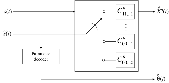
These ideas are formalized in Theorem III.2 below for i.i.d. vector sources $\{X_{i}\}$, $X_{i}\in\mathbb{R}^{d}$, where the common distribution of the $X_{i}$’s is a member of a given indexed class $\{P_{\theta}:\theta\in\Theta\}$ of absolutely continuous distributions, and the parameter space $\Theta$ is a bounded subset of $\mathbb{R}^{k}$. For simplicity we have set $m=n$, although other choices for the memory length are also possible. Before we state and prove the theorem, let us fix some useful results and notation. The following proposition generalizes Theorem 2 of Linder, Lugosi and Zeger [11] to i.i.d. vector sources and characterizes the rate at which the $n$th-order operational DRF converges to the Shannon DRF (the proof, which uses Csiszár’s generalized parametric representation of the DRF [23], as well as a combination of standard random coding arguments and large-deviation estimates, is an almost verbatim adaptation of the proof of Linder et al. to vector sources, and is presented for completeness in Appendix B):

The distance between two i.i.d. sources will be measured by the variational distance between their respective single-letter distributions [19, Ch. 5]:

$$d_{V}(P_{\theta},P_{\eta})\stackrel{{\scriptstyle\scriptscriptstyle\triangle}}{{=}}\sup_{B}|P_{\theta}(B)-P_{\eta}(B)|,\qquad\forall\theta,\eta\in\Theta$$

where the supremum is taken over all Borel subsets of $\mathbb{R}^{d}$. Also, given a sequence of real-valued random variables $V_{1},V_{2},\cdots$ and a sequence of nonnegative numbers $a_{1},a_{2},\cdots$, the notation $V_{n}=O(a_{n})$ a.s. means that there exist a constant $c>0$ and a nonnegative random variable $N\in\mathbb{Z}$ such that $V_{n}\leq ca_{n}$ for all $n\geq N$. Finally, both the statement and the proof of the theorem rely on certain notions from Vapnik–Chervonenkis theory; for the reader’s convenience, Appendix A contains a summary of the necessary definitions and results.

Proof: The theorem will be proved by construction of a two-stage code, where the first-stage encoder $\widetilde{f}:{\cal X}^{n}\rightarrow\widetilde{{\cal S}}$ is a cascade of the parameter estimator $\widetilde{\theta}:{\cal X}^{n}\rightarrow\Theta$ and the lossy parameter encoder $\widetilde{g}:\Theta\rightarrow\widetilde{{\cal S}}$. Estimation of the parameter vector $\theta$ at the decoder will be facilitated by the corresponding decoder $\widetilde{\psi}:\widetilde{{\cal S}}\rightarrow\Theta$.

Our parameter estimator will be based on the so-called minimum-distance density estimator [16, Sec. 5.5], originally developed by Devroye and Lugosi [17, 18] in the context of kernel density estimation. It is constructed as follows. Let $Z^{n}=(Z_{1},\cdots,Z_{n})$ be i.i.d. according to $P_{\theta}$ for some $\theta\in\Theta$. Given any $\eta\in\Theta$, let

$$\Delta_{\eta}(Z^{n})\stackrel{{\scriptstyle\scriptscriptstyle\triangle}}{{=}}\sup_{A\in{\cal A}_{\Theta}}\left|P_{\eta}(A)-P_{Z^{n}}(A)\right|,$$

where $P_{Z^{n}}$ is the empirical distribution of $Z^{n}$,

$$P_{Z^{n}}(B)\stackrel{{\scriptstyle\scriptscriptstyle\triangle}}{{=}}\frac{1}{n}\sum^{n}_{i=1}1_{\{Z_{i}\in B\}}$$

for any Borel set $B$. Define $\widetilde{\theta}(Z^{n})$ as any $\theta^{*}\in\Theta$ satisfying

$$\Delta_{\theta^{*}}(Z^{n})<\inf_{\eta\in\Theta}\Delta_{\eta}(Z^{n})+\frac{1}{n},$$

where the extra $1/n$ term has been added to ensure that at least one such $\theta^{*}$ exists. Then $P_{\widetilde{\theta}(Z^{n})}$ is called the minimum-distance estimate of $P_{\theta}$. Through an abuse of terminology, we shall also say that $\widetilde{\theta}$ is the minimum-distance estimate of $\theta$. The key property of the minimum-distance estimate [16, Thm. 5.13] is that

$$\int_{\cal X}|p_{\widetilde{\theta}(Z^{n})}(x)-p_{\theta}(x)|dx\leq 4\Delta_{\theta}(Z^{n})+\frac{3}{n}.$$

(3.7)

Since the variational distance between any two absolutely continuous distributions $P,Q$ on $\mathbb{R}^{d}$ is equal to one half of the $L_{1}$ distance between their respective densities $p,q$ [19, Thm. 5.1], i.e.,

$$d_{V}(P,Q)=\frac{1}{2}\int_{\mathbb{R}^{d}}|p(x)-q(x)|dx,$$

we can rewrite (3.7) as

$$d_{V}(P_{\theta},P_{\widetilde{\theta}(Z^{n})})\leq 2\Delta_{\theta}(Z^{n})+\frac{3}{2n}.$$

(3.8)

Since ${\cal A}_{\Theta}$ is a Vapnik–Chervonenkis class, Lemma A.2 in the Appendices asserts that

$$\operatorname{{\mathbb{E}}}_{\theta}[\Delta_{\theta}(Z^{n})]\leq c_{1}\sqrt{\frac{\log n}{n}},$$

(3.9)

where $c_{1}$ is a constant that depends only on the VC dimension of ${\cal A}_{\Theta}$. Taking expectations of both sides of (3.8) and applying (3.9), we get

$$\operatorname{{\mathbb{E}}}_{\theta}\left[d_{V}(P_{\theta},P_{\widetilde{\theta}(Z^{n})})\right]\leq 2c_{1}\sqrt{\frac{\log n}{n}}+\frac{3}{2n}.$$

(3.10)

Next, we construct the lossy encoder $\widetilde{g}$. Since $\Theta$ is bounded, it is contained in some hypercube $M$ of side $J$, where $J$ is some positive integer. Let ${\cal M}^{(n)}=\{M^{(n)}_{1},M^{(n)}_{2},\cdots,M^{(n)}_{K}\}$ be a partitioning of $M$ into nonoverlapping hypercubes of side $1/\lceil n^{1/2}\rceil$, so that $K\leq(Jn^{1/2})^{k}$. Represent each $M^{(n)}_{j}$ that intersects $\Theta$ by a unique fixed-length binary string $\widetilde{s}_{j}$, and let $\widetilde{{\cal S}}=\{\widetilde{s}_{j}\}$. Then if a given $\theta\in\Theta$ is contained in $M^{(n)}_{j}$, map it to $\widetilde{s}_{j}$, $\widetilde{g}(\theta)=\widetilde{s}_{j}$; this choice can be described by a string of no more than $k(\log n^{1/2}+\log J)$ bits. Finally, for each $M^{(n)}_{j}$ that intersects $\Theta$, choose a representative $\widehat{\theta}_{j}\in M^{(n)}_{j}\cap\Theta$ and define the corresponding $n$-block code $C^{n}_{\widetilde{s}_{j}}$ to be $C^{n}_{\widehat{\theta}_{j}}$. Thus, we can associate to $\widetilde{g}$ the decoder $\widetilde{\psi}:\widetilde{{\cal S}}\rightarrow\Theta$ via $\widetilde{\psi}(\widetilde{s}_{j})=\widehat{\theta}_{j}$.

Now let us describe and analyze the operation of the resulting two-stage $(n,n)$-block code $C^{n,n}$. In order to keep the notation simple, we shall suppress the discrete time variable $t$ and denote the current block $X^{n}(t)$ by $X^{n}$, while the preceding block $X^{n}(t-1)$ will be denoted by $Z^{n}$. The first-stage encoder $\widetilde{f}$ computes the minimum-distance estimate $\widetilde{\theta}=\widetilde{\theta}(Z^{n})$ and communicates its lossy binary description $\widetilde{s}=\widetilde{f}(Z^{n})\equiv\widetilde{g}(\widetilde{\theta}(Z^{n}))$ to the second-stage encoder. The second-stage encoder then encodes $X^{n}$ with the $n$-block code $C^{n}_{\widetilde{s}}\equiv C^{n}_{\widehat{\theta}}$, where $\widehat{\theta}=\widetilde{\psi}(\widetilde{s})$ is the quantized version of the minimum-distance estimate $\widetilde{\theta}$. The string transmitted to the decoder thus consists of two parts: the header $\widetilde{s}$, which specifies the second-stage code $C^{n}_{\widetilde{s}}$, and the body $s=f_{\widetilde{s}}(X^{n})$, which is the encoding of $X^{n}$ under $C^{n}_{\widetilde{s}}$. The decoder computes the reproduction $\widehat{X}^{n}=\phi_{\widetilde{s}}(s)$. Note, however, that the header $\widetilde{s}$ not only instructs the decoder how to decode the body $s$, but also contains a binary description of the quantized minimum-distance estimate of the active source, which can be recovered by means of the rule $\widehat{\theta}=\widetilde{\psi}(\widetilde{s})$.

In order to keep the notation simple, assume for now that $p=1$, i.e., the distortion function $\rho$ is a metric on ${\cal X}\cup\widehat{\cal X}$ with the bound $\rho_{\max}$; the case of general $p$ is similar. The rate of $C^{n,n}$ is clearly no more than

$$R+\frac{k(\log n^{1/2}+\log J)}{n}$$

bits per letter, which proves (3.4). The average-per letter distortion of $C^{n,n}$ on the source $P_{\theta}$ is, in accordance with (3.2), given by

$$D_{\theta}(C^{n,n})=\operatorname{{\mathbb{E}}}_{\theta}\left[D_{\theta}\left(C^{n}_{\widetilde{f}(Z^{n})}\right)\right],$$

where $C^{n}_{\widetilde{f}(Z^{n})}=C^{n}_{\widehat{\theta}}$ with $\widehat{\theta}=\widetilde{\psi}(\widetilde{f}(Z^{n}))$. Without loss of generality, we may assume that each $C^{n}_{\theta}$ is a nearest-neighbor quantizer, i.e.,

$$\rho(x^{n},C^{n}_{\theta}(x^{n}))=\min_{\widehat{x}^{n}\in\Gamma_{\theta}}\rho(x^{n},\widehat{x}^{n})$$

for all $x^{n}\in{\cal X}^{n}$, where $\Gamma_{\theta}$ is the codebook of $C^{n}_{\theta}$. Then we have the following chain of estimates:

	$\displaystyle D_{\theta}(C^{n}_{\widehat{\theta}})$	$\displaystyle\stackrel{{\scriptstyle\rm(a)}}{{\leq}}$	$\displaystyle D_{\widehat{\theta}}(C^{n}_{\widehat{\theta}})+2\rho_{\max}d_{V}(P_{\theta},P_{\widehat{\theta}})$
		$\displaystyle\stackrel{{\scriptstyle\rm(b)}}{{=}}$	$\displaystyle\widehat{D}^{n}_{\widehat{\theta}}(R)+2\rho_{\max}d_{V}(P_{\theta},P_{\widehat{\theta}})$
		$\displaystyle\stackrel{{\scriptstyle\rm(c)}}{{\leq}}$	$\displaystyle\widehat{D}^{n}_{\theta}(R)+4\rho_{\max}d_{V}(P_{\theta},P_{\widehat{\theta}})$
		$\displaystyle\stackrel{{\scriptstyle\rm(d)}}{{\leq}}$	$\displaystyle\widehat{D}^{n}_{\theta}(R)+4\rho_{\max}\left[d_{V}(P_{\theta},P_{\widetilde{\theta}})+d_{V}(P_{\widetilde{\theta}},P_{\widehat{\theta}})\right],$

where (a) and (c) follow from a basic quantizer mismatch estimate (Lemma C.1 in the Appendices), (b) follows from the assumed $n$th-order optimality of $C^{n}_{\widehat{\theta}}$ for $P_{\widehat{\theta}}$, while (d) is a routine application of the triangle inequality. Taking expectations, we get

$$D_{\theta}(C^{n,n})\leq\widehat{D}^{n}_{\theta}(R)+4\rho_{\max}\left\{\operatorname{{\mathbb{E}}}_{\theta}[d_{V}(P_{\theta},P_{\widetilde{\theta}})]+\operatorname{{\mathbb{E}}}_{\theta}[d_{V}(P_{\widetilde{\theta}},P_{\widehat{\theta}})]\right\}.$$

(3.11)

We now estimate separately each term in the curly brackets in (3.11). The first term can be bounded using the fact that $\widetilde{\theta}=\widetilde{\theta}(Z^{n})$ is a minimum-distance estimate of $\theta$, so by (3.10) we have

$$\operatorname{{\mathbb{E}}}_{\theta}[d_{V}(P_{\theta},P_{\widetilde{\theta}})]\leq 2c_{1}\sqrt{\frac{\log n}{n}}+\frac{3}{2n}.$$

(3.12)

The second term involves $\widetilde{\theta}$ and its quantized version $\widehat{\theta}$, which satisfy $\|\widetilde{\theta}-\widehat{\theta}\|\leq\sqrt{k/n}$, by construction of the parameter space quantizer $(\widetilde{g},\widetilde{\psi})$. By the uniform local Lipschitz property of the map $\theta\mapsto P_{\theta}$, there exist constants $r>0$ and $m>0$, such that

$$d_{V}(P_{\eta},P_{\widehat{\theta}})\leq m\|\eta-\widehat{\theta}\|$$

for all $\eta\in B_{r}(\widehat{\theta})$. If $\widetilde{\theta}\in B_{r}({\widehat{\theta}})$, this implies that $d_{V}(P_{\widetilde{\theta}},P_{\widehat{\theta}})\leq m\sqrt{k/n}$. Suppose, on the other hand, that $\widetilde{\theta}\not\in B_{r}({\widehat{\theta}})$. By assumption, $\|\widetilde{\theta}-\widehat{\theta}\|\geq r$. Therefore, since $d_{V}(\cdot,\cdot)$ is bounded from above by unity, we can write

$$d_{V}(P_{\widetilde{\theta}},P_{\widehat{\theta}})\leq\frac{1}{r}\|\widetilde{\theta}-\widehat{\theta}\|\leq\frac{1}{r}\sqrt{\frac{k}{n}}.$$

Let $b\stackrel{{\scriptstyle\scriptscriptstyle\triangle}}{{=}}\max(m,1/r)$. Then the above argument implies that

$$d_{V}(P_{\widetilde{\theta}},P_{\widehat{\theta}})\leq b\sqrt{\frac{k}{n}}$$

(3.13)

and consequently

$$\operatorname{{\mathbb{E}}}_{\theta}[d_{V}(P_{\widetilde{\theta}},P_{\widehat{\theta}})]\leq b\sqrt{\frac{k}{n}}.$$

(3.14)

Substituting the bounds (3.12) and (3.14) into (3.11) yields

$$D_{\theta}(C^{n,n})\leq\widehat{D}^{n}_{\theta}(R)+\rho_{\max}\left(8c_{1}\sqrt{\frac{\log n}{n}}+\frac{6}{n}+4b\sqrt{\frac{k}{n}}\right),$$

whence it follows that the $n$th-order redundancy $\delta^{n}_{\theta}(C^{n})=O(\sqrt{n^{-1}\log n})$ for every $\theta\in\Theta$. Then the decomposition

$$\delta_{\theta}(C^{n,n})=\delta^{n}_{\theta}(C^{n,n})+\widehat{D}^{n}_{\theta}(R)-D_{\theta}(R)$$

and Proposition III.1 imply that (3.5) holds for every $\theta\in\Theta$. The case of $p\neq 1$ is similar.

References

- [1] J. Rissanen, “Universal coding, information, prediction, and estimation,” IEEE Trans. Inform. Theory, vol. IT-30, no. 4, pp. 629–636, July 1984.
- [2] ——, “Stochastic complexity and modeling,” Ann. Statist., vol. 14, no. 3, pp. 1080–1100, September 1986.
- [3] ——, “Fisher information and stochastic complexity,” IEEE Trans. Inform. Theory, vol. 42, no. 1, pp. 40–47, January 1996.
- [4] A. Barron, J. Rissanen, and B. Yu, “Minimum description length principle in coding and modeling,” IEEE Trans. Inform. Theory, vol. 44, no. 6, pp. 2743–2760, October 1998.
- [5] P. D. Grünwald, The Minimum Description Length Principle. MIT Press, 2007.
- [6] T. M. Cover and J. A. Thomas, Elements of Information Theory. New York: Wiley, 1991.
- [7] G. Tao, Adaptive Control Design and Analysis. Hoboken: Wiley, 2003.
- [8] J. Ziv, “Coding of sources with unknown statistics – Part II: Distortion relative to a fidelity criterion,” IEEE Trans. Inform. Theory, vol. IT-18, no. 3, pp. 389–394, May 1972.
- [9] D. L. Neuhoff, R. M. Gray, and L. D. Davisson, “Fixed rate universal block source coding with a fidelity criterion,” IEEE Trans. Inform. Theory, vol. IT-21, no. 5, pp. 511–523, September 1975.
- [10] T. Linder, G. Lugosi, and K. Zeger, “Rates of convergence in the source coding theorem, in empirical quantizer design, and in universal lossy source coding,” IEEE Trans. Inform. Theory, vol. 40, no. 6, pp. 1728–1740, November 1994.
- [11] ——, “Fixed-rate universal lossy source coding coding and rates of convergence for memoryless sources,” IEEE Trans. Inform. Theory, vol. 41, no. 3, pp. 665–676, May 1995.
- [12] Z. Zhang and V. K. Wei, “An on-line universal lossy data compression algorithm via continuous codebook refinement — Part I: Basic results,” IEEE Trans. Inform. Theory, vol. 42, no. 3, pp. 803–821, May 1996.
- [13] P. A. Chou, M. Effros, and R. M. Gray, “A vector quantization approach to universal noiseless coding and quantization,” IEEE Trans. Inform. Theory, vol. 42, no. 4, pp. 1109–1138, July 1996.
- [14] R. F. Rice and J. R. Plaunt, “The Rice machine: television data compression,” Jet Propulsion Lab, Pasadena, CA, Tech. Rep. 900-408, September 1970.
- [15] ——, “Adaptive variable-length coding for efficient compression of spacecraft television data,” IEEE Trans. Commun., vol. COM-19, pp. 889–897, December 1971.
- [16] L. Devroye and L. Györfi, “Distribution and density estimation,” in Principles of Nonparametric Learning, L. Györfi, Ed. New York: Springer-Verlag, 2001.
- [17] L. Devroye and G. Lugosi, “A universally acceptable smoothing factor for kernel density estimation,” Ann. Statist., vol. 24, pp. 2499–2512, 1996.
- [18] ——, “Nonasymptotic universal smoothing factors, kernel complexity and Yatracos classes,” Ann. Statist., vol. 25, pp. 2626–2637, 1997.
- [19] ——, Combinatorial Methods in Density Estimation. New York: Springer-Verlag, 2001.
- [20] D. L. Neuhoff and R. K. Gilbert, “Causal source codes,” IEEE Trans. Inform. Theory, vol. IT-28, no. 5, pp. 701–713, September 1982.
- [21] R. M. Gray, D. L. Neuhoff, and J. K. Omura, “Process definitions of distortion-rate functions and source coding theorems,” IEEE Trans. Inform. Theory, vol. IT-21, no. 5, pp. 524–532, September 1975.
- [22] R. G. Gallager, Information Theory and Reliable Communication. New York: Wiley, 1968.
- [23] I. Csiszár, “On an extremum problem in information theory,” Stud. Sci. Math. Hung., vol. 9, pp. 57–70, 1974.
- [24] Y. G. Yatracos, “Rates of convergence of minimum distance estimates and Kolmogorov’s entropy,” Ann. Math. Statist., vol. 13, pp. 768–774, 1985.
- [25] I. Csiszár and J. Körner, Information Theory: Coding Theorems for Discrete Memoryless Sources. Budapest: Akadémiai Kiadó, 1981.
- [26] R. M. Gray, D. L. Neuhoff, and P. S. Shields, “A generalization of Ornstein’s distance with applications to information theory,” Ann. Probab., vol. 3, no. 2, pp. 315–328, 1975.
- [27] A. N. Kolmogorov and V. M. Tihomirov, “-entropy and -capacity of sets in function spaces,” in Amer. Math. Soc. Transl., ser. 2, 1961, vol. 17, pp. 277–364.
- [28] S. Amari and H. Nagaoka, Methods of Information Geometry. Providence: American Mathematical Society, 2000.
- [29] R. García-Muñoz and D. L. Neuhoff, “Strong universal source coding subject to a rate-distortion constraint,” IEEE Trans. Inform. Theory, vol. IT-28, no. 2, pp. 285–295, March 1982.
- [30] R. L. Dobrushin, “Unified methods for optimal quantization of messages,” in Problemy Kibernetiki, A. A. Lyapunov, Ed. Moscow: Nauka, 1970, vol. 22, pp. 107–156, in Russian.
- [31] D. J. Sakrison, “The rate distortion function for a class of sources,” Inform. Control, vol. 15, pp. 165–195, 1969.
- [32] ——, “Worst sources and robust codes for difference distortion measures,” IEEE Trans. Inform. Theory, vol. IT-21, no. 3, pp. 301–309, May 1975.
- [33] D. L. Neuhoff and R. García-Muñoz, “Robust source coding of weakly compact classes,” IEEE Trans. Inform. Theory, vol. IT-33, no. 4, pp. 522–530, July 1987.
- [34] H. W. Sorenson and D. L. Alspach, “Recursive Bayesian estimation using Gaussian sums,” Automatica, vol. 7, no. 4, pp. 465–479, July 1971.
- [35] A. R. Barron and C.-H. Sheu, “Approximation of density functions by sequences of exponential families,” Ann. Statist., vol. 19, no. 3, pp. 1347–1369, 1991.
- [36] H. Zhuang, Y. Huang, K. Palaniappan, and Y. Zhao, “Gaussian mixture density modeling, decomposition, and applications,” IEEE Trans. Image Processing, vol. 5, no. 9, pp. 1293–1302, September 1996.
- [37] M. A. T. Figueiredo and A. K. Jain, “Unsupervised learning of finite mixture models,” IEEE Trans. Pattern Anal. Machine Intelligence, vol. 24, no. 3, pp. 381–396, March 2002.
- [38] R. M. Gray, Entropy and Information Theory. New York: Springer-Verlag, 1990.
- [39] I. Kontoyiannis and J. Zhang, “Arbitrary source models and Bayesian codebooks in rate-distortion theory,” IEEE Trans. Inform. Theory, vol. 48, no. 8, pp. 2276–2290, August 2002.
- [40] E.-H. Yang and Z. Zhang, “The redundancy of source coding with a fidelity criterion – part II: Coding at a fixed rate level with unknown statistics,” IEEE Trans. Inform. Theory, vol. 47, no. 1, pp. 126–145, January 2002.
- [41] M. Madiman and I. Kontoyiannis, “Second-order properties of lossy likelihoods and the MLE/MDL dichotomy in lossy compression,” Brown University, APPTS Report No. 04-5, May 2004, available [Online] at http://www.dam.brown.edu/ptg/REPORTS/04-5.pdf.
- [42] M. Madiman, M. Harrison, and I. Kontoyiannis, “Minimum description length vs. maximum likelihood in lossy data compression,” in Proc. IEEE Int. Symp. on Information Theory, Chicago, 27 June – 2 July 2004, p. 461.
- [43] M. Raginsky, “Joint universal lossy coding and identification of stationary mixing sources with general alphabets,” IEEE Trans. Inform. Theory, 2006, submitted.
- [44] ——, “Joint universal lossy coding and identification of stationary mixing sources,” in Proc. IEEE Int. Symp. on Information Theory, Nice, France, June 2007, to appear.
- [45] P. Moulin and R. Koetter, “Data-hiding codes,” Proc. IEEE, vol. 93, no. 12, pp. 2085–2127, December 2005.
- [46] V. N. Vapnik and A. Y. Chervonenkis, “On the uniform convergence of relative frequencies of events to their probabilities,” Theory Probab. Appl., vol. 16, pp. 264–280, 1971.
- [47] N. Sauer, “On the density of families of sets,” J. Combin. Theory Ser. A, vol. 13, pp. 145–147, 1972.
- [48] R. M. Dudley, “Central limit theorems for empirical measures,” Ann. Probab., vol. 6, pp. 898–929, 1978.
- [49] W. Hoeffding, “Probability inequalities for sums of bounded random variables,” J. Amer. Statist. Soc., vol. 58, pp. 13–30, 1963.
- [50] T. Lindvall, Lectures on the Coupling Method. New York: Dover, 2002.