Various Solutions for the Firing Squad Synchronization Problem. Work partially supported by the grant “Metodi Formali ed Algoritmi per la Verifica di Sistemi Distribuiti”, Università degli Studi di Salerno. The first author is also supported by the grant GAČR, 201/04/1153.
Abstract
We present different classes of solutions to the Firing Squad Synchronization Problem on networks of different shapes. The nodes are finite state processors that work at unison discrete steps. The networks considered are the line, the ring and the square. For all of these models we have considered one and two-way communication modes and also constrained the quantity of information that adjacent processors can exchange each step. We are given a particular time expressed as a function of the number of nodes of the network, and present synchronization algorithms in time , , , . The solutions are presented as signals that are used as building blocks to compose new solutions for all times expressed by polynomials with nonnegative coefficients.
1 Introduction
The famous firing squad synchronization problem (FSSP), is an old problem posed by Myhill in 1957 (in print in [18]). In terms of Cellular Automata, we are given a line of identical cells (finite state machines) that work synchronously at discrete time steps, initially a distinguished cell (the so called general) starts computing while all others are in a quiescent state; at each time step any cell sends/receives to/from its neighbours some information about their state at the preceding time: the problem is to let all cells in the line enter the same state, called firing, for the first time and at the very same instant, the firing time.
In literature many solutions to the original problem and to some variations of it have been given. The early results all focused on the synchronization in minimal time: Minsky in [17] showed that a solution to the FSSP requires at least time, Waksman [22] and Balzer [1] gave the first solution in this minimal time and Mazoyer in [14] constructed a minimal time solution with the least number of states to date: six. In [1] it has also been shown that five states are always necessary for a solution.
A significant amount of papers have also dealt with some variations of the FSSP. These variations concerned both the geometry of the network and some computational constraints. In the following we briefly recall some of them. The FSSP has been studied on a (one-way) ring of processors [4, 11], on arrays of two and three-dimensions [21, 8]: in all these papers all the results focused on lower and upper bounds on the minimal time for the synchronization. In the very recent paper [9] the cells of the network are placed along a path in the two-dimensional array space, there a combinatorial problem (for which only exponential algorithms are known) is reduced to the existence of an optimal solution to the FSSP on this path. In [20] solutions for the Cayley graphs are given and in [19] a particular class of graphs is studied and for this class a solution in time or is given, where is the longest distance between the general and any other node (the radius) of the graph. Some constrained variants of the FSSP have concerned solutions on the interesting model of reversible CA (i.e., backward deterministic CA) [6] and CA with a number-conserving property (i.e., a state is a tuple of positive integers whose sum is constant during the computation) [7]. Other kinds of constraints which have been considered concern the amount of information exchanged between any pair of adjacent cells. In [15, 12] the network is a line of cells that can exchange only one bit, that is at each time step each cell sends/receives only one bit of information to/from the adjacent cells instead of its whole state. Finally let us recall the significant work of [2] where the FSSP is studied in a distributed setting (no global clock, but lock-step synchrony) with bounds on the number of faulty processors.
In this paper we consider the problem on various networks (line, ring, square), and for one and two-way communication modes, but with a new approach with respect to the past: we hypothesize we are given the firing time and we ask for a synchronization algorithm in this time. This is an interesting and challenging theoretical problem, which is also directly connected to the sequential composition of cellular automata. Given two cellular automata and computing respectively the functions and , the sequential composition of followed by is the cellular automaton obtained in the following way: first starts on a standard initial configuration and when it has done with its computation, starts using the final configuration of as initial configuration. The resulting automaton clearly computes . In order to compose the two automata it is necessary to synchronize all the cells that will be used by at the time computes .
Some of the results presented here are a revisiting and a generalization of some results of [11, 12, 13], anyway here we present a whole framework of signals that, informally speaking, is a set of cells that at a given time receive or send a particular state. We then define some basic signals (building blocks) and give some rules to combine them to obtain other new signals. This modular approach allows to design synchronizing algorithms in a very natural way also simplifying their understanding and descriptions. Moreover here we introduce also as a parameter the number of bits that can be simultaneously transmitted at each step. We study networks where at each step a cell can transmits to each of its neighbours at most bits, .
As said above the communication between adjacent cells can be in both directions or only in a direction. We thus consider either networks where a cell can exchange information with all its neighbours, or networks where for each cell, only a predetermined half of its neighbours can send information to it while the other half can only receive information from it (the information flow is unidirectional). In this second case, to guarantee the communication from a cell to all the others, we consider circularly shaped networks.
For all the considered networks we prove a lower bound on the time of a synchronization, then we prove its tightness by giving a matching synchronization. We obtain families of solutions to the considered variants of the FSSP in several times , where is the number of nodes of the network. The approach we follow is compositional: we first describe basic synchronizing algorithms and then we give general rules to compose synchronizations. The basic synchronizations in turn are obtained by composing elementary signals, which can be seen as fragments of cellular automata. A synchronization is thus a special signal obtained as a composition of many simpler signals. Compositional rules for both signals and synchronizations include parallel composition, sequential composition, and iterated composition. We also state some sufficient conditions to apply them. In the parallel composition we start many synchronizations or signals, all at the same time. In some cases, this composition can be used to select among different synchronizations depending on the number of cells in the network. Sequential composition appends a synchronization (or a signal) to the end of another signal, possibly with a constant time offset. This way we are able to construct a synchronization in time , for , if there exist synchronizations in time and . If we are given two synchronizations respectively in time and , the iterated composition consists of iterating times the synchronization in time , thus obtaining a new synchronization in time . Compositions of synchronizations are used to determine synchronizations in a “feasible” time expressed by any polynomial with nonnegative coefficients. Finally, we give a construction to “inherit” synchronizations on two-dimensional networks starting from synchronizations of the corresponding linear networks. We show that an array of cells can be seen as many lines of cells (each of them having as endpoints cells and ) and a given synchronization on a line can be executed simultaneously on all these lines. Thus we can synchronize an array in time , provided that there exists a synchronizing algorithm for a line of cells in time .
As building blocks for the compositional rules we give synchronizing algorithms in some common functions: , , and . To synchronize a line of cells in time we first design some basic signals and then we compose them to obtain an overall signal that starts from the leftmost cell and comes back to it in exactly time units; then a minimal time synchronization starts, synchronizing the cells in time . To obtain a synchronization in time of an array of cells we use the following approach: first synchronize a row in time then start a synchronization in time on all the columns such that .
It is worth noticing that the composition rules also apply to the general case of arrays. Thus all the synchronizations given for an array can be extended to an array, considering the time of the synchronization as a function of either or .
The remainder of this paper is organized as follows. In section 2 we give the definitions and introduce the notation we will use throughout the rest of the paper. In section 3 we give tight lower bounds on the time synchronization of -CA and solutions in minimal time. In section 4 the framework of the signals is presented formally. In section 5 some composition rules on synchronizations are defined. In sections 6 and 7 solutions in the given times , , and are given for the two-way and one-way communication models, respectively. As an application of the compositional rules to obtain new synchronizations, in section 8 we show how to obtain polynomial-time synchronizations on all the considered models. The conclusions are in section 9.
2 Preliminaries
In this section we give the basic definitions, introduce the models, which are generalizations of the well known model of cellular automata, and define our synchronization problem.
The models. A cellular automaton is an array of pair-wise connected finite-state machines, called cells (or sometimes processors), which operate synchronously at discrete time steps. We consider both one-dimensional and two-dimensional cellular automata. The connections between cells may be either one-way or two-way links. We consider a generalization of the known cellular automata since in our models the capacity of the channels, and then the communication complexity, may vary. We call a -link a channel being able to transfer bits simultaneously. All the cells are indistinguishable, anyway for descriptive reasons, in a one dimensional array of cells we will number them starting from 0; moreover cell 0 and cell are said boundary cells. Unless stated otherwise, in the following is the number of cells of the one-dimensional cellular automaton.
The behaviour of each cell is in accordance to finite state transition functions depending on both the state of the cell and the output given at the preceding step by some of the connected cells. We define a function which determines the neighbouring cells on which the transition function of a given cell depends. This function depends on whether the connections are one-way or two-way-links and may also vary for different cells (for example, in the case of the boundary cells). For a cellular automaton , we denote by the maximum length of , for .

A c-Line is a one dimensional cellular automaton where the connections are two-way -links and where the -th cell is connected to the ()-th and ()-th cells, for , the first cell is connected only to the second cell, and the last cell is connected only to the -th cell, thus , for , and (see Figure 1.a). A c-Ring is a one dimensional cellular automaton with two-way -links with a connection also between the first and the last cell (see Figure 1.c). Thus it has a circular shape and the length of is two, for every . Finally, a c-ORing is a one dimensional cellular automaton with one-way -links such that a connection exists also between the first and the last cells. The -ORing has also a circular shape with , for every , and . Thus : the -th cell receives only the output of the -th cell.
The two-dimensional case is a natural generalization of the already considered models. In a two-dimensional array of cells, the cells are numbered , starting from . In what follows is always the number of cells of the two-dimensional cellular automaton. Each cell , except for the boundary cells, is connected to cells (), (), () and (). In this case, if the connections are two-way links, then and, with one-way connections, .
We consider a c-Square, where the connections are two-way -links and each boundary cell is connected only to the neighbouring cells (see Figure 1.b). For example, in this network the cell is connected to the cells and , while a cell is connected to the cells and and . On the other hand, we can define the c-Square of Rings, where, similarly to the first and last cells in the c-Ring, the boundary cells are pair-wise connected, and c-Square of ORings where the connections are one-way -links (see Figure 1.d).
For simplicity, we do not consider the rectangular models, that is those obtained from arrays of cells. Many of the results in this paper can be extended to this case. Figure 2 summarizes the considered models with respect to both the paradigms non-circular vs. circular and two-way vs. one-way links. Observe that we do not consider the non-circular models with one-way links. These models are not meaningful in this context.
Non-circular Circular -way -ORing, -Square of ORings -way -Line, -Square -Ring, -Square of Rings
To define the behaviour of all the introduced models, we use the symbol referring to the set of states of a given cellular automaton . Different transition functions are defined for different communication complexities. If we consider -links then for the non-boundary cells the transition function is , where is the set of tuples with and . In the non-circular models we should also define transition functions for the boundary cells (recall these cells are connected to less adjacent cells). We omit the formal definitions of these functions since they are quite standard and can be easily obtained by the definition for the non-boundary cells. The behaviour of a cell can be described as follows. Let , if a cell is in the state and receives from the cells in , then it enters the state and sends the words . (Note that this definition is symmetric: the number of words that each cell sends coincides with the number of received words.)
Note that in the standard definition of cellular automaton each cell can send to its neighbouring cells just its state. Therefore, in this paper, whenever we consider a model with link capacity such that , we will omit the index (that is, we will just speak about a Line, Square, etc., instead of a -Line, -Square, etc.). Some of the results given in this paper hold for all the models, thus we will speak about a to mean any of the models above with link capacity .
A configuration of a one dimensional cellular automaton with -links is a mapping . At time , a configuration gives, for each cell , the state entered and the words of bits sent at this time. A starting configuration is a configuration at time . In the following we often write “” to denote a cellular automaton starting on a configuration . We consider the time-unrolling of , that is a time -space array. A pair in this array, with and , is called a site, and denotes the cell at time . The state of the cell at time is denoted by and the words of bits sent to the neighbours are denoted by and . Sometimes, to avoid ambiguities, we will use , and to denote the state or the words of bits sent by a cell at time in a fixed cellular automaton . A site is said to be active if either it changes its states at the next step, or sends/receives a words different from 0, that is when one of the following conditions holds:
- •
,
- •
either or ,
- •
there is such that either or .
In the two-dimensional cases a configuration is defined in a natural way and the time-unrolling consists of triple , with and , denoting the cell at time . The state of the cell at time is denoted by .
The problem. Here we introduce a synchronization problem which generalizes the so called Firing Squad Synchronization Problem (FSSP). Among the states of the considered cellular automaton, there are three distinguished states: the General state, the Latent state, and the Firing state. The state , also said quiescent as well, has the property that if a cell in state receives all words 0 from its neighbours it remains in the same state and sends the word 0 to its neighbours. A standard configuration is a configuration where the cell (respectively cell () in the two-dimensional case) is in state and sends a word different from 0 to each neighbour and all the other cells are in state and send the word 0.
A synchronization in time is a cellular automaton such that, starting from a standard configuration, all cells enter state at time for the first time. We will speak about a synchronization of a -Line, -Square, etc. when the cellular automaton is a -Line, a -Square, etc. Moreover, a cellular automaton which provides a synchronization in time is also called a solution in time of the FSSP, or simply a solution.
We introduce now two variations of the problem whose solutions are sometimes useful to synchronize CA. A Two-End synchronization in time is a Line such that at time all cells enter for the first time the state , starting from a configuration which differs from the standard one because both the cell and the cell are in the state . A Four-End synchronization in time is a Square such that at time all cells enter for the first time the state , starting from a configuration having the cells , , , in the state and the other cells in the Latent state.
It is simple to see that the synchronizations of cellular automata with different communication complexity are not unrelated problems. Actually, a synchronization of a -CA can be seen as a synchronization of a -CA for every . In particular we will often use the following propositions:
Proposition 1
If there is a synchronization of a in time , then there exists a synchronization of a in time , for any .
3 Minimal Time Solutions
In this section we give tight lower bounds on the time of synchronizations of and present the algorithms for the synchronization in minimal time.
3.1 Lower Bounds on the Time of the Synchronizations
A synchronization of a -Line requires at least time . Intuitively, this is the minimal time for the first cell to wake up all the other cells and to get back the message that all the cells have been awakened. Recall that in a starting configuration each cell, except the first, is in a Latent state and the cell can leave the Latent state not before than time . Thus all the cells are awake at time , and the first cell gets this information back at time .
As regards the two-dimensional cellular automaton, Shinahr [21] has shown that the minimum time for synchronizing a rectangular array of cells is , but this time reduces to in the case of a Square. The following lemma summarizes these results.
Lemma 1
Every synchronization of a -Line or a -Square has time greater than or equal to .
The minimum time to synchronize a Ring or Square of Rings is at least, as above, the time required by the first cell to send a message to all the other cells and to get the information back.
Lemma 2
Every synchronization of a -Ring or a -Square of Rings has time greater than or equal to .
In the next Lemma we show that time is necessary to synchronize a -ORing and in Lemma 4 we show that the minimal time is for a -Square of ORings.
Lemma 3
Every synchronization of a -ORing has time greater than or equal to .
Proof : Assume by contradiction that there exists a synchronization within time of a ORing (say ) and let be an ORing which differs from just for the size: has cells instead of . Since for all , and , then and for all and . Observe that the state of the cell at time , for , depends on the states at time of the following cells: the cells and , when , the states of the cells , and , when , and in General on the states of the cells for . As a consequence, for . If , then at time the cell of both and will enter the state . Anyway the cell of at time is still in the state , thus we have a contradiction.
Lemma 4
Every synchronization of -Square of ORings has time greater than or equal to .
Proof : Assume by contradiction that there exists a synchronization in time of a Square of ORings and let and be a Square of ORings which differs from for the number of cells: instead of . Since for all and , and , then for all and . Furthermore, for both and the state of cell at time is for all cells such that . The state of the cell at time , for , depends on the states at time of the cells , for . As a consequence, at time the cell of both and will enter the state . Anyway since the cell of at time is still in the state , we have a contradiction.
3.2 Synchronization in Minimal Time for Two-way Communication Networks
In this subsection we present the minimal time algorithms for the synchronization of the models whose connections are two-way links. The Proposition 1 allows us to prove the statements only for the case .
Waksman in [22] gave the first solution to the problem of synchronizing a Line in the minimal time , and Mazoyer, in [15] showed that a minimal time synchronization exists for a -Line. Moreover, Shinahr [21] has shown the minimal time solution for a Square. In [10], the approach by Shinahr is combined with the solution by Mazoyer to obtain a minimal time synchronization of a -Square.
Lemma 5
For every link capacity , there is a synchronization of a -Line and of a -Square in time .
The above synchronizations can be used to obtain a Two-End synchronization of a Line and a Four-End synchronization of a Square in time as shown in the following lemma.
Lemma 6
There are a Two-End synchronization of a Line in time and a Four-End synchronization of a Square in time .
Proof : The Two-End synchronization in time can be obtained by considering a line as split in two halves and synchronizing each of them separately by a minimal time solution. This can be implemented by just starting a minimal time solution from both ends. In fact, each cell can determine its membership to a sub-line at the time it moves from the Latent state: this happens by a communication received from its left neighbour (membership to the left half-line), or from its right neighbour (membership to the right half-line). Note that, in case is odd, the central cell belongs to both half-lines, while when is even, the central cells start acting as the last cells of their half-lines with time unit of delay (at the time they receive a communication from the other half-line). Therefore, in both cases the Line is synchronized in time .
Consider now a Square. We rearrange it in concentric frames, where the -th inner frame is constituted by the four lines , , and , see Figure 3. Suppose now that the cells and are all in the same General state. The four lines of the first frame can all synchronize in time using the above result on the Two-End synchronization of a Line; during such synchronizations, after the first two steps, the four cells , , and all enter a General state and thus the four lines of the second frame can synchronize in time . Iterating this argument, the -th frame synchronizes in time , . As this synchronization starts at time , then the overall time to synchronize the processors is still .
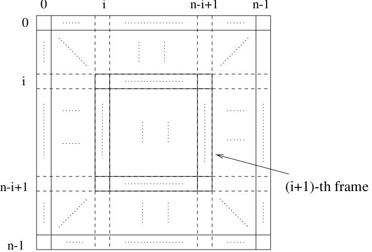
The synchronizations sketched in the above proof do not work when the link capacity is . The main reason is that synchronizations of -CA critically use the parity of the time a bit is received to distinguish between different messages. In particular, each cell expects an even time delay between the message sent by the General to wake up all cells and the reply sent by the last cell in the Line (in a minimal time solution the last cell replies as soon as it gets awakened). In the schema sketched in the proof of Lemma 6 for the Two-End synchronization of a Line, when is even, the central cells delay the response of time unit. Therefore, the reply message would be misunderstood by all the other cells, unless we delay it by another time unit. This is the idea exploited in the solution given in [10]. Therefore, we have the following lemma.
Lemma 7
There are a Two-End synchronization of a Line in time and a Four-End synchronization of a Square in time .
Note that the minimal time synchronization of a -Line by Mazoyer [15], can be modified to work for a -Line without relying on the parity of delays to recognize messages (we simply use the second bit to do that). Thus, it is easy to verify that the schema sketched in the proof of Lemma 6 can be adapted to work for a -CA using techniques similar to that used in [10] for the -CA. Therefore, the following lemma holds.
Lemma 8
For every link capacity , there are a Two-End synchronization of a Line in time and a Four-End synchronization of a Square in time .
The following lemma states that the lower bounds given in the previous section for -Ring and -Square of Rings are tight for . Note that, for the Ring, a similar, but not correct result, can be found in [4].
Lemma 9
For every link capacity , there is a synchronization of a -Ring and of a -Square of Rings in time . Moreover, there is a synchronization of a -Ring and of a -Square of Rings in time .
Proof : A -Ring can simulate a Two-End synchronization of a -Line of cells, so obtaining a synchronization in time . Actually, the cell can act as both the boundary cells of the -Line.
A synchronization of a -Square of Rings in time can be obtained by looking at this Square as split in three parts: the first row, the first column and the remaining of the array, that is a subarray of cells. As we have just noticed, the first row and the first column can be synchronized in time . During these synchronizations (in the first two steps) the cells , , , can enter a new state acting as a General state of a Four-End synchronization of a Square of cells. Using Lemmas 8 and 7 and considering that this last synchronization starts with a two step delay, we get the stated results.
We can give now the main results of the section.
Theorem 1
- •
For every link capacity , there is a synchronization of a -Line and of a -Square in time ; moreover, every synchronization of a -Line or a -Square has time greater than or equal to .
- •
For every link capacity , there is a synchronization of a -Ring and of a -Square of Rings in time , and there is a synchronization of a -Ring and of a -Square of Rings in time ; moreover, for every link capacity , every synchronization of a -Ring or a -Square of Rings has time greater than or equal to .
We observe that there is a gap between the shown lower and upper bounds for the synchronization of a -Ring and a -Square of Rings only for when is odd.
3.3 Synchronization in Minimal Time for One-way Communication Networks
The following two lemmas state that the lower bounds given in the previous section for the models using one-way links are tight.
Lemma 10
There is a synchronization of a ORing in time .
Proof : Using standard techniques, a computation of a Line of processors in time can be executed by an ORing in time , provided that the initial configuration of can be reached in one step from the initial configuration of . We informally use an induction on the number of steps. Let and and assume that . (To be more precise, since the cell of has to simulate the cell of , then when or when the state of the cell of encodes a state of and the information that the simulated cell is the leftmost or the rightmost in the line). Now the cell of at the next step needs the states of cells and at the time . Cell of passes its own state to the cell and this in turn forwards along with its state to the right neighbouring cell, the cell . This last cell can simulate the behaviour of the cell of at the step . Thus . The overall simulation takes thus a multiplicative delay factor of two.
Let us consider now a Two-End synchronization of a Line. It takes time and a synchronization of an ORing in time can be obtained with the above simulation. Actually, in the first step it lets the second cell enter a General state, so that the state of the cell after the first step is equal to the state of the cell in the starting configuration of .
Lemma 11
There is a synchronization of a Square of ORings in time .
Proof : We will first give an easier to describe solution which takes time and then we show how to save one time unit.
Using standard techniques (as in the previous proof), any computation of a Square in time can be executed by a Square of ORings in time in the following way. We informally use an induction on the number of steps. Assume that the cell in the third configuration of contains the state that the cell has in the first configuration of and that cell of at the time has the state that cell of has at the time . Actually, when the cell is a border cell, i.e. when either or , also this information is stored in the state of the cell of . Now the cell of at the -th step computes the new state from its own state and the states of cells , , and at time . Within three steps the cell of can collect the states that at time are in the cells , , , and . Namely:
- 1.
at step , cell of stores the two states of cells and ;
- 2.
at step the states are passed to cells and (note that in the previous step the state of cell at time has been passed to these cells);
- 3.
at step , cell simulates cell of at step .
So the state of the cell of at time contains the state that the cell of has at time . The overall simulation takes thus a multiplicative delay factor of three.
Let now be a Four-End synchronization as in Lemma 6. Recall that in this automaton, the Square is seen as organized in concentric frames (see Figure 3) which are synchronized at the same time . We can get a Square of ORings which in the first two steps reaches a configuration such that the states of all the cells and contain the General state (recall that the states of the cells and in the starting configuration of the solution are all the General state). Then simulates the solution within time .
Now let us briefly explain how can be modified to save one step, thus reaching time . The first steps (and thus the first configurations) remain unmodified. Let us observe what follows:
- 1.
Each cell of in the configuration participates for the synchronization of the frame which it belongs to; actually each cell participates either only for a row line or only for a column line of the frame except for the four corner cells of the frame which participate for both the lines. The same holds also for in the configurations (due to the mapping between the cells of the configuration of and those of configuration of ).
- 2.
At time in , , a cell is aware of the states at time of the following cells:
- a)
, , and ;
- b)
, , and .
- a)
Thus at step , the cell can correctly simulate either cell or cell of at step , hence entering the Firing state. In particular the cell simulates the former if participates to the synchronization for a row line, or simulates the latter, if participates to the simulation for a column line (note that at least one of these conditions must hold). Then, there is a Square of ORings inch is a synchronization in time .
We can give now the main results of the section.
Theorem 2
- •
There is a synchronization of an ORing in time and every synchronization of an ORing has time greater than or equal to .
- •
There is a synchronization of a Square of ORings in time and every synchronization of a Square of ORings has time greater than or equal to .
4 Signals
The framework of a signal has been introduced in [12] to simplify the design of a -Line. This innovative definition provides a way to modularize the design of solutions. Informally speaking, a signal is a particular set of cells that at a given time receives/sends a word different from from/to the adjacent cells. In other words a signal describes the information flow in the space-time unrolling of a cellular automaton, allowing a modular description of the synchronization process, that is starting from basic signals we combine different signals to obtain new ones to describe in a more natural way the synchronizing algorithms. (Let us note that also in [3] and [16] the signals were used, anyway there the intended meaning was different). The scheme used to present some synchronization algorithms in time for a -Line of processors is the following: some signals are designed and composed to obtain an overall signal that starts from the leftmost processor and comes back to it in exactly time units; then a minimal time synchronization starts, thus synchronizing the processors in time .
We consider the time unrolling of a -Line a configuration . Define the time is active and is active. Consider the set of all cells such that there exists at least an active site of , for such cells the set of sites is called the rear of and the set of sites is the front of . Moreover we say that is tailed if there exists a subset of , called tail such that for all , if and only if belongs to the front of . The states in are called tail states. In words, a tail state appears for the first time (in the time unrolling of ) on the front of .
Two active sites are consecutive if
and .
A simple signal of is a subset of temporally
consecutive sites with the property that
if is tailed, then belongs to
.
The union of a finite number of simple signals of a given
is called signal of .
A graphical representation of a simple signal
is obtained by drawing a straight line between:
(i) every pair of sites and and
(ii) every pair of sites and (resp.
) if (resp. ).
A graphical representation of a signal is obtained by the
graphical representation of its simple signals.
The length of a signal is
where and .
Sometimes, in the rest of the paper we refer to a signal without
specifying an automata and a starting configuration.
The following examples show two signals: Max and Mark. The former is the “fastest” signal (it touches one new cell each time unit), while the latter will be used to check the occurrence of an event (generally a signal crossing a given cell) thus if it is this case, triggering a new signal (see Figure 4).
Example 1
Let and be the set containing the sites if , or sites otherwise, for . This set is a simple signal, with length , of a tailed -Line that starts from a configuration having the states of cells and different from all the others.
Example 2
Given a positive constant , the signal is used to mark the cell . The length of the signal Mark is (see Figure 5). It can be easily seen that Mark is a signal of a tailed -Line.

4.1 Composition of Signals
Signals can be composed in order to obtain new ones. Given two signals and , we define the concatenation as the signal obtained by starting at time and at time , that is is delayed time steps. More formally, . In the concatenation of signals the following property is crucial. We say that a -Line on can follow a tailed -Line on if there exists a function defined over and such that if . When this property holds it is possible to switch from the front of to .
The following lemma recalls some sufficient conditions for the existence of a tailed -Line for a signal .
Lemma 12
Let and be signals of the tailed -Lines and , respectively. The signal is a signal of a tailed -Line if the following conditions hold:
- 1.
can follow ;
- 2.
if a site belongs to the front of and belongs to the rear of , then ;
- 3.
if sites and belong to the rear of then in .
Proof : Let be a site of a -Line such that is the in and belongs to the rear of . Define as . By the above property , this constant is well defined, and by the above property , it is greater than . A tailed -Line for , can be obtained in the following way. At the beginning behaves as . On the states from , counts up to and then enter the corresponding state of . We recall that this step is well defined since is a positive constant and the above property holds. At this point behaves as . Clearly, is tailed and is a signal of . Notice that if there are cells corresponding to active sites of which do not correspond to active sites of , from the above properties we have that in both configurations and they correspond to quiescent states.
4.2 Non trivial signals
We introduce here two non trivial signals of a -Line that will be used to get the main synchronization solutions of the section. The first has a quadratic length and the second has an exponential length in the number of cells. In particular from Proposition 1 it is sufficient to consider only the case (which is also the most difficult). For technical reasons in this section (and also in section 6 we will number the first cell as cell number (instead of as said in the preliminaries).
The signal Quad. Given a positive constant , is a signal of a -Line which is described as follows:
- •
initially the cell sends a bit to the right; then if it receives a bit from the right, it sends with a delay of one step (except for the first time, when there is no waiting), a bit back to the right; the cell eventually halts when it receives two consecutive bits ;
- •
for , the cell sends a bit to the left when it receives for the first time a bit from the left; then, if the cell receives again a bit from an adjacent cell, it sends a bit to the other adjacent cell;
- •
the cell sends two consecutive bits to the left when it receives a bit from the left.

Notice that the designed -Line can be tailed as well: in fact the cells from to can enter a tail state when they receive two consecutive bits . The length of the Quad signal is .
Let us note now that for the implementation of this signal the cell needs to be distinguished. In what follows we will use only in theorem 4 and in theorem 3, thus we only need to distinguish cells and : this can be done by and , for . For smaller much easier and ad hoc algorithms can be given (see Figure 5).
The signal Exp. Given two positive constants and , we will define the signal .
An idle cell is a cell which never sends a bit unless it receives a bit from the left and in this case it sends two consecutive bits to the left.
Initially the only idle cell is the cell . is a signal of a -Line which is described as follows:
- •
first cell sends a bit to the right; then, whenever cell receives a bit from the right, it immediately replies sending back a bit ; finally, if cell receives two consecutive bits from the right, then it changes into an idle cell;
- •
for , we distinguish two cases:
- –
if the bit is received from the left then it alternates the following two behaviours:
- 1.
it sends a bit back to the left; call these peak cells (though this is a property of the state entered by this cell.)
- 2.
it sends a bit to the right;
each peak cell starts counting from to , for . When has been just counted, if the peak cell receives a bit from the left at the next time unit, then it is the -th cell in the line and is marked (see below for an explanation). This way it can be distinguished later.
- 1.
- –
if a bit is received from the right, then it sends a bit to the left. If at the next time unit cell receives another bit from its right neighbour, then two other sub cases need to be considered:
-
if then the cell switches into an idle cell;
-
else, for , the cell sends two consecutive bits to the left. (Note that when this case occurs, cells have already been marked by step above.)
-
- –
From the algorithm we have just described, a proof by induction on can be given to show how a peak cell can be marked, in fact the following property holds: the length of the interval from the instant cell is a peak cell for the first time and the instant it becomes a peak cell for the second time is (see Figure 6 where , cell is marked at time and cell is marked at time ).

To implement a tailed -Line for initially the cell must be distinguished. In what follows we will use the signals and : the cells and can be distinguished by using and , for . Observe also that the cells from to can enter a tail state after they received two consecutive bits . The length of is (see Figure 6). In a very similar way we can define the signal of length (see Figure 7).

5 Composition of synchronizations
The design of synchronizations in times which are not minimal may not be obvious. A compositional approach to achieve this task is thus very useful. In this section we discuss several ways to combine two or more synchronizations of the models of networks we consider. We start with a parallel composition, then we study a sequential and an iterated compositions.
In the following, if is a synchronization of a -CA then , and denote the General, Latent and Firing states of and respectively, denote respectively the set of states and the transition function. We use the cross product of automata as a mean to combine -CA. Given a -Line and a -Line , we denote as the -Line defined as the standard cross product of and . Notice that in the construction we keep distinct the communication links of the two lines and thus allows to run in parallel synchronizations of a -Line along with synchronizations of a -Line. This construction is extended to all the other models we consider in an obvious way. We slightly modify the cross product construction to design a synchronization that selects among two different synchronizations according to a given condition . Examples of such conditions are the parity of the number of processors and the fastest/slowest synchronization. We define a selecting -Line in time as a -Line whose state set contains two disjoint subsets and , called the selection subsets, such that starting from a standard configuration its configuration at any time only contains either states from or states from . This definition is extended to all the other models we consider in an obvious way. The following lemma shows how to design a -CA that selects between two given synchronizations according to a condition on the number of cells. Clearly by iterating this construction, a selection among more than two synchronizations can be obtained.
Lemma 13
For , let be a synchronization on a -CA in time , and be a selecting -CA in time with selection subsets and . Then there exists a synchronization on a -CA in time such that , moreover if any configuration of at time contains only states from then , otherwise .
Proof : Let be the -CA obtained by modifying in the following way: for if a cell is entering and the selecting automaton is in a state from then it enters the firing state of . Clearly if starts on a configuration which is composed of triples of corresponding states of the standard configurations for , and , then synchronizes in the claimed time.
As applications of the above lemma we show two examples. In the first example we face with the problem of obtaining a synchronization which synchronizes at the maximum or at the minimum time between two synchronizations. We first define a selecting CA performing the test , then we show that this selecting CA can be used to obtain a synchronization in either the maximum or the minimum time between two synchronizations. In the second example a particular behaviour is selected depending on the result of a comparison between the number of processors and a constant .
Example 3
For denote by a synchronization in time . We define a selecting CA for the condition in time . The CA is mainly the cross product of and with the modification that once a synchronization enters the firing state, loops on this state. Thus we pick and . Thus by Lemma 13 we have a synchronization in time , if , and , otherwise. Thus a synchronization in the minimum time between and is obtained. If we pick instead and , then a synchronization in the maximum time between and is obtained.
Example 4
We describe a selecting CA performing the test , for a given positive integer . Let such that and are the General and Latent states respectively, and and . In the linear models the transition function can be informally described as follows. For the two-dimensional models can be described in an analogous way. In the first step cells and enter states and respectively; next, each cell in the Latent state enters the state if its adjacent cell on the left is in a state for , while it enters the state if this neighbour is in the state ; if each cell is in a state for some thus is propagated up to cell (this takes just a step in a ORing and steps in a Line since this is the case if cell is in a for ). When a processor enters the state or the state all the other processors are forced to enter the same state within a time . Obviously, is a selecting CA in time min.
Note that the selecting CA from the Example 4 can be used for any pair of synchronizations, as the time of the selecting CA is not larger than the time of any synchronization.
In the next two lemmas we show how to compose two synchronizations in time and respectively, to obtain synchronizations in time , for a given constant , and in time .
Lemma 14
If and are two synchronizations on a -CA respectively in time and , then there exists a synchronization on a -CA in time for .
Proof : We define a synchronization such that behaves as from time up to time , then at time it switches to . Thus is a synchronization in time . Furthermore, given a synchronization in time and with Firing state , a synchronization in time can be obtained from by adding the states and the transition rules from into for , and picking as the Firing state of the resulting synchronization.
Lemma 15
If and are two synchronizations on a -CA respectively in time and , then there exists a synchronization on a -CA in time .
Proof : We prove the above result for a -Line. The proof is similar ofr all the other models. We define a synchronization consisting of an Iterative phase of length which is executed times. The set of states of is , the General state is , the Latent state is and the Firing state is . In the Iterative phase, the synchronization modifies the first component of its state according to the transition functions of , until this component is . At the end of this phase executes a transition step modifying the second component of the state according to the transition functions of . The bits sent according to transition function of are saved in the last two components of each state according to the order left, right. Moreover, in this same step, replaces with either or (depending on whether the cell is the one triggering in the initial configuration the firing signal of ) in the first component. So the Iterative phase can start again, until the Firing state is entered by all the cells. So, the synchronization is iterated exactly times and takes time .
Finally we show a construction that allows to obtain synchronizations on a -Square in time provided that there exists a synchronization of on a -Line in time .
Lemma 16
Given a synchronization on a -Line in time , there exists a synchronization on a -Square in time .
Proof : An array can be seen as many lines of cells, each of them having as endpoints cells and . Each of these lines corresponds to a “path” from cell to cell going through exactly other cells. Each cell of these paths has as left neighbour either cell or cell and as right neighbour either cell or cell .
Notice that a cell is the -th cell from the left in all the lines it belongs to. This property allows us to execute simultaneously on all these lines a synchronization in time . Since the length of each line is , we have a synchronization of -Square in time .
6 Two-way communication Networks
In this section we compose the signals presented in the previous section to obtain solutions in time , , and on a -Line and on a -Square. Clearly these give as a corollary solutions in the same time for the -Line and -Square and for the circular -Ring and -Square of Rings.
For technical reasons we start numbering cells from (instead of ).
Theorem 3
There is a synchronization of a -Line in time .
Proof : The solution is divided into two phases. The first phase consists of and has length as is delayed one time step, see Figure 5. By Lemma 12, this phase is a signal of a tailed -Line starting from a standard configuration. Hence cell has entered a tailed state, say and considering this as the general state, a minimal time solution on a line is started, one step later: this is the second phase. Together the two phases give a solution to the FSSP in time .
Theorem 4
There is a synchronization of a -Square in time .
Proof : The algorithm is the following: first a signal is started on the first row, the length of this signal is since is delayed one time step. This is a signal of a tailed -Line starting from a standard configuration (see Lemma 12). Thus after time units the cell enters a tail state, say . Considering as the General state, a minimal time synchronization on a linear array of cells is executed on the first row and this takes other time units. Once the Firing state is reached, we use as the General state of a minimal time synchronization that this time runs on each column, thus taking another time units, which adds up to a total time of .
Theorem 5
There is a synchronization of a -Line in time .
Proof : The solution is divided into two phases. The first phase consists of and has length see Figure 6. By Lemma 12, this phase is a signal of a tailed -Line starting from a standard configuration. Hence cell has entered a tailed state, say and considering this as the general state, a minimal time solution on a line is started: this is the second phase. Together the two phases give a solution to the FSSP in time .
Theorem 6
There is a synchronization of a -Square in time .
Proof : First a signal is started on the first row, see Figure 6. After time units the cell enters a tail state, say . This is a signal of a tailed -Line starting from a standard configuration (see Lemma 12). Now the cell enters a state and a minimal time synchronization on the first row is accomplished, using as the General state, thus taking other time units. Once the Firing state is reached, each cell of the first row enters a state , and launches the signals and on each column, using as the General state. This takes another time units, which sums up to time . Finally, a minimal time synchronization on each column is accomplished, thus reaching time .
The proof of the existence of a synchronization of a -Line in time and in time is quite involved and long, see [12]. Here we recall the synchronization for the -Square.
Theorem 7
There is a synchronization of a -Square in time and in time .
Proof : The algorithms resemble those used to synchronize a line of cells at the same times of [12]. Therefore here we only outline the main idea. For the synchronization in time , we use a signal to synchronize the first row in time and then we apply a synchronization to each column in time (just a minimal time synchronization for a linear array with one more time unit).
Let us informally describe the synchronization of the first row. Initially the cells numbered ,, and are marked: this can be easily accomplished in time . This way the row can be seen as split in two halves and for each half a symmetric computation is done, therefore we will describe only the left half. A phase is iterated times: each iteration starts at time , , and has length . During the -th iteration, the test , is performed in the following way: a signal of length on the linear array consisting of the first cells and a signal Max of length , which is composed of Max() and Max(), are performed (see Figure 8). We compose the two signals to give Max a higher priority, thus if the exponential signal reaches a cell after the Max signal, it is aborted. In this case the Max signal finishes earlier than or at the same time as the exponential signal, and this means that and thus this is the last iteration. Otherwise (that is Max finishes later) cell is marked and a new iteration starts (see Figure 8). Omitting minor details, at the end of the last iteration all cells are forced in tail states, so determining a standard configuration for a synchronization of a linear array of cells in time . The synchronization in time can be obtained in a very similar way by considering a quadratic signal, instead of an exponential one, to synchronize the first row in time .

Corollary 1
There are synchronizations of a -Line, -Square and a -Ring, , in time , , and in time .
7 One-Way Communication Networks
In this section we give synchronization algorithms for the circular networks, ORings and Square of ORings, in time , , and . The algorithms in time is obtained by converting a solution for a CA. As in the previous section for technical reasons, we start numbering cells from (instead of ).
The following theorem gives the solution in time .
Theorem 8
There is a synchronization of a ORing and of Square of ORings in time .
Proof : First consider the ORing. Assume , the case can be dealt with a simple ad hoc strategy and we omit it (Lemma 13 can be used with the test to select the behaviour, see Example 4). The algorithm is very intuitive, thus we will not give the details of the signals.
The solution is divided into two phases: the Counting and the Synchronization phases. The Counting phase has length and can be seen as constituted by iterations of a sub-phase of steps. This sub-phase is simply a Max signal going all along the ring, from the first cell to the last. In the first iteration the cell number is marked with a marker and at each successive iteration is moved one cell to the right, so is moved to the first cell when iterations have been executed, that is at time . This phase is a signal of a tailed -Line starting from a standard configuration (see Lemma 12). The Synchronization phase consists of a minimal time solution (in time ) on a ring and can start exactly at time and the total solution has thus length .
Now let us consider the Square of ORings. Here assume and, as before, Lemma 13 is used to select the behaviour. The solution in time is easily obtained through the following two steps:
- •
the first row is synchronized in time with a minimal time solution on a ring;
- •
a solution in time is applied to each column.
The solution in time is easily obtained from a solution in time on a ring and modifying the first iteration of the Counting phase in order to mark the cell (instead of cell ). In this way the Counting phase is constituted by iterations of the sub-phase, thus saving steps.
Now we show how to obtain a solution in time . Let us recall that by Lemma 5 there is a two-end synchronization of a -Line in time . Notice that it is easy to modify this algorithm in such a way that in the -th configuration the processor , for a given , is in a particular state which is different from all other states entered by the any processor (actually this is a signal of type Mark). A similar result can be easily obtained for the ORing as well.
Lemma 17
There is a synchronization of a ORing in time such that in the configuration the processor , for a given is in a particular state which is different from the state of any other processor.
Now we can give the synchronization in time .
Theorem 9
There is a solution of an ORing and of a Square of ORings in time .
Proof : First consider the ORing. Let us assume for the moment . The solution is divided in three phases: the Initialization, the Iterative and the Synchronization phases. The Iterative phase is executed if , otherwise it is skipped. Informally speaking the whole solution is described as follows.
In the Initialization phase the cell is marked with a particular state, call it marker. Then the cell is marked if and only if . Using Lemma 17 this phase can be realized in time .
In the Iterative phase at the -th iteration the marker is moved from the cell to the cell for and again the cell is marked if . The -th iteration starts at time and ends at time . Note that the first step of the -th iteration coincides with the last step of the -th iteration. Thus the total time taken by this phase is . The third phase is actually a minimal time solution. Thus, the total time is .
The case can be easily solved with a particular strategy and the appropriate behaviour can be selected by using Lemma 13.
Now let us consider the Square of ORings. Here assume and, as before, the Lemma 13 is used to choose the behaviour. The solution in time is easily obtained through the following two steps:
- •
the first row is synchronized in time with a minimal time solution on an ORing;
- •
a solution in time is applied to each column.
The solution in time is easily obtained from the solution in time on a Ring by modifying the Initialization phase in order to mark the cell (instead of cell ) thus saving steps.
Theorem 10
There is a synchronization of an ORing and of a Square of ORings in time .
Proof : A synchronization for an ORing in time can be obtained from Theorem 5 by putting a General state in the second cell and then starting a synchronization on cells. In an analogous way it is possible to obtain a solution in time . Using standard techniques as in Lemma 1, any computation of a Line in time can be executed by a Ring in time . In fact, assume that cell of at time has the state that cell of has at time . Now the cell of at step needs the states of cells and at time . Cell of at step passes its own state to the cell and this forwards along with its state to the right neighbouring cell, the cell , that at step can simulate cell of at step . Now by this simulation and Theorems 8 and 9 for the ORing, synchronization algorithms in time and , respectively, are achieved. Moreover, a synchronization of a Square of ORings in time can be obtained by first synchronizing the first row in time and then all the columns, with the same algorithm as well.
8 Composed solutions
In this section we briefly give some new synchronizations on a -Square using known algorithms to synchronize a -Line. Then, we show how to construct synchronizations in any time expressed by polynomials with nonnegative integer coefficients.
In section 6 we have given synchronizations for a -Line in the following times: , , , and . Combining these results with the Lemma 16 we can give the following corollary.
Corollary 2
Let , there are synchronizations on a -Square in time , , , and .
The following lemma is crucial to obtain synchronizations in polynomial time.
Lemma 18
Given a synchronization on a -CA in time there exist synchronizations in time and .
Proof : From Lemma 5, there exists a synchronization on a -Line in time , if the starting configuration has the General at both the endpoints. We have shown in section 3.3 that there exists a synchronization on a -Square in time if the starting configuration has the General at all the four corners. Clearly these synchronizations hold respectively on a -Ring and on a -Square of Rings. To obtain a synchronization in time on a -ORing, we split the ring in two halves and run the above synchronization on a -Line in time on both the halves at the same time. This thus requires to start from a configuration where the General is at cells , , , if is odd and at cells , , , , otherwise. A synchronization in time on a -Square of ORings can be obtained running the above solution on all the rows at the same time and starting from a configuration where the General is for at cells , , , if is odd and at cells , , , , otherwise. Since on the various models it is possible to mark in time all the cells we need to enter the appropriate configuration for the above synchronizations in time , we have that by Lemmas 14 and 15 the claimed synchronizations in time and can be constructed.
Thus we have the following theorem.
Theorem 11
Let be an integer number and be natural numbers with . There is a synchronization in time on a -Line, a -Square, a -Ring, a -Square of Rings, an ORing, and a Square of ORings.
9 Conclusions
We have presented various techniques to design solutions to the FSSP on different kinds of networks. The synchronizing time is given as input to the problem as is expressed as a function of the number of nodes.
The approach of the paper has been that of defining a very formal and precise concept of signal and starting from basic signals, give operations to compose them to get other new solutions. We have introduced also as a parameter the capacity of the link measured in bits: this has allowed us to classify network models in terms of the overhead on the amount of traffic on the links. We believe that this approach can lead to the design of other signals for new solutions.
Our study has not concerned the problem of the number of states of the solutions (that in the early papers concerning FSSP was of primary concerns). As a future direction of research this aspect has to play a primary role. Another kind of interesting, but unexplored, question is how to synchronize a c-line with teratologic neighbourhoods (for example (-3,-2,-1,0, 2)), this questions may have some connections with open questions of [20]).
References
- [1] R. Balzer, An 8-states minimal time solution to the firing squad synchronization problem, Information and Control, 10 (1967), 22–42.
- [2] B.A. Coan, D. Dolev, C. Dwork and L. Stockmeyer, The Distributed Firing Squad Problem, Siam J. Computing, 18(5), (1989), 990–1012.
- [3] C. Choffrut and K. Culik II, On Real Time Cellular Automata and Trellis Automata, Acta Informatica, 21 (1984), 393–407.
- [4] K. Culik, Variations of the firing squad problem and applications, Information Processing Letters, 30 (1989), 153–157.
- [5] E. Goto, A Minimal Time Solution of the Firing Squad Problem, Lecture Notes for Applied Mathematics 298 (1962), Harvard University, 52–59.
- [6] K. Imai and K. Morita, Firing squad synchronization problem in reversible cellular automata, Theoretical Computer Science, 165 (1996), 475-482.
- [7] K. Imai, K. Morita, K. Sako, Firing squad synchronization problem in number-conserving cellular automata, Proc. of the IFIP Workshop on Cellular Automata, Santiago (Chile), 1998.
- [8] K. Kobayashi, The Firing Squad Synchronization Problem for Two Dimensional Arrays, Information and Control 34 (1977), 153–157.
- [9] K. Kobayashi, On Time Optimal Solutions of the Firing Squad Synchronization Problem for Two-Dimensional Paths, Theoretical Computer Science 259 (2001), 129–143.
- [10] S. La Torre, J. Gruska, and D. Parente, Optimal Time & Communication Solutions of Firing Squad Synchronization Problems on Square Arrays, Toruses and Rings, Proc. of DLT’04, Lecture Notes in Computer Science 3340 (2004), 200–211. Extended version at URL: http://www.dia.unisa.it/parente/pub/dltExt.ps
- [11] S. La Torre, M. Napoli and D. Parente, Synchronization of 1-Way Connected Processors, Proc. of the 11th International Symposium on Fundamentals of Computation Theory, FCT 1997, B.Chelbus and L.Czaja eds., Krakow, Poland, September 1 - 3, 1997. Lecture Notes in Computer Science 1279 (1997), 293–304.
- [12] S. La Torre, M. Napoli and D. Parente, Synchronization of a Line of Identical Processors at a Given Time, Fundamenta Informaticae 34 (1998), 103-128.
- [13] S. La Torre, M. Napoli and D. Parente, A Compositional Approach to Synchronize Two Dimensional Networks of Processors, Theoretical Informatics and Applications 34 (2000), 549–564.
- [14] J. Mazoyer, A six states minimal time solution to the firing squad synchronization problem, Theoretical Computer Science 50 (1987), 183–238.
- [15] J. Mazoyer, On optimal solutions to the firing squad synchronization problem, Theoretical Computer Science 168(2) (1996) 367-404.
- [16] J. Mazoyer and V. Terrier, Signals in one dimensional cellular automata, Research Report N.94–50, Ecole Normale Superieure de Lyon, France, 1994.
- [17] F. Minsky, Computation: Finite and Infinite Machines, Prentice-Hall, 1967.
- [18] E. F. Moore, Sequential Machines, Selected Papers, (Addison-Wesley, Reading, Mass, 1964).
- [19] Y. Nishitani and N. Honda, The Firing Squad Synchronization Problem for Graphs, Theoretical Computer Science 14 (1981), 39–61.
- [20] Z. Roka, The Firing Squad Synchronization Problem on Cayley Graphs, in Proc. of the 20-th International Symposium on Mathematical Foundations of Computer Science MFCS’95, Prague, Czech Republic, 1995. Lecture Notes in Computer Science, 969 (1995) 402–411.
- [21] I. Shinahr, Two and Three-Dimensional Firing Squad Synchronization Problems, Information and Control 24 (1974), 163–180.
- [22] A. Waksman, An optimum solution to the firing squad synchronization problem, Information and Control 9 (1966), 66–78.