跳到论文正文
W Papers独立论文阅读器 arXiv:cs/0510047 论文正文 计算阅读时间 · 0%
引用这篇论文根据当前论文元数据生成,正式投稿前建议核对。


License: Assumed arXiv.org perpetual non-exclusive license
arXiv:cs/0510047v2 [cs.IT] 05 Dec 2006

Geometrical relations between space time block code designs and complexity reductionThanks: Journal reference: IEEE Trans. Inform. Theory 52, no 12 (2006), 5324–5335. Personal use of this material is permitted. However, permission to reprint/republish this material for advertising or promotional purposes or for creating new collective works for resale or redistribution to servers or lists, or to reuse any copyrighted component of this work in other works must be obtained from the IEEE

Oliver Henkel (henkel@hhi.fraunhofer.de) Affiliation: Fraunhofer German-Sino Lab for Mobile Communications – MCI Affiliation: Einsteinufer 37, 10587 Berlin, Germany
Abstract

In this work, the geometric relation between space time block code design for the coherent channel and its non-coherent counterpart is exploited to get an analogue of the information theoretic inequality I⁡(X,S)≤I⁡((X,H),S)I(X;S)\leq I((X,H);S) in terms of diversity. It provides a lower bound on the performance of non-coherent codes when used in coherent scenarios. This leads in turn to a code design decomposition result splitting coherent code design into two complexity reduced sub tasks. Moreover a geometrical criterion for high performance space time code design is derived.

I Introduction

In MIMO (Multiple Input Multiple Output) systems space time coding schemes have been proven to be an appropriate tool to exploit the spatial diversity gains. Two distinct scenarios are common, whether the channel coefficients are known (coherent scenario) [1], to the receiver or not (non-coherent scenario) [2]. Prominent coherent codes are the well known Alamouti scheme [3] and general orthogonal designs [4]. A more flexible coding scheme are the so-called linear dispersion codes. They have been introduced in [5] and were further investigated in [6]. A full rate high performing example is the recently discovered Golden code [7]. Genuine non-coherent codes have been proposed in [8], but most of the research efforts in the literature focus on differential schemes, introduced in [9], since differential codes usually provide higher data rates than comparable non differential codes. High performing examples have been constructed in [10], [11],[12],[13]. However, in both (coherent and non-coherent) cases most research effort has been undertaken for space time block codes with quadratic 2-by-2, resp. ntn_{t}-by-ntn_{t} code matrices (ntn_{t} denotes the number of transmit antennas). Although linear dispersion codes are not restricted to quadratic shape of the design matrices the block length is not a free design parameter when the number of transmit antennas is held fixed (compare the asymptotic guidelines in [6]).

In general [14] the signal matrices are of rectangular shape of size T×ntT\times n_{t} with unitary columns. The corresponding coding spaces for the coherent and non-coherent scenario are the complex Stiefel and Grassmann manifolds respectively. Typically the number ntn_{t} of transmit antennas is a small number due to hardware limitations, while the block length TT can be chosen rather large, upper bounded only by the coherence length of the channel. Inspired from [15], in [16] a general analysis of packings in the Stiefel and Grassmann manifold revealed, that the achievable squared minimal distance (i.e. the squared diameter of the decision regions for decoding) grows proportionally with the block length TT, more precisely the following proposition holds [16]):

Proposition I.1

For any T≥2​ntT\geq 2n_{t} set Dnt,T=nt​(2​T−nt)D_{n_{t},T}=n_{t}(2T-n_{t}) (coherent channel), resp. Dnt,T=2​nt​(T−nt)D_{n_{t},T}=2n_{t}(T-n_{t}) (non-coherent channel). Then for any prescribed rate R=1T​log⁡|𝒞|R=\frac{1}{T}\log\lvert\mathcal{C}\rvert there exist space time block codes 𝒞\mathcal{C} with rate RR and minimal distance d0d_{0} satisfying

d0≥C​ρ​Tnt​(12)T​RDnt,T,(provided ρ≥1)d_{0}\geq C\sqrt{\rho\frac{T}{n_{t}}}\left(\frac{1}{2}\right)^{\frac{TR}{D_{n_{t},T}}}\quad\>,\>\>\text{(provided $\rho\geq 1$)} (1)

for some constant C>0C>0 depending on the channel knowledge at the receiver. Since the rightmost term is monotonically increasing as a function of TT, the receiver performance increases proportionally to Tnt\frac{T}{n_{t}}.

Having the common literature (see above) in mind, this result comes rather unexpected and further research effort seems promising. However, explicit code constructions have already been achieved in [17]. Moreover, the Proposition I.1 becomes even more important when considering space frequency code design: The schemes [18], [19] indicate, that the relevant coding spaces are certain subsets of (large dimensional) Stiefel and Grassmann manifolds. Thus considering these coding spaces in general may be of considerable importance for space frequency code designs. Explicit space frequency constructions can be found in e.g. [20].

In the present work it will be shown, how general space time block code designs can be decomposed into two ’smaller’ pieces with reduced design complexity (Theorem III.5), both already in the focus of current research. The achieved result can be seen as complementary to that of Kammoun and Belfiore [21], who presented a coding scheme for non-coherent channel space time block codes in terms of coherent channel ones, compare Remark III.7 for further implications.

The key observation is the quite intuitive but technically not obvious diversity monotonicity (Proposition III.4), which states that the performance of each non-coherent channel space time block code grows when considered as a coherent channel code. This turns out to be due to some higher resolution of the coherent channel receiver, reflecting the information theoretic relation between the system designs.

Further insight on the performance is obtained by local analysis of diversity, leading to the overall picture of space time coding as a constrained sphere packing problem. It reveals additional structures not obvious from the traditional point of view, proposing high performance design criteria (Conclusion IV.2, IV.4) and adding a further estimate (Proposition IV.5) to the diversity embedding. By the way all results are obtained in the spirit of geometrical methods in space time coding theory.

The remainder of this work is organized as follows. Section II introduces the basic models for the channels and coding spaces (with emphasis on their geometrical structures), fixes notation and conventions used throughout this work. Section III defines diversities for the coherent/non-coherent channel cases as our fundamental performance measure and analyses their interrelations, culminating in the embedding and decomposition results mentioned above. Section IV focuses on the local analysis of diversity and the connection to the sphere packing problem, exploring its consequences. Finally, the main results will be summarized for concise reference together with remaining open questions.

II Channel model and coding spaces

In this section the basic channel model will be presented, leading to the Stiefel and Grassmann manifolds as coding spaces. These spaces will be introduced with emphasis on their topological metric structures induced by the maximum likelihood receivers. The geometric relation between the coding spaces is precisely expressed by the principal fiber structure, which is also introduced here. Although the geometric terms used in this work will be defined (as far as it seems necessary to understand the concepts), the reader who prefers rigorous definitions is invited to consult standard text books e.g. [22, 23] (manifolds), [23, 24, 25] (homogeneous spaces, Lie groups), and/or [23, 25] (principal fibers). For the particular case of the (complex) Stiefel and Grassmann manifolds an introduction to their real counterparts aimed at non-specialists is [26].

II-A Channel model

We consider the Rayleigh flat fading MIMO (multiple input multiple output) channel without channel knowledge at the transmitter and maximum likelihood decoding at the receiver as described in [14] (with normed expected power ∑j𝖤​|si​j|2=1\sum_{j}\mathsf{E}\lvert s_{ij}\rvert^{2}=1 per time step, i=1,…,Ti=1,\dots,T, 𝖤\mathsf{E} denotes expectation):

X=ρ​S​H+W,S=(si​j)∈ℂT×nt,H∈ℂnt×nr,X,W∈ℂT×nr\begin{gathered}X=\sqrt{\rho}\,SH+W\>,\>\>\\ S=(s_{ij})\in\mathds{C}^{{T}\times{n_{t}}},\quad H\in\mathds{C}^{{n_{t}}\times{n_{r}}},\quad X,W\in\mathds{C}^{{T}\times{n_{r}}}\end{gathered} (2)

whereas T{T} denotes the coherence time of the channel (respectively the block length of the signals), nt,nr{n_{t}},{n_{r}} denote the number of transmit, resp. receiver antennas, W∼i.i.d. ​𝒞𝒩​(0,1)W\sim\text{i.i.d. }{\cal CN}(0,1) is the noise, H∼i.i.d. ​𝒞𝒩​(0,1)H\sim\text{i.i.d. }{\cal CN}(0,1) the channel matrix and S,XS,X denote the transmitted, resp. received signal with SNR (signal to noise ration) ρ\rho. The (ergodic) channel capacity is defined by the supremum of the mutual information

C=1T​supp⁡(S)I⁡((X,H),S),resp. ​C=1T​supp⁡(S)I⁡(X,S)C=\frac{1}{T}\sup_{p(S)}I((X,H);S)\>,\>\>\text{resp. }C=\frac{1}{T}\sup_{p(S)}I(X;S) (3)

for the coherent (resp. non-coherent) channel, and we define the rate RR of the code 𝒞{\cal C} by

R:=1T​log⁡|𝒞|R:=\frac{1}{T}\log\lvert{\cal C}\rvert (4)

The normalization by 1/T1/T is merely a convention to have the block length TT as a free design parameter of the code, such that codes with distinct block length are comparable.

II-B Coding spaces

Hochwald and Marzetta [14, Theorem 1 and 2] have shown, that signals SS of the form S=1nt​Φ​ℰS=\frac{1}{\sqrt{n_{t}}}\Phi{\cal E} are optimal with respect to the channel capacity (due to the central limit theorem tending to C0C_{0} defined below, when T⟶∞T\longrightarrow\infty), if the receiver does not know the channel. More precisely one has T≥nt{T}\geq{n_{t}}, ℰ=diag⁡(ϵi)∈ℂnt×nt{\cal E}=\diag(\epsilon_{i})\in\mathds{C}^{{n_{t}}\times{n_{t}}} with ϵi\epsilon_{i} non-negative, 𝖤​ϵi2=T\mathsf{E}\epsilon_{i}^{2}=T stochastic independent from Φ\Phi, obeying Φ†​Φ=𝟏nt\Phi^{\dagger}\Phi=\mathbf{1}_{n_{t}} (nt×ntn_{t}\times n_{t}-unit matrix), Φ\Phi therefore being canonically an element of the complex Stiefel manifold Vnt,TℂV^{\mathds{C}}_{n_{t},T} defined below. In [2] Hochwald/Marzetta, and more generally Zheng/Tse in [27, Lemma 8] have shown that the optimal energy allocation ℰ{\cal E} of the antennas equals (asymptotically in ρ\rho) ℰ=T​𝟏{\cal E}=\sqrt{{T}}\mathbf{1}, thus

S=Tnt​ΦS=\sqrt{\frac{T}{n_{t}}}\,\Phi (5)

for nt≥nr{n_{t}}\geq{n_{r}}, T≥2​nr{T}\geq 2{n_{r}}. The signal S=Tnt​ΦS=\sqrt{\tfrac{T}{n_{t}}}\,\Phi then carries the total energy ∥S∥F2=T\lVert S\rVert_{F}^{2}={T}, thus the transmitter sends with unit power per time step. In this case the mutual information (ergodic in the channel realizations) I⁡(X,S)I(X;S) depends only on the subspace in ℂT\mathds{C}^{T} spanned by the columns of Φ\Phi, not on Φ\Phi itself [27]. This is reflected by the fact, that scalings and linear combinations of the columns of Φ\Phi are indistinguishable for the detector, when the channel is non-coherent. Therefore these transformations cannot carry any information and we end up with signals S∈Tnt​Gnt,TℂS\in\sqrt{\tfrac{T}{n_{t}}}\,G^{\mathds{C}}_{n_{t},T}, Gnt,TℂG^{\mathds{C}}_{n_{t},T} denoting the complex Grassmann manifold of ntn_{t}-dimensional linear subspaces of ℂT\mathds{C}^{T}.

For the coherent channel the capacity has been calculated by Telatar [28] to

C0:=𝖤​log​det(𝟏+ρnt​H†​H)C_{0}:=\mathsf{E}\log\det\left(\mathbf{1}+\frac{\rho}{{n_{t}}}H^{\dagger}H\right) (6)

Assuming the same energy allocation ℰ=T​𝟏{\cal E}=\sqrt{T}\mathbf{1} one can justify, that now the asymptotically optimal signal space consists of signals S∈Tnt​Vnt,TℂS\in\sqrt{\tfrac{T}{n_{t}}}\,V^{\mathds{C}}_{n_{t},T}.

We focus on both signal designs in this article, sometimes called unitary space time modulation in the literature (introduced in [2]).

II-C Coherent channel: The Stiefel manifold Vnt,Tℂ{V^{\mathds{C}}_{n_{t},T}}

The (complex) Stiefel manifold defined by

Vnt,Tℂ:={Φ∈ℂT×nt|Φ†​Φ=𝟏}V^{\mathds{C}}_{n_{t},T}:=\{\Phi\in\mathds{C}^{T\times n_{t}}\,|\,\Phi^{\dagger}\Phi=\mathbf{1}\} (7)

is diffeomorphic to a coset space with respect to the unitary group U⁡(T)U(T) of TT-by-TT unitary matrices:

Vnt,Tℂ≅U⁡(T)/(𝟏𝟎𝟎U⁡(T−nt)),Φ≅(Φ,Φ⟂)​(𝟏𝟎)V^{\mathds{C}}_{n_{t},T}\cong U(T)\left/\left(\begin{smallmatrix}\mathbf{1}&\mathbf{0}\\ \mathbf{0}&U(T-n_{t})\end{smallmatrix}\right)\right.\>,\>\>\Phi\cong(\Phi,\Phi^{\scriptscriptstyle\perp})\left(\begin{smallmatrix}\mathbf{1}\\ \mathbf{0}\end{smallmatrix}\right) (8)

whereas ≅\cong means ’diffeomorphic to’. From this equivalence we obtain

D nt,T:=dimℝVnt,Tℂ=dimℝU⁡(T)−dimℝU⁡(T−nt)=nt​(2​T−nt)\begin{split}\smash[t]{\overset{\rule[-0.5pt]{2.2604pt}{0.25pt}}{D}}_{n_{t},T}&:=\dimr V^{\mathds{C}}_{n_{t},T}=\dimr U(T)-\dimr U(T-n_{t})\\ &=n_{t}(2T-n_{t})\end{split} (9)

for free. Since the elements of the Stiefel manifolds are ntn_{t}-dimensional orthonormal bases, they are called ntn_{t}-frames. Geometrically the coset representation of Vnt,TℂV^{\mathds{C}}_{n_{t},T} is interpreted as a so-called homogeneous space

(U⁡(T)​⟶πVU​Vnt,Tℂ;U⁡(T−nt))\left(U(T)\overset{\pi^{U}_{V}}{\longrightarrow}V^{\mathds{C}}_{n_{t},T};\,U(T-n_{t})\right) (10)

This means that each Φ∈Vnt,Tℂ\Phi\in V^{\mathds{C}}_{n_{t},T} is the image of a projection πVU\pi^{U}_{V} from some unitary TT-by-TT matrix UU (in the coset representation πVU\pi^{U}_{V} is simply the projection on the first ntn_{t} columns of U=(Φ,Φ⟂)U=(\Phi,\Phi^{\scriptscriptstyle\perp})) and for each Φ,Ψ∈Vnt,Tℂ\Phi,\Psi\in V^{\mathds{C}}_{n_{t},T} there exist an unitary UΦ​ΨU_{\Phi\Psi} with Ψ=UΦ​Ψ​Φ\Psi=U_{\Phi\Psi}\Phi. The latter property is obviously fulfilled and called a transitive left action of the group U⁡(T)U(T) on Vnt,TℂV^{\mathds{C}}_{n_{t},T} (the defining property for Vnt,TℂV^{\mathds{C}}_{n_{t},T} being a homogeneous space), while the former property means that πVU\pi^{U}_{V} is invariant with respect to the right action of U⁡(T−nt)U(T-n_{t}) on Vnt,TℂV^{\mathds{C}}_{n_{t},T}.

As a linear algebraic convention used in this work, eigenvalues λi\lambda_{i} and singular values σi\sigma_{i} of matrices will be arranged in decreasing order, thus λ1≥⋯≥λnt\lambda_{1}\geq\dots\geq\lambda_{n_{t}}, and σ1≥⋯≥σnt\sigma_{1}\geq\dots\geq\sigma_{n_{t}}.

A code 𝒞V{\cal C}^{V} for the coherent channel model is given by a discrete set 𝒞V={Φi}⊂Vnt,Tℂ{\cal C}^{V}=\{\Phi_{i}\}\subset V^{\mathds{C}}_{n_{t},T}. At the receiver the maximum likelihood decision reads (see [2])

ΦML=arg⁡min∀Φ∈𝒞⁡‖X−ρ​Tnt​Φ​H‖F\Phi_{\text{ML}}=\arg\min_{\forall_{\Phi\in{\cal C}}}\left\lVert X-\sqrt{\rho\tfrac{T}{n_{t}}}\,\Phi H\right\rVert_{\scriptscriptstyle\text{F}} (11)

whereas X=ρ​Tnt​Ψ​H+WX=\sqrt{\rho\frac{T}{n_{t}}}\,\Psi H+W is the received signal. Throwing away the noise term allows a formulation of a code design criterion in the signal space Vnt,TℂV^{\mathds{C}}_{n_{t},T}, induced from the ML receiver: The maximization of the pairwise distances d \smash[t]{\overset{\rule[-0.5pt]{2.2604pt}{0.25pt}}{d}}, given by

d ​(Φ,Ψ):=∥Δ ∥F=∑i=1ntσi2​(Δ )=∥σ ∥\displaystyle\smash[t]{\overset{\rule[-0.5pt]{2.2604pt}{0.25pt}}{d}}(\Phi,\Psi):=\lVert\smash[t]{\overset{\rule[-0.5pt]{2.2604pt}{0.25pt}}{\Delta}}\rVert_{\scriptscriptstyle\text{F}}=\sqrt{\sum_{i=1}^{n_{t}}\sigma_{i}^{2}(\smash[t]{\overset{\rule[-0.5pt]{2.2604pt}{0.25pt}}{\Delta}})}=\lVert{\smash[t]{\overset{\rule[-0.5pt]{2.2604pt}{0.25pt}}{\sigma}}}\rVert (12)

where we have set

Δ :=Φ−Ψ\displaystyle\smash[t]{\overset{\rule[-0.5pt]{2.2604pt}{0.25pt}}{\Delta}}:=\Phi-\Psi (13)
σ :=(σ 1,…,σ nt),σ i:=σi​(Δ )∈[0,2]\displaystyle{\smash[t]{\overset{\rule[-0.5pt]{2.2604pt}{0.25pt}}{\sigma}}}:=({\smash[t]{\overset{\rule[-0.5pt]{2.2604pt}{0.25pt}}{\sigma}}}_{1},\dots,{\smash[t]{\overset{\rule[-0.5pt]{2.2604pt}{0.25pt}}{\sigma}}}_{n_{t}})\>,\>\>{\smash[t]{\overset{\rule[-0.5pt]{2.2604pt}{0.25pt}}{\sigma}}}_{i}:=\sigma_{i}(\smash[t]{\overset{\rule[-0.5pt]{2.2604pt}{0.25pt}}{\Delta}})\in[0,2] (14)

Thus coding corresponds to a packing problem on the metric space (Vnt,Tℂ,d )\big(V^{\mathds{C}}_{n_{t},T},\smash[t]{\overset{\rule[-0.5pt]{2.2604pt}{0.25pt}}{d}}\big)a)a) a) We will see in section III, that this is only an approximation of the design criterion, but the importance of the packing gain will become clear in section IV. Note, that by

σi​(U⁡(Φ−Ψ)​v)=σi​(Φ−Ψ),∀U∈U⁡(T),v∈U⁡(nt)\sigma_{i}(U(\Phi-\Psi)v)=\sigma_{i}(\Phi-\Psi)\>,\>\>\forall_{U\in U(T),\,v\in U(n_{t})} (15)

the metric d \smash[t]{\overset{\rule[-0.5pt]{2.2604pt}{0.25pt}}{d}} remains invariant under left or right multiplication of its arguments with unitary matrices (also denoted as left invariance resp. right invariance):

d ​(U​Φ​v,U​Ψ​v)=d ​(Φ,Ψ)\smash[t]{\overset{\rule[-0.5pt]{2.2604pt}{0.25pt}}{d}}(U\Phi v,U\Psi v)=\smash[t]{\overset{\rule[-0.5pt]{2.2604pt}{0.25pt}}{d}}(\Phi,\Psi) (16)

This property is one motivation for the geometric picture of the Stiefel manifold as a homogeneous space with its corresponding left and right actions. Furthermore for each singular value σ i{\smash[t]{\overset{\rule[-0.5pt]{2.2604pt}{0.25pt}}{\sigma}}}_{i} holds

12​σ i2=12​σi2​(Δ )=12​λi​(Δ †​Δ )=λi(𝟏−ℋ(Φ†Ψ))=1−λnt−i+1(ℋ(Φ†Ψ))\begin{split}\tfrac{1}{2}{\smash[t]{\overset{\rule[-0.5pt]{2.2604pt}{0.25pt}}{\sigma}}}_{i}^{2}&=\tfrac{1}{2}\sigma_{i}^{2}(\smash[t]{\overset{\rule[-0.5pt]{2.2604pt}{0.25pt}}{\Delta}})=\tfrac{1}{2}\lambda_{i}(\smash[t]{\overset{\rule[-0.5pt]{2.2604pt}{0.25pt}}{\Delta}}^{\dagger}\smash[t]{\overset{\rule[-0.5pt]{2.2604pt}{0.25pt}}{\Delta}})\\ &=\lambda_{i}(\mathbf{1}-{}^{\scriptscriptstyle\mathcal{H}}\!(\Phi^{\dagger}\Psi))=1-\lambda_{n_{t}-i+1}({}^{\scriptscriptstyle\mathcal{H}}\!(\Phi^{\dagger}\Psi))\end{split} (17)

whereas Mℋ:=1/2​(M+M†){}^{\scriptscriptstyle\mathcal{H}}\!{M}:=1/2(M+M^{\dagger}) denotes the hermitian part.

II-D Non-Coherent channel: The Grassmann manifold Gnt,Tℂ{G^{\mathds{C}}_{n_{t},T}}

The (complex) Grassmann manifold Gnt,TℂG^{\mathds{C}}_{n_{t},T} is the set of all ntn_{t}-dimensional (complex) linear subspaces of ℂT\mathds{C}^{T}:

Gnt,Tℂ:={⟨Φ⟩|Φ∈Vnt,Tℂ}G^{\mathds{C}}_{n_{t},T}:=\{\left\langle\Phi\right\rangle\,|\,\Phi\in V^{\mathds{C}}_{n_{t},T}\} (18)

whereas ⟨Φ⟩\left\langle\Phi\right\rangle denotes the column space of Φ\Phi. Since Φ⟼⟨Φ⟩\Phi\longmapsto\left\langle\Phi\right\rangle is a projection invariant under all ntn_{t}-by-ntn_{t} unitary basis transformations we get the coset representation

Gnt,Tℂ≅U⁡(T)/(U⁡(nt)𝟎𝟎U⁡(T−nt)),⟨Φ⟩≅Φ​Φ1−1G^{\mathds{C}}_{n_{t},T}\cong U(T)\left/\left(\begin{smallmatrix}U(n_{t})&\mathbf{0}\\ \mathbf{0}&U(T-n_{t})\end{smallmatrix}\right)\right.\>,\>\>\left\langle\Phi\right\rangle\cong\Phi{\Phi^{1}}^{-1} (19)

(Φ1:=(𝟏,𝟎)​Φ)(\Phi^{1}:=(\mathbf{1},\mathbf{0})\Phi) and

D nt,T:=dimℝGnt,Tℂ=dimℝU⁡(T)−dimℝU⁡(nt)−dimℝU⁡(T−nt)=2​nt​(T−nt)\begin{split}\smash[b]{\underset{\rule[5.0pt]{2.2604pt}{0.25pt}}{D}}_{n_{t},T}&:=\dimr G^{\mathds{C}}_{n_{t},T}\\ &=\dimr U(T)-\dimr U(n_{t})-\dimr U(T-n_{t})\\ &=2n_{t}(T-n_{t})\end{split} (20)

Note that the coordinate representation ⟨Φ⟩≅Φ​Φ1−1\left\langle\Phi\right\rangle\cong\Phi{\Phi^{1}}^{-1} holds only locally in general (since it requires Φ1\Phi^{1} to have full rank), but it turns out, that this representation covers all but a set of measure zero and we abandon this distinction between local and global properties in the sequel and drop the distinction between Gnt,TℂG^{\mathds{C}}_{n_{t},T} and its coordinate domain.

Again we have a geometrical reformulation in terms of the homogeneous space

(U⁡(T)​⟶πGU​Gnt,Tℂ;U⁡(nt)×U⁡(T−nt))\left(U(T)\overset{\pi^{U}_{G}}{\longrightarrow}G^{\mathds{C}}_{n_{t},T};\,U(n_{t})\times U(T-n_{t})\right) (21)

whereas the transitive left action now reads ⟨Ψ⟩=U⟨Φ⟩​⟨Ψ⟩​⟨Φ⟩:=⟨U⟨Φ⟩​⟨Ψ⟩​Φ⟩\left\langle\Psi\right\rangle=U_{\left\langle\Phi\right\rangle\left\langle\Psi\right\rangle}\left\langle\Phi\right\rangle:=\left\langle U_{\left\langle\Phi\right\rangle\left\langle\Psi\right\rangle}\Phi\right\rangle (e.g. choose U⟨Φ⟩​⟨Ψ⟩=UΦ​ΨU_{\left\langle\Phi\right\rangle\left\langle\Psi\right\rangle}=U_{\Phi\Psi}). The projection πGU\pi^{U}_{G} is now invariant with respect to the combined right action of U⁡(nt)×U⁡(T−nt)U(n_{t})\times U(T-n_{t}), because not only the orthogonal complement of the columns in Φ\Phi has been neglected, but also the particular choice of the spanning ntn_{t}-frame: Each (Φ,Φ⟂)​(u𝟎𝟎v)(\Phi,\Phi^{\scriptscriptstyle\perp})\left(\begin{smallmatrix}u&\mathbf{0}\\ \mathbf{0}&v\end{smallmatrix}\right) represents the same space ⟨Φ⟩\left\langle\Phi\right\rangle for arbitrary u∈U⁡(nt)u\in U(n_{t}), v∈U⁡(T−nt)v\in U(T-n_{t}).

To simplify matters let us assume nt≤T/2n_{t}\leq T/2 whenever we are in contact with the Grassmann manifold. This is no restriction, since for nt≥T/2n_{t}\geq T/2 we can always switch to the orthogonal complement of the subspaces under consideration. Given now two elements ⟨Φ⟩,⟨Ψ⟩∈Gnt,Tℂ\left\langle\Phi\right\rangle,\left\langle\Psi\right\rangle\in G^{\mathds{C}}_{n_{t},T} then there exist ntn_{t} principal angles 0≤ϑ1≤⋯≤ϑnt≤π/20\leq\vartheta_{1}\leq\dots\leq\vartheta_{n_{t}}\leq\pi/2 between ⟨Φ⟩\left\langle\Phi\right\rangle and ⟨Ψ⟩\left\langle\Psi\right\rangle. They are defined successively by the critical values arccos⁡|<vi,wi>|\arccos\lvert<\!\!v_{i},w_{i}\!\!>\rvert, i=1,…,nti=1,\dots,n_{t} (in increasing order), of (v,w)⟼arccos⁡|<v,w>|(v,w)\longmapsto\arccos\lvert<\!\!v,w\!\!>\rvert where the unit vectors v,wv,w vary over {v1,…,vi−1}⟂⊂⟨Φ⟩\{v_{1},\dots,v_{i-1}\}^{\perp}\subset\left\langle\Phi\right\rangle, respectively {w1,…,wi−1}⟂⊂⟨Ψ⟩\{w_{1},\dots,w_{i-1}\}^{\perp}\subset\left\langle\Psi\right\rangle, compare [29]. The components of the vector of principal angles ϑ:=(ϑ1,…,ϑnt)\vartheta:=(\vartheta_{1},\dots,\vartheta_{n_{t}}) can be computed by the formula (any representing ntn_{t}-frame will do) [29]

cos⁡ϑi=σi​(Φ†​Ψ)\cos\vartheta_{i}=\sigma_{i}(\Phi^{\dagger}\Psi) (22)

An important application of principal angles on some given pair ⟨Φ⟩,⟨Ψ⟩\left\langle\Phi\right\rangle,\left\langle\Psi\right\rangle with principal angles ϑ\vartheta is, that due to the transitivity of the unitary group action there exist an unitary UU, such that Ψ\Psi (say) can always be translated into (𝟏𝟎)=U​Ψ\left(\begin{smallmatrix}\mathbf{1}\\ \mathbf{0}\end{smallmatrix}\right)=U\Psi and in U​⟨Φ⟩=⟨U​Φ⟩U\left\langle\Phi\right\rangle=\left\langle U\Phi\right\rangle one can choose a basis such that we end up with the canonical representing ntn_{t}-frames

Ψ0=(𝟏𝟎),Φ0=((cos⁡ϑi)(sin⁡ϑi)𝟎)\Psi_{0}=\begin{pmatrix}\mathbf{1}\\ \mathbf{0}\end{pmatrix}\>,\>\>\Phi_{0}=\begin{pmatrix}(\cos\vartheta_{i})\\ (\sin\vartheta_{i})\\ \mathbf{0}\end{pmatrix} (23)

(where (cos⁡ϑi):=diag⁡(cos⁡ϑi)i=1,…,nt∈ℝnt×nt(\cos\vartheta_{i}):=\diag(\cos\vartheta_{i})_{i=1,\dots,n_{t}}\in\mathds{R}^{n_{t}\times n_{t}}) for the translated spaces ⟨Ψ0⟩=U​⟨Ψ⟩\left\langle\Psi_{0}\right\rangle=U\left\langle\Psi\right\rangle, ⟨Φ0⟩=U​⟨Φ⟩\left\langle\Phi_{0}\right\rangle=U\left\langle\Phi\right\rangle. Note, that the demand to choose the appropriate basis Φ0\Phi_{0} in U​⟨Φ⟩U\left\langle\Phi\right\rangle is mandatory, in general there is no U∈U⁡(T)U\in U(T) which translates the ntn_{t}-frames Ψ\Psi, Φ\Phi simultaneously into Ψ0\Psi_{0}, Φ0\Phi_{0}.

II-E The principal fiber structure PGV{P_{G}^{V}}

The natural relationship between the homogeneous spaces Vnt,TℂV^{\mathds{C}}_{n_{t},T} and Gnt,TℂG^{\mathds{C}}_{n_{t},T} is subsumed in the canonical principal fiber bundle structure

PGV:=(Vnt,Tℂ​⟶πGV​Gnt,Tℂ;U⁡(nt))P^{V}_{G}:=\big(V^{\mathds{C}}_{n_{t},T}\overset{\pi^{V}_{G}}{\longrightarrow}G^{\mathds{C}}_{n_{t},T};\,U(n_{t})\big) (24)

which (locally) embeds Gnt,TℂG^{\mathds{C}}_{n_{t},T} into Vnt,TℂV^{\mathds{C}}_{n_{t},T} by choosing a representing ntn_{t}-frame Φ\Phi which spans the subspace ⟨Φ⟩\left\langle\Phi\right\rangle. However there remains the freedom of multiplication with arbitrary unitary matrices u∈U⁡(nt)u\in U(n_{t}) from the right (all of them have the same image under the projection πGV\pi^{V}_{G}), and for practical applications it is necessary to specify a unique choice for Φ\Phi and uu, given ⟨Φ⟩\left\langle\Phi\right\rangle (simultaneously for all ⟨Φ⟩∈Gnt,Tℂ\left\langle\Phi\right\rangle\in G^{\mathds{C}}_{n_{t},T}, not only for pairs as in (23)). But locally this can always be achieved and we do not want to go into details here. The term ’principal fiber bundle’ means a generalization of the term ’homogeneous space’, where now the total space Vnt,TℂV^{\mathds{C}}_{n_{t},T} no longer need to be a group and the base space Gnt,TℂG^{\mathds{C}}_{n_{t},T} is a projection πGV\pi^{V}_{G} of the total space which is invariant under a right action of U⁡(nt)U(n_{t}). The set of all elements Φ​u\Phi u is called a fiber over ⟨Φ⟩\left\langle\Phi\right\rangle.

This geometrical point of view makes clear, that we can consider codes 𝒞G⊂Gnt,Tℂ{\cal C}^{G}\subset G^{\mathds{C}}_{n_{t},T} for the non-coherent channel as discrete subsets of Vnt,TℂV^{\mathds{C}}_{n_{t},T} in virtue of the local embedding of Gnt,TℂG^{\mathds{C}}_{n_{t},T} into Vnt,TℂV^{\mathds{C}}_{n_{t},T}. But one motivation for the introduction of all these perhaps unfamiliar geometrical terms is to clarify the relationship between the coding spaces, i.e. that there is no canonical representation of 𝒞G{\cal C}^{G} in Vnt,TℂV^{\mathds{C}}_{n_{t},T}. In practical applications this peculiarity is often overlooked, since common mathematics software packages already use certain conventions when representing subspaces in terms of singular value decompositions. Furthermore we will see that the unitary left and right actions on the coding spaces lead naturally to the diversity embedding results derived in the next section. These results are geometrical in nature rather than linear algebraic, but only in the geometric context it becomes clear, that they are not obvious at all, since they relate distinct metric structures. For the Stiefel manifold the relevant metric structure has already been defined in (12) and for the Grassmann manifold we will define it next.

We consider codes 𝒞G⊂Gnt,Tℂ{\cal C}^{G}\subset G^{\mathds{C}}_{n_{t},T} always as discrete subsets of Vnt,TℂV^{\mathds{C}}_{n_{t},T} and the maximum likelihood criterion for the non-coherent channel receiver reads now ([2])

ΦML=arg⁡max∀Φ∈𝒞⁡‖ρ​Tnt​Φ†​X‖F\Phi_{\text{ML}}=\arg\max_{\forall_{\Phi\in{\cal C}}}\left\lVert\sqrt{\rho\tfrac{T}{n_{t}}}\,\Phi^{\dagger}X\right\rVert_{\scriptscriptstyle\text{F}} (25)

whereas X=ρ​Tnt​Ψ​H+WX=\sqrt{\rho\frac{T}{n_{t}}}\,\Psi H+W is the received signal. To obtain a design criterion in the signal space Gnt,TℂG^{\mathds{C}}_{n_{t},T} we throw away the noise term (as in the coherent channel case) and pass from Ψ​H\Psi H to Ψ∈Gnt,Tℂ⊂Vnt,Tℂ\Psi\in G^{\mathds{C}}_{n_{t},T}\subset V^{\mathds{C}}_{n_{t},T} (this operation does not change the column space of Ψ\Psi). Setting

Δ¯:=Φ†​Ψ\displaystyle\underline{\Delta}:=\Phi^{\dagger}\Psi (26)
∥Δ¯∥F2=∑i=1ntσi2​(Δ¯)​=(22)​∑icos2⁡ϑi=nt−∑isin2⁡ϑi\displaystyle\lVert\underline{\Delta}\rVert_{\scriptscriptstyle\text{F}}^{2}=\sum_{i=1}^{n_{t}}\sigma_{i}^{2}(\underline{\Delta})\overset{\eqref{e.principalangles}}{=}\sum_{i}\cos^{2}\vartheta_{i}={n_{t}}-\sum_{i}\sin^{2}\vartheta_{i} (27)

(note that (27) does not depend on the choice of the representing ntn_{t}-frame, thus represents really an entity on Gnt,TℂG^{\mathds{C}}_{n_{t},T}), and

σ =(σ 1,…,σ nt),σ i:=σi​(Δ¯)=cos⁡ϑi{\smash[b]{\underset{\rule[5.0pt]{2.2604pt}{0.25pt}}{\sigma}}}=({\smash[b]{\underset{\rule[5.0pt]{2.2604pt}{0.25pt}}{\sigma}}}_{1},\dots,{\smash[b]{\underset{\rule[5.0pt]{2.2604pt}{0.25pt}}{\sigma}}}_{n_{t}})\>,\>\>{\smash[b]{\underset{\rule[5.0pt]{2.2604pt}{0.25pt}}{\sigma}}}_{i}:=\sigma_{i}(\underline{\Delta})=\cos\vartheta_{i} (28)

the ML criterion demands the maximization of the pairwise distances

d ​(Φ,Ψ):=nt−∥Δ¯∥F2=tr⁡(𝟏−Δ¯†​Δ¯)=∑i=1nt(1−σ i2)=∑i=1ntsin2⁡ϑi\begin{split}\smash[b]{\underset{\rule[5.0pt]{2.2604pt}{0.25pt}}{d}}(\Phi,\Psi)&:=\sqrt{n_{t}-\lVert\underline{\Delta}\rVert_{\scriptscriptstyle\text{F}}^{2}}=\sqrt{\tr\bigl(\mathbf{1}-\underline{\Delta}^{\dagger}\underline{\Delta}\bigr)}\\ &=\sqrt{\sum_{i=1}^{n_{t}}\bigl(1-{\smash[b]{\underset{\rule[5.0pt]{2.2604pt}{0.25pt}}{\sigma}}}_{i}^{2}\bigr)}=\sqrt{\sum_{i=1}^{n_{t}}\sin^{2}\vartheta_{i}}\end{split} (29)

Formally d \smash[b]{\underset{\rule[5.0pt]{2.2604pt}{0.25pt}}{d}} is defined on all of Vnt,TℂV^{\mathds{C}}_{n_{t},T}, but independent of the choice of the representing ntn_{t}-frame as already indicated. Of course, it is a metric in the strict sense only as a function on Gnt,TℂG^{\mathds{C}}_{n_{t},T} (known as the ’chordal’ distance, compare [30, 15]), turning again the coding problem into a packing problem in (Gnt,Tℂ,d )\big(G^{\mathds{C}}_{n_{t},T},\smash[b]{\underset{\rule[5.0pt]{2.2604pt}{0.25pt}}{d}}\big). It shares the invariance properties of the coherent channel metric d \smash[t]{\overset{\rule[-0.5pt]{2.2604pt}{0.25pt}}{d}}, but satisfies even more:

d ​(U​Φ​v,U​Ψ​w)=d ​(Φ,Ψ)\smash[b]{\underset{\rule[5.0pt]{2.2604pt}{0.25pt}}{d}}(U\Phi v,U\Psi w)=\smash[b]{\underset{\rule[5.0pt]{2.2604pt}{0.25pt}}{d}}(\Phi,\Psi) (30)

by

σi​((U​Φ​v)†​(U​Ψ​w))=σi​(Φ†​Ψ),∀U∈U⁡(T),v,w∈U⁡(nt)\sigma_{i}((U\Phi v)^{\dagger}(U\Psi w))=\sigma_{i}(\Phi^{\dagger}\Psi)\>,\>\>\forall_{U\in U(T),\,v,w\in U(n_{t})} (31)

III Performance analysis: Diversity

In practical settings, where ρ,T≪∞\rho,T\ll\infty, the receiver metrics d ,d \smash[b]{\underset{\rule[5.0pt]{2.2604pt}{0.25pt}}{d}},\smash[t]{\overset{\rule[-0.5pt]{2.2604pt}{0.25pt}}{d}} fail to be the sole code design criteria. Denoting the pairwise error probability of mistaking one symbol for another at the receiver generically as Pi​jP_{ij} one gets the union upper bound

1|𝒞|​∑i∑j≠iPi​j\frac{1}{\lvert{\cal C}\rvert}\sum_{i}\sum_{j\neq i}P_{ij} (32)

for the exact error probability. This section deals with the pairwise error probability Chernov bound, more precisely with the diversity, which is essentially the reciprocal of the Chernov bound. It turns out, that the receiver metric coincides with the first order term of the diversity and the highest order term leads to the so called diversity product (further analyzed in section IV). Adopting the diversity as the major performance measure, section III-A investigates the connection between non-coherent and coherent channel designs and its consequences for code design. For convenience we fix the pair (Φ,Ψ)(\Phi,\Psi) of code symbols throughout this section and suppress their notation as function arguments.

For the coherent channel case the pairwise error probability has been calculated in [2] to

P⁡(Φ,Ψ)=∑{α j}Resω=ı​α j{−1ω+ı/2∏i=1σ i>0nt[1ρ​Tnt​σ i2​(ω2+α i2)]nr}\begin{split}&P(\Phi,\Psi)=\sum_{\{\smash[t]{\overset{\rule[-0.5pt]{1.61458pt}{0.25pt}}{\alpha}}_{j}\}}\res_{\omega=\imath\smash[t]{\overset{\rule[-0.5pt]{1.61458pt}{0.25pt}}{\alpha}}_{j}}\\ &\left\{-\frac{1}{\omega+\imath/2}\prod_{\begin{subarray}{c}i=1\\ {\smash[t]{\overset{\rule[-0.5pt]{1.61458pt}{0.25pt}}{\sigma}}}_{i}>0\end{subarray}}^{n_{t}}\left[\frac{1}{\rho\frac{T}{n_{t}}\,{\smash[t]{\overset{\rule[-0.5pt]{2.2604pt}{0.25pt}}{\sigma}}}_{i}^{2}(\omega^{2}+\smash[t]{\overset{\rule[-0.5pt]{2.2604pt}{0.25pt}}{\alpha}}_{i}^{2})}\right]^{{n_{r}}}\right\}\end{split} (33)

with α i:=14+1(ρ​T/nt)​σ i2\smash[t]{\overset{\rule[-0.5pt]{2.2604pt}{0.25pt}}{\alpha}}_{i}:=\sqrt{\frac{1}{4}+\frac{1}{(\rho T/n_{t}){\smash[t]{\overset{\rule[-0.5pt]{1.61458pt}{0.25pt}}{\sigma}}}_{i}^{2}}}. Analogously for the non-coherent channel case holds [2]

P⁡(Φ,Ψ)=∑{α j}Resω=ı​α j{−1ω+ı/2∏i=1σ i<1nt[1+(ρ​Tnt)(ρ​Tnt)2​(1−σ i2)​(ω2+α i2)]nr}\begin{split}&P(\Phi,\Psi)=\sum_{\{\smash[b]{\underset{\rule[5.0pt]{1.61458pt}{0.25pt}}{\alpha}}_{j}\}}\res_{\omega=\imath\smash[b]{\underset{\rule[5.0pt]{1.61458pt}{0.25pt}}{\alpha}}_{j}}\\ &\left\{-\frac{1}{\omega+\imath/2}\prod_{\begin{subarray}{c}i=1\\ {\smash[b]{\underset{\rule[5.0pt]{1.61458pt}{0.25pt}}{\sigma}}}_{i}<1\end{subarray}}^{n_{t}}\left[\frac{1+(\rho\frac{T}{n_{t}})}{(\rho\frac{T}{n_{t}})^{2}(1-{\smash[b]{\underset{\rule[5.0pt]{2.2604pt}{0.25pt}}{\sigma}}}_{i}^{2})(\omega^{2}+\smash[b]{\underset{\rule[5.0pt]{2.2604pt}{0.25pt}}{\alpha}}_{i}^{2})}\right]^{{n_{r}}}\right\}\end{split} (34)

with α i:=14+1+(ρ​T/nt)(ρ​T/nt)2​(1−σ i2)\smash[b]{\underset{\rule[5.0pt]{2.2604pt}{0.25pt}}{\alpha}}_{i}:=\sqrt{\frac{1}{4}+\frac{1+(\rho{T}/{n_{t}})}{(\rho{T}/{n_{t}})^{2}(1-{\smash[b]{\underset{\rule[5.0pt]{1.61458pt}{0.25pt}}{\sigma}}}_{i}^{2})}}.

For both cases the we have the Chernov bound

P≤12​(∏i=1nt[1+ϱ​σi2])−nrP\leq\frac{1}{2}\left(\prod_{i=1}^{n_{t}}\left[1+\varrho\,\sigma_{i}^{2}\right]\right)^{-{n_{r}}} (35)

whereas (coherent channel)

ϱ=ϱ :=ρ​T4​nt\displaystyle\varrho=\smash[t]{\overset{\rule[-0.5pt]{2.2604pt}{0.25pt}}{\varrho}}:=\frac{\rho T}{4n_{t}} (36)
σi=σ i\displaystyle\sigma_{i}={\smash[t]{\overset{\rule[-0.5pt]{2.2604pt}{0.25pt}}{\sigma}}}_{i} (37)

respectively (non-coherent channel)

ϱ=ϱ :=ϱ 2ϱ +1/4=(ρ​Tnt)24​(1+ρ​Tnt)\displaystyle\varrho=\smash[b]{\underset{\rule[5.0pt]{2.2604pt}{0.25pt}}{\varrho}}:=\frac{\smash[t]{\overset{\rule[-0.5pt]{2.2604pt}{0.25pt}}{\varrho}}^{2}}{\smash[t]{\overset{\rule[-0.5pt]{2.2604pt}{0.25pt}}{\varrho}}+1/4}=\frac{(\rho\frac{T}{n_{t}})^{2}}{4(1+\rho\frac{T}{n_{t}})} (38)
σi=1−σ i2\displaystyle\sigma_{i}=\sqrt{1-{\smash[b]{\underset{\rule[5.0pt]{2.2604pt}{0.25pt}}{\sigma}}}_{i}^{2}} (39)

The term in parentheses in (35) is called (pairwise) diversity

𝒟​i​v:=∏i=1nt[1+ϱ​σi2]\mathcal{D}iv:=\prod_{i=1}^{n_{t}}\left[1+\varrho\,\sigma_{i}^{2}\right] (40)

and we take it as our basic performance measure for codes. Rewriting 𝒟​i​v\mathcal{D}iv as a polynomial in ϱ\varrho requires the use of elementary symmetric polynomials defined by sym0nt:=1\mathrm{sym}^{n_{t}}_{0}:=1, symjnt(x1,…,xnt)=∑Ij∈(𝕟𝕥j)xIj=∑Ij∈(𝕟𝕥j)xi1⋯xij\mathrm{sym}^{n_{t}}_{j}(x_{1},\dots,x_{n_{t}})=\sum_{I_{j}\in\binom{\mathbbm{n_{t}}}{j}}x_{I_{j}}=\sum_{I_{j}\in\binom{\mathbbm{n_{t}}}{j}}x_{i_{1}}\cdots x_{i_{j}} (with (𝕟𝕥j):={(i1,…,ij)∈ℕj| 1≤i1<⋯<ij≤nt}\binom{\mathbbm{n_{t}}}{j}:=\{(i_{1},\dots,i_{j})\in\mathds{N}^{j}\,|\,1\leq i_{1}<\dots<i_{j}\leq n_{t}\}), j=1,…,ntj=1,\dots,n_{t}. With the abbreviation

sj:=symjnt​(σ12,…,σnt2)=∑Ij∈(𝕟𝕥j)sIj2s_{j}:=\mathrm{sym}^{n_{t}}_{j}(\sigma_{1}^{2},\dots,\sigma_{n_{t}}^{2})=\sum_{I_{j}\in\binom{\mathbbm{n_{t}}}{j}}s^{2}_{I_{j}} (41)

we find generically

𝒟​i​v=∑i=0ntsi​ϱi\mathcal{D}iv=\sum_{i=0}^{n_{t}}s_{i}\varrho^{i} (42)

The first and highest order coefficient of this polynomial are of particular importance, since they dominate the diversity in the low and high SNR regime respectively. They are called diversity sum and diversity product respectively, and are given by

d=s1=∥σ∥\displaystyle d=\sqrt{s_{1}}=\lVert\sigma\rVert (43)
p:=snt=σ1⋯σnt\displaystyle p:=\sqrt{s_{n_{t}}}=\sigma_{1}\cdots\sigma_{n_{t}} (44)

The diversity sum is our familiar metric d =∥σ ∥=∥Δ ∥F\smash[t]{\overset{\rule[-0.5pt]{2.2604pt}{0.25pt}}{d}}=\lVert{\smash[t]{\overset{\rule[-0.5pt]{2.2604pt}{0.25pt}}{\sigma}}}\rVert=\lVert\smash[t]{\overset{\rule[-0.5pt]{2.2604pt}{0.25pt}}{\Delta}}\rVert_{\scriptscriptstyle\text{F}} (12), resp. d =∥σ ∥=tr⁡(𝟏−Δ¯†​Δ¯)=∥sin⁡ϑ∥\smash[b]{\underset{\rule[5.0pt]{2.2604pt}{0.25pt}}{d}}=\lVert{\smash[b]{\underset{\rule[5.0pt]{2.2604pt}{0.25pt}}{\sigma}}}\rVert=\sqrt{\tr(\mathbf{1}-\underline{\Delta}^{\dagger}\underline{\Delta})}=\lVert\sin\vartheta\rVert (29). The diversity product acts as a regularity criterion for the positive semidefinite matrix Δ †​Δ \smash[t]{\overset{\rule[-0.5pt]{2.2604pt}{0.25pt}}{\Delta}}^{\dagger}\smash[t]{\overset{\rule[-0.5pt]{2.2604pt}{0.25pt}}{\Delta}}, resp. 𝟏−Δ¯†​Δ¯\mathbf{1}-\underline{\Delta}^{\dagger}\underline{\Delta}: In the coherent channel case p 2=detΔ †​Δ >0\smash[t]{\overset{\rule[-0.5pt]{2.2604pt}{0.25pt}}{p}}^{2}=\det\smash[t]{\overset{\rule[-0.5pt]{2.2604pt}{0.25pt}}{\Delta}}^{\dagger}\smash[t]{\overset{\rule[-0.5pt]{2.2604pt}{0.25pt}}{\Delta}}>0 is known as diversity criteria (resp. rank criteria or determinant criteria) in the literature (e.g. [1]). In the non-coherent channel case p 2=det(𝟏−Δ¯†​Δ¯)=(1−σ 12)​…​(1−σ nt2)​=(28)​sin2⁡ϑ1​…​sin2⁡ϑnt>0\smash[b]{\underset{\rule[5.0pt]{2.2604pt}{0.25pt}}{p}}^{2}=\det(\mathbf{1}-\underline{\Delta}^{\dagger}\underline{\Delta})=(1-{\smash[b]{\underset{\rule[5.0pt]{2.2604pt}{0.25pt}}{\sigma}}}^{2}_{1})\dots(1-{\smash[b]{\underset{\rule[5.0pt]{2.2604pt}{0.25pt}}{\sigma}}}^{2}_{n_{t}})\overset{\eqref{e.sigmauc}}{=}\sin^{2}\vartheta_{1}\dots\sin^{2}\vartheta_{n_{t}}>0 measures the positivity of the principal angles between ⟨Φ⟩\left\langle\Phi\right\rangle and ⟨Ψ⟩\left\langle\Psi\right\rangle.

All terms s Ij\smash[t]{\overset{\rule[-0.5pt]{2.2604pt}{0.25pt}}{s}}_{I_{j}}, resp. s Ij\smash[b]{\underset{\rule[5.0pt]{2.2604pt}{0.25pt}}{s}}_{I_{j}} in the diversity expansion possess the invariance properties induced by (15), resp. (31). Therefore the analysis in this section applies to all terms in (42) and the result can be stated in closed form for the full diversity, rather than only to its first and highest order coefficient.

Specializing (42) to the non-coherent channel case, one checks easily that the coefficients are formally defined on all of Vnt,TℂV^{\mathds{C}}_{n_{t},T}, but independent of the choice of the representing ntn_{t}-frame. Note that the coherent and non-coherent channel diversities are formally similar due to (42), but the constituting singular values (14), (28) reflect the underlying topological structures induced by the maximum likelihood receivers (11), (25) (resp. the metrics d \smash[t]{\overset{\rule[-0.5pt]{2.2604pt}{0.25pt}}{d}}, d \smash[b]{\underset{\rule[5.0pt]{2.2604pt}{0.25pt}}{d}}). And these structures are entirely distinct.

III-A Embedding properties

Now let us investigate the relation between the non-coherent and coherent channel diversity quantities. From the information theoretic inequality I⁡(X,S)≤I⁡((X,H),S)I(X;S)\leq I((X,H);S) between the corresponding mutual informations we expect such a relation satisfied by the diversity. The ranges for σ {\smash[t]{\overset{\rule[-0.5pt]{2.2604pt}{0.25pt}}{\sigma}}} (14) and σ {\smash[b]{\underset{\rule[5.0pt]{2.2604pt}{0.25pt}}{\sigma}}} (28) indicate, that the coherent channel receiver may benefit from some higher ’resolution’, but if and how this carries over to the diversity is not obvious and requires a rigorous proof. The investigations of this section give an affirmative answer to that conjecture.

By a slight abuse of notation let us define the ’fiber minima’ of s Ij\smash[t]{\overset{\rule[-0.5pt]{2.2604pt}{0.25pt}}{s}}_{I_{j}} with respect to the fibers of PGVP_{G}^{V} (24) as

s ​distIj​(Φ,Ψ):=minΦ∈πGV−1​(⟨Φ⟩)Ψ∈πGV−1​(⟨Ψ⟩)⁡s Ij​(Φ,Ψ)\smash[t]{\overset{\rule[-0.5pt]{2.2604pt}{0.25pt}}{s}}\mathrm{dist}_{I_{j}}(\Phi,\Psi):=\min_{\begin{subarray}{c}\Phi\in{\pi^{V}_{G}}^{-1}(\left\langle\Phi\right\rangle)\\ \Psi\in{\pi^{V}_{G}}^{-1}(\left\langle\Psi\right\rangle)\end{subarray}}\smash[t]{\overset{\rule[-0.5pt]{2.2604pt}{0.25pt}}{s}}_{I_{j}}(\Phi,\Psi)\\ (45)

Then we obtain

Lemma III.1

Let ⟨Φ⟩,⟨Ψ⟩∈Gnt,Tℂ\left\langle\Phi\right\rangle,\left\langle\Psi\right\rangle\in G^{\mathds{C}}_{n_{t},T} separated by principal angles ϑ1,…,ϑnt\vartheta_{1},\dots,\vartheta_{n_{t}}. Then ∀Ij∈(𝕟𝕥j)\forall_{I_{j}\in\binom{\mathbbm{n_{t}}}{j}}

s ​distIj​(Φ,Ψ)=2j​∏i∈Ij(1−cos⁡ϑnt−i+1)\smash[t]{\overset{\rule[-0.5pt]{2.2604pt}{0.25pt}}{s}}\mathrm{dist}_{I_{j}}(\Phi,\Psi)=\sqrt{2^{j}\prod_{i\in I_{j}}(1-\cos\vartheta_{n_{t}-i+1})} (46)

holds.

Proof.

Due to left invariance of s Ij\smash[t]{\overset{\rule[-0.5pt]{2.2604pt}{0.25pt}}{s}}_{I_{j}} we can switch to the canonical ntn_{t}-frame bases Ψ0\Psi_{0}, Φ0\Phi_{0} (23) of U​⟨Ψ⟩U\left\langle\Psi\right\rangle, U​⟨Φ⟩U\left\langle\Phi\right\rangle. With Φ0​(u):=Φ0​u\Phi_{0}(u):=\Phi_{0}u (u∈U⁡(nt)u\in U(n_{t})), running through the fiber over ⟨Φ0⟩\left\langle\Phi_{0}\right\rangle, Δ ​(u):=Φ0​(u)−Ψ0\smash[t]{\overset{\rule[-0.5pt]{2.2604pt}{0.25pt}}{\Delta}}(u):=\Phi_{0}(u)-\Psi_{0}, and 12Δ (u)†Δ (u)=𝟏−((cosϑl)u)ℋ\tfrac{1}{2}\smash[t]{\overset{\rule[-0.5pt]{2.2604pt}{0.25pt}}{\Delta}}(u)^{\dagger}\smash[t]{\overset{\rule[-0.5pt]{2.2604pt}{0.25pt}}{\Delta}}(u)=\mathbf{1}-{}^{\scriptscriptstyle\mathcal{H}}\!((\cos\vartheta_{l})u) (recall, that (cos⁡ϑl)=diag⁡(cos⁡ϑl)l=1​…​nt(\cos\vartheta_{l})=\diag(\cos\vartheta_{l})_{l=1\dots n_{t}}) we have

s Ij2​(Φ0​(u),Ψ0)=∏i∈Ijσi2​(Δ ​(u))=(17)∏i∈Ij2{1−λnt−i+1[ℋ((cosϑl)u)]}≥(∗)​2j​∏i∈Ij{1−σnt−i+1​((cos⁡ϑl)​u)}=2j​∏i∈Ij{1−σnt−i+1​((cos⁡ϑl))}=2j​∏i∈Ij(1−cos⁡ϑnt−i+1)\begin{split}\smash[t]{\overset{\rule[-0.5pt]{2.2604pt}{0.25pt}}{s}}^{2}_{I_{j}}(\Phi_{0}(u),\Psi_{0})&=\prod_{i\in I_{j}}\sigma_{i}^{2}(\smash[t]{\overset{\rule[-0.5pt]{2.2604pt}{0.25pt}}{\Delta}}(u))\\ &\overset{\eqref{e.sigmalambda}}{=}\prod_{i\in I_{j}}2\big\{1-\lambda_{n_{t}-i+1}[{}^{\scriptscriptstyle\mathcal{H}}\!((\cos\vartheta_{l})u)]\big\}\\ &\overset{(*)}{\geq}2^{j}\prod_{i\in I_{j}}\big\{1-\sigma_{n_{t}-i+1}\left((\cos\vartheta_{l})u\right)\big\}\\ &=2^{j}\prod_{i\in I_{j}}\big\{1-\sigma_{n_{t}-i+1}((\cos\vartheta_{l}))\big\}\\ &=2^{j}\prod_{i\in I_{j}}(1-\cos\vartheta_{n_{t}-i+1})\end{split} (47)

where (∗)(*) comes from the general inequality

λi((A)ℋ)≤σi(A)\lambda_{i}\big({}^{\scriptscriptstyle\mathcal{H}}\!(A)\big)\leq\sigma_{i}(A) (48)

devoted to Fan-Hoffman in [31, Prop. III.5.1]. u=𝟏u=\mathbf{1} achieves equality in (∗)(*) and this completes the proof. ∎

In particular we have the fiber distance

d ​dist​(Φ,Ψ):=minΦ∈πGV−1​(⟨Φ⟩)Ψ∈πGV−1​(⟨Ψ⟩)⁡d ​(Φ,Ψ)=∑I1∈(𝕟𝕥1)s ​distI12=2​∑i=1nt(1−cos⁡ϑi)\begin{split}\smash[t]{\overset{\rule[-0.5pt]{2.2604pt}{0.25pt}}{d}}\mathrm{dist}(\Phi,\Psi)&:=\min_{\begin{subarray}{c}\Phi\in{\pi^{V}_{G}}^{-1}(\left\langle\Phi\right\rangle)\\ \Psi\in{\pi^{V}_{G}}^{-1}(\left\langle\Psi\right\rangle)\end{subarray}}\smash[t]{\overset{\rule[-0.5pt]{2.2604pt}{0.25pt}}{d}}(\Phi,\Psi)\\ &=\sqrt{\sum_{I_{1}\in\binom{\mathbbm{n_{t}}}{1}}\smash[t]{\overset{\rule[-0.5pt]{2.2604pt}{0.25pt}}{s}}\mathrm{dist}^{2}_{I_{1}}}=\sqrt{2\sum_{i=1}^{n_{t}}(1-\cos\vartheta_{i})}\end{split} (49)

and its analogon for the diversity product

p ​dist​(Φ,Ψ):=minΦ∈πGV−1​(⟨Φ⟩)Ψ∈πGV−1​(⟨Ψ⟩)⁡p ​(Φ,Ψ)=s ​distInt=2nt​∏i=1nt(1−cos⁡ϑi)\begin{split}\smash[t]{\overset{\rule[-0.5pt]{2.2604pt}{0.25pt}}{p}}\mathrm{dist}(\Phi,\Psi)&:=\min_{\begin{subarray}{c}\Phi\in{\pi^{V}_{G}}^{-1}(\left\langle\Phi\right\rangle)\\ \Psi\in{\pi^{V}_{G}}^{-1}(\left\langle\Psi\right\rangle)\end{subarray}}\smash[t]{\overset{\rule[-0.5pt]{2.2604pt}{0.25pt}}{p}}(\Phi,\Psi)\\ &=\smash[t]{\overset{\rule[-0.5pt]{2.2604pt}{0.25pt}}{s}}\mathrm{dist}_{I_{n_{t}}}=\sqrt{2^{n_{t}}\prod_{i=1}^{n_{t}}(1-\cos\vartheta_{i})}\end{split} (50)

We observe, that the fiber minima s ​distIj\smash[t]{\overset{\rule[-0.5pt]{2.2604pt}{0.25pt}}{s}}\mathrm{dist}_{I_{j}} for each given pair (Φ,Ψ)(\Phi,\Psi) are realized by the same choice (Φ0,Ψ0)(\Phi_{0},\Psi_{0}), which justifies the definition

s ​distj​(Φ,Ψ):=∑Ij∈(𝕟𝕥j)s ​distIj2​(Φ,Ψ)\smash[t]{\overset{\rule[-0.5pt]{2.2604pt}{0.25pt}}{s}}\mathrm{dist}_{j}(\Phi,\Psi):=\sum_{I_{j}\in\binom{\mathbbm{n_{t}}}{j}}\smash[t]{\overset{\rule[-0.5pt]{2.2604pt}{0.25pt}}{s}}\mathrm{dist}^{2}_{I_{j}}(\Phi,\Psi) (51)

(thus we have in particular d ​dist=s ​dist1\smash[t]{\overset{\rule[-0.5pt]{2.2604pt}{0.25pt}}{d}}\mathrm{dist}=\sqrt{\smash[t]{\overset{\rule[-0.5pt]{2.2604pt}{0.25pt}}{s}}\mathrm{dist}_{1}} and p ​dist=s ​distnt\smash[t]{\overset{\rule[-0.5pt]{2.2604pt}{0.25pt}}{p}}\mathrm{dist}=\sqrt{\smash[t]{\overset{\rule[-0.5pt]{2.2604pt}{0.25pt}}{s}}\mathrm{dist}_{n_{t}}}) leading to

Corollary III.2

For any pair ⟨Φ⟩,⟨Ψ⟩∈Gnt,Tℂ\left\langle\Phi\right\rangle,\left\langle\Psi\right\rangle\in G^{\mathds{C}}_{n_{t},T} we have ∀j=1,…,nt\forall_{j=1,\dots,n_{t}}

s j​(Φ,Ψ)≤s ​distj​(Φ,Ψ)≤s j​(Φ,Ψ)\smash[b]{\underset{\rule[5.0pt]{2.2604pt}{0.25pt}}{s}}_{j}(\Phi,\Psi)\leq\smash[t]{\overset{\rule[-0.5pt]{2.2604pt}{0.25pt}}{s}}\mathrm{dist}_{j}(\Phi,\Psi)\leq\smash[t]{\overset{\rule[-0.5pt]{2.2604pt}{0.25pt}}{s}}_{j}(\Phi,\Psi) (52)
Proof.

The second inequality holds by definition of s ​dist\smash[t]{\overset{\rule[-0.5pt]{2.2604pt}{0.25pt}}{s}}\mathrm{dist}. So let us turn to the first inequality and denote the principal angles between ⟨Φ⟩\left\langle\Phi\right\rangle and ⟨Ψ⟩\left\langle\Psi\right\rangle by ϑ=(ϑ1,…,ϑnt)\vartheta=(\vartheta_{1},\dots,\vartheta_{n_{t}}), 0≤ϑi≤π20\leq\vartheta_{i}\leq\frac{\pi}{2}. We have s Ij2=∏i∈Ijsin2⁡ϑi=∏i∈Ij(1−cos2⁡ϑi)\smash[b]{\underset{\rule[5.0pt]{2.2604pt}{0.25pt}}{s}}^{2}_{I_{j}}=\prod_{i\in I_{j}}\sin^{2}\vartheta_{i}=\prod_{i\in I_{j}}(1-\cos^{2}\vartheta_{i}) and s ​distIj2=2j​∏i∈Ij(1−cos⁡ϑnt−i+1)=∏i∈Ij2​(1−cos⁡ϑnt−i+1)\smash[t]{\overset{\rule[-0.5pt]{2.2604pt}{0.25pt}}{s}}\mathrm{dist}^{2}_{I_{j}}=2^{j}\prod_{i\in I_{j}}(1-\cos\vartheta_{n_{t}-i+1})=\prod_{i\in I_{j}}2(1-\cos\vartheta_{n_{t}-i+1}). For any 0≤ϑi≤π20\leq\vartheta_{i}\leq\frac{\pi}{2}

2cosϑi−cos2ϑi≤12\cos\vartheta_{i}-\cos^{2}\vartheta_{i}\leq 1 (53)

holds, thus

s Ij≤s ​distIj∗\smash[b]{\underset{\rule[5.0pt]{2.2604pt}{0.25pt}}{s}}_{I_{j}}\leq\smash[t]{\overset{\rule[-0.5pt]{2.2604pt}{0.25pt}}{s}}\mathrm{dist}_{I^{*}_{j}} (54)

with Ij∗:=(nt−i1+1,…,nt−ij+1)I^{*}_{j}:=(n_{t}-i_{1}+1,\dots,n_{t}-i_{j}+1) for each Ij=(i1,…,ij)I_{j}=(i_{1},\dots,i_{j}), and by

s j=∑Ijs Ij2​≤(54)​∑Ijs ​distIj∗2=∑Ijs ​distIj2=s ​distj\smash[b]{\underset{\rule[5.0pt]{2.2604pt}{0.25pt}}{s}}_{j}=\sum_{I_{j}}\smash[b]{\underset{\rule[5.0pt]{2.2604pt}{0.25pt}}{s}}^{2}_{I_{j}}\overset{\eqref{e.sij-le-sdistijstar}}{\leq}\sum_{I_{j}}\smash[t]{\overset{\rule[-0.5pt]{2.2604pt}{0.25pt}}{s}}\mathrm{dist}^{2}_{I^{*}_{j}}=\sum_{I_{j}}\smash[t]{\overset{\rule[-0.5pt]{2.2604pt}{0.25pt}}{s}}\mathrm{dist}^{2}_{I_{j}}=\smash[t]{\overset{\rule[-0.5pt]{2.2604pt}{0.25pt}}{s}}\mathrm{dist}_{j} (55)

the claim follows. ∎

Given a function s:𝒞×𝒞⟶ℝs:{\cal C}\times{\cal C}\longrightarrow\mathds{R}, let us define smin:=min𝒞×𝒞⁡ss^{\min}:=\min_{{\cal C}\times{\cal C}}s. Then we state

Corollary III.3
s jmin≤s ​distjmin≤s jmin,∀j=1,…,nt\smash[b]{\underset{\rule[5.0pt]{2.2604pt}{0.25pt}}{s}}^{\min}_{j}\leq\smash[t]{\overset{\rule[-0.5pt]{2.2604pt}{0.25pt}}{s}}\mathrm{dist}^{\min}_{j}\leq\smash[t]{\overset{\rule[-0.5pt]{2.2604pt}{0.25pt}}{s}}^{\min}_{j}\>,\>\>\quad\forall_{j=1,\dots,n_{t}} (56)

(unfortunately neither there seems to be a canonical way to determine the pairs of points, which realize the minima, nor whether this could be achieved simultaneously for each of the quantities above by a single pair of points)

Proof.

Corollary III.3 is an easy consequence of Corollary III.2. For each inequality the proof goes the same, so let us take two functions f≤F\mathrm{f}\leq\mathrm{F}, X×X⟶ℝX\times X\longrightarrow\mathds{R}, XX a discrete set, for brevity. Then there are two cases

  1. 1.

    fmin=f⁡(x0,y0)≤F⁡(x0,y0)=Fmin\mathrm{f}^{\min}=\mathrm{f}(x_{0},y_{0})\leq\mathrm{F}(x_{0},y_{0})=\mathrm{F}^{\min} and there is nothing to do

  2. 2.

    fmin=f⁡(x0,y0)\mathrm{f}^{\min}=\mathrm{f}(x_{0},y_{0}), but F⁡(x0,y0)>F⁡(x1,y1)=Fmin\mathrm{F}(x_{0},y_{0})>\mathrm{F}(x_{1},y_{1})=\mathrm{F}^{\min}. But then still fmin≤f⁡(x1,y1)≤F⁡(x1,y1)=Fmin\mathrm{f}^{\min}\leq\mathrm{f}(x_{1},y_{1})\leq\mathrm{F}(x_{1},y_{1})=\mathrm{F}^{\min} holds.

∎

On the metric level (the diversity sum) this inequalities provide a distance gain due to the channel knowledge. It increases the resolution of the detector and allows the receiver to separate points better than the non-coherent channel receiver could do, d ≤d \smash[b]{\underset{\rule[5.0pt]{2.2604pt}{0.25pt}}{d}}\leq\smash[t]{\overset{\rule[-0.5pt]{2.2604pt}{0.25pt}}{d}}, or equivalently the unit spheres with respect to d \smash[t]{\overset{\rule[-0.5pt]{2.2604pt}{0.25pt}}{d}} occupy smaller volume than the corresponding (embedded) unit spheres with respect to d \smash[b]{\underset{\rule[5.0pt]{2.2604pt}{0.25pt}}{d}}, thus one can pack more d \smash[t]{\overset{\rule[-0.5pt]{2.2604pt}{0.25pt}}{d}}-spheres into Vnt,TℂV^{\mathds{C}}_{n_{t},T} than d \smash[b]{\underset{\rule[5.0pt]{2.2604pt}{0.25pt}}{d}}-spheres. But due to the famous estimate (48) we have proven a considerable stronger result not confined to the diversity sum, but rather to any coefficient in the diversity expansion (42). Thus we are able to relate the inequalities derived so far to the diversity as a whole: Comparing the ’effective’ SNRs ϱ \smash[t]{\overset{\rule[-0.5pt]{2.2604pt}{0.25pt}}{\varrho}} (36), ϱ \smash[b]{\underset{\rule[5.0pt]{2.2604pt}{0.25pt}}{\varrho}} (38) in the diversity (42) demands one additional estimate (provided T≥ntT\geq n_{t})

4ρ​ϱ =ρ​(Tnt)21+ρ​Tnt≤Tnt⟹ϱ ≤ϱ \frac{4}{\rho}\smash[b]{\underset{\rule[5.0pt]{2.2604pt}{0.25pt}}{\varrho}}=\frac{\rho(\tfrac{T}{n_{t}})^{2}}{1+\rho\tfrac{T}{n_{t}}}\leq\frac{T}{n_{t}}\quad\Longrightarrow\quad\smash[b]{\underset{\rule[5.0pt]{2.2604pt}{0.25pt}}{\varrho}}\leq\smash[t]{\overset{\rule[-0.5pt]{2.2604pt}{0.25pt}}{\varrho}} (57)

thus we have

Proposition III.4

For any pair ⟨Φ⟩,⟨Ψ⟩∈Gnt,Tℂ\left\langle\Phi\right\rangle,\left\langle\Psi\right\rangle\in G^{\mathds{C}}_{n_{t},T}

𝒟​i​v¯​(Φ,Ψ)≤𝒟​i​v¯​(Φ,Ψ)\underline{\mathcal{D}iv}(\Phi,\Psi)\leq\overline{\mathcal{D}iv}(\Phi,\Psi) (58)

holds.

Proof.

The proposition follows directly from (52) and (57) ∎

So we conclude, that the coherent channel maximum likelihood receiver applied to 𝒞G{\cal C}^{G} has at least the diversity as the non-coherent channel receiver, the diversity grows. This approves the information theoretic inequality I⁡(X,S)≤I⁡((X,H),S)I(X;S)\leq I((X,H);S) motivating our analysis.

Having explored the relationship of the embedding Gnt,Tℂ⊂Vnt,TℂG^{\mathds{C}}_{n_{t},T}\subset V^{\mathds{C}}_{n_{t},T} let us come to a somewhat complementary scenario, which offers the possibility of coding complexity reduction: Consider a single fiber over ⟨Φ⟩\left\langle\Phi\right\rangle. Then, by Φ​w=(Φ,Φ⟂)​(w𝟎)\Phi w=(\Phi,\Phi^{\scriptscriptstyle\perp})\left(\begin{smallmatrix}w\\ \mathbf{0}\end{smallmatrix}\right), there holds a special kind of ’vertical’ left invariance, namely

s Ij​(Φ​u,Φ​v)=s IjU​(u,v),∀Ij∈(𝕟𝕥j),∀u,v∈U⁡(nt)\smash[t]{\overset{\rule[-0.5pt]{2.2604pt}{0.25pt}}{s}}_{I_{j}}(\Phi u,\Phi v)=\smash[t]{\overset{\rule[-0.5pt]{2.2604pt}{0.25pt}}{s}}^{U}_{I_{j}}(u,v)\>,\>\>\quad\forall_{I_{j}\in\binom{\mathbbm{n_{t}}}{j}}\>,\>\>\forall_{u,v\in U(n_{t})} (59)

where the right hand side is evaluated in U⁡(nt)=Vnt,ntℂU(n_{t})=V^{\mathds{C}}_{n_{t},n_{t}}. Analogously we define for the special case T=ntT=n_{t}: ϱ U:=ρ4\smash[t]{\overset{\rule[-0.5pt]{2.2604pt}{0.25pt}}{\varrho}}^{U}:=\frac{\rho}{4}, s jU:=∑Ij∈(𝕟𝕥j)(s IjU)2\smash[t]{\overset{\rule[-0.5pt]{2.2604pt}{0.25pt}}{s}}^{U}_{j}:=\sum_{I_{j}\in\binom{\mathbbm{n_{t}}}{j}}(\smash[t]{\overset{\rule[-0.5pt]{2.2604pt}{0.25pt}}{s}}^{U}_{I_{j}})^{2}, 𝒟​i​v¯U:=∑is iU​(ϱ U)i\overline{\mathcal{D}iv}^{U}:=\sum_{i}\smash[t]{\overset{\rule[-0.5pt]{2.2604pt}{0.25pt}}{s}}^{U}_{i}(\smash[t]{\overset{\rule[-0.5pt]{2.2604pt}{0.25pt}}{\varrho}}^{U})^{i} and we arrive at

Theorem III.5

Given codes 𝒞G⊂Gnt,Tℂ⊂Vnt,Tℂ{\cal C}^{G}\subset G^{\mathds{C}}_{n_{t},T}\subset V^{\mathds{C}}_{n_{t},T} and 𝒞U⊂U⁡(nt){\cal C}^{U}\subset U(n_{t}), then the composed code 𝒞V⊂Vnt,Tℂ{\cal C}^{V}\subset V^{\mathds{C}}_{n_{t},T} given by

𝒞V:=𝒞G⋅𝒞U={Φu|Φ∈𝒞G,u∈𝒞U}{\cal C}^{V}:={\cal C}^{G}\cdot{\cal C}^{U}=\left\{\Phi u\,|\,\Phi\in{\cal C}^{G},u\in{\cal C}^{U}\right\} (60)

satisfies

s jmin≥min⁡{s ​distjmin,s jU​min},∀j=1,…,nt\smash[t]{\overset{\rule[-0.5pt]{2.2604pt}{0.25pt}}{s}}^{\min}_{j}\geq\min\{\smash[t]{\overset{\rule[-0.5pt]{2.2604pt}{0.25pt}}{s}}\mathrm{dist}^{\min}_{j},\smash[t]{\overset{\rule[-0.5pt]{2.2604pt}{0.25pt}}{s}}^{U\min}_{j}\}\>,\>\>\quad\forall_{j=1,\dots,n_{t}} (61)

and

𝒟​i​v¯min≥min⁡{𝒟​i​v¯min,𝒟​i​v¯~U​min}\overline{\mathcal{D}iv}^{\min}\geq\min\{\underline{\mathcal{D}iv}^{\min},\smash{\widetilde{\overline{\mathcal{D}iv}}}^{U\min}\} (62)

holds, whereas 𝒟​i​v¯~U:=∑i(Tnt)i​s iU​(ϱ U)i\smash{\widetilde{\overline{\mathcal{D}iv}}}^{U}:=\sum_{i}(\frac{T}{n_{t}})^{i}\smash[t]{\overset{\rule[-0.5pt]{2.2604pt}{0.25pt}}{s}}^{U}_{i}(\smash[t]{\overset{\rule[-0.5pt]{2.2604pt}{0.25pt}}{\varrho}}^{U})^{i} (thus the power constraint factor Tnt\sqrt{\frac{T}{n_{t}}} sharpens the estimate).

Proof.

The theorem follows directly from Corollary III.3, Proposition III.4 and the definition of s ​dist\smash[t]{\overset{\rule[-0.5pt]{2.2604pt}{0.25pt}}{s}}\mathrm{dist} as a fiber minimum. ∎

Therefore the code design splits up into two parts: Codes 𝒞G{\cal C}^{G} represent the familiar coding problem for the non-coherent channel corresponding to Gnt,TℂG^{\mathds{C}}_{n_{t},T}, which has smaller dimension as the general problem in Vnt,TℂV^{\mathds{C}}_{n_{t},T}. The code 𝒞U{\cal C}^{U} represents a coding problem for the coherent channel in U⁡(nt)=Vnt,ntℂU(n_{t})=V^{\mathds{C}}_{n_{t},n_{t}}, contributing the dimensions left by Vnt,Tℂ≅Gnt,Tℂ×U⁡(nt)V^{\mathds{C}}_{n_{t},T}\cong G^{\mathds{C}}_{n_{t},T}\times U(n_{t}) locally. So both parts represent a somewhat smaller coding problem with respect to the dimension of the signal spaces. Moreover for both parts the code design is easier to solve than in (Vnt,Tℂ,d )(V^{\mathds{C}}_{n_{t},T},\smash[t]{\overset{\rule[-0.5pt]{2.2604pt}{0.25pt}}{d}}): In U⁡(nt)U(n_{t}) there are many solutions (i.e. codes) in the common literature, e.g. the Alamouti scheme for nt=2n_{t}=2, orthogonal designs for nt≥2n_{t}\geq 2, quasi-orthogonal space time block codes, and many more. The Grassmannian part is also simpler (not only concerning dimensions but also) in structure, because the ’chordal’ design metric d \smash[b]{\underset{\rule[5.0pt]{2.2604pt}{0.25pt}}{d}} is geometrically more natural than the Euclidean distance measure d \smash[t]{\overset{\rule[-0.5pt]{2.2604pt}{0.25pt}}{d}} (in terms of their relation to the natural geodesic distance [16]), thus geometric methods may apply. Also packings in (Gnt,Tℂ,d )(G^{\mathds{C}}_{n_{t},T},\smash[b]{\underset{\rule[5.0pt]{2.2604pt}{0.25pt}}{d}}) are already in the focus of current research, e.g. [30, 15], whereas [30] also contains explicit constructions for packings in the (real) Grassmann manifold. In [32] a differential geometric connection (based on [16]) has been developed to construct space time (and space frequency) codes for for the coherent and non-coherent channel case. Further research [17] led to space time codes with reduced design complexity by utilizing III.5.

Remark III.6

A related question arises, when one considers the task of given a code 𝒞U{\cal C}^{U}, does there exist a code 𝒞V{\cal C}^{V} with the same rate but better performance than 𝒞U{\cal C}^{U}? Concerning the diversity sum dd a partial answer gives [16]: The transmit power constraint sets the requirement Tnt​d min≥d U​min\sqrt{\frac{T}{n_{t}}}\smash[t]{\overset{\rule[-0.5pt]{2.2604pt}{0.25pt}}{d}}^{\min}\geq\smash[t]{\overset{\rule[-0.5pt]{2.2604pt}{0.25pt}}{d}}^{U\min}. Since there exist a monotonically increasing lower bound for d min\smash[t]{\overset{\rule[-0.5pt]{2.2604pt}{0.25pt}}{d}}^{\min} when Tnt\frac{T}{n_{t}} grows (Proposition I.1) this requirement can be certainly fulfilled. This again emphasizes the need for coding strategies in the general coding spaces Vnt,TℂV^{\mathds{C}}_{n_{t},T}, Gnt,TℂG^{\mathds{C}}_{n_{t},T}, TT larger than ntn_{t}. However, it remains an open question, whether we can achieve the goal by composed codes of the form 𝒞V=𝒞G⋅𝒞U{\cal C}^{V}={\cal C}^{G}\cdot{\cal C}^{U}.

Remark III.7

A conceptual simple (but computational complex) embedding of Gnt,TℂG^{\mathds{C}}_{n_{t},T} into Vnt,TℂV^{\mathds{C}}_{n_{t},T} is given by the parametrization of Gnt,TℂG^{\mathds{C}}_{n_{t},T} with (so-called ’horizontal’) tangents XH=(𝟎−B†B𝟎)X^{H}=\left(\begin{smallmatrix}\mathbf{0}&-B^{\dagger}\\ B&\mathbf{0}\end{smallmatrix}\right), B∈ℂ(T−nt)×ntB\in\mathds{C}^{(T-n_{t})\times n_{t}} in its total space U⁡(T)U(T). In a recent article [21] it has been shown, that coding for the non-coherent channel is under certain assumptions equivalent to coding on the horizontal tangent space, with respect to the coherent channel diversity for Vnt,T−ntℂV^{\mathds{C}}_{n_{t},T-n_{t}}. Combining that with Theorem III.5 we can roughly state this correspondence as Vnt,T−ntℂ⊂Gnt,Tℂ⊂Vnt,TℂV^{\mathds{C}}_{n_{t},T-n_{t}}\subset G^{\mathds{C}}_{n_{t},T}\subset V^{\mathds{C}}_{n_{t},T}, which gives rise to a sequence …→𝒞iV→𝒞i+1G→𝒞i+1V→…\dots\rightarrow\mathcal{C}_{i}^{V}\rightarrow\mathcal{C}_{i+1}^{G}\rightarrow\mathcal{C}_{i+1}^{V}\rightarrow\dots of codes with increasing block length i⋅nti\cdot n_{t}, i=1,2,…i=1,2,\dots

IV Extremal properties of the diversity

In this section we examine the distribution of pairwise angles in 𝒞G{\cal C}^{G} to find criteria for maximum diversity in particular for the combined code 𝒞V=𝒞G⋅𝒞U{\cal C}^{V}={\cal C}^{G}\cdot{\cal C}^{U} in Tnt​Vnt,Tℂ\sqrt{\frac{T}{n_{t}}}V^{\mathds{C}}_{n_{t},T}. We focus on the diversity sum and diversity product, representing the most important diversity quantities (since they dominate the small and high SNR regime of diversity) while still being simple functions of the principal angles.

To get some first insight into the interplay between diversity sum and product (with respect to a fixed pair Φ,Ψ\Phi,\Psi of code symbols) we exploit the homogeneity of the elementary symmetric polynomials. For both coherent and non-coherent channel case it is quite natural to write σ^:=σ∥σ∥\hat{\sigma}:=\frac{\sigma}{\lVert\sigma\rVert}, s^i:=si∥σ∥2​i=symi​(σ^12,…,σ^nt2)\hat{s}_{i}:=\frac{s_{i}}{\lVert\sigma\rVert^{2i}}=\mathrm{sym}_{i}(\hat{\sigma}^{2}_{1},\dots,\hat{\sigma}^{2}_{n_{t}}), The importance of this factorization arises from the identity d=∥σ∥d=\lVert\sigma\rVert, thus we can now write

𝒟​i​v=∑i=0nts^i​(d2​ϱ)i\mathcal{D}iv=\sum_{i=0}^{n_{t}}\hat{s}_{i}\,\left(d^{2}\varrho\right)^{i} (42’)

which emphasizes the intuitively obvious fact, that scaling of ϱ\varrho (resp. ρ\rho) behaves reciprocal to scaling of the distances. Moreover, we see that the diversity scales (term wise) with (an appropriate power of) the metric dd, which means in particular that the task of maximizing the diversity behaves in its higher order terms (especially the diversity product) like a constraint on the packing problem determined by the diversity sum, contrasting the impression one might have gotten by considering only the Chernov bound (35), which seems dominated by its highest order term. Consequently we have to control pp constrained on the unit sphere SdS_{d}. In summary the homogeneity property (’ ‣ IV) scales all orders of diversity by the pairwise metric distances, turning the diversity orders ≥2\geq 2 into local quantities. Thus maximizing diversity corresponds roughly to locally maximizing the diversity product while globally maximizing the diversity sum (constrained packing problem). The behavior of the diversity product on large scales becomes unimportant due to the contributions of the lower order terms. Let us therefore perform a Lagrangian analysis for the diversity product constrained on the unit sphere.

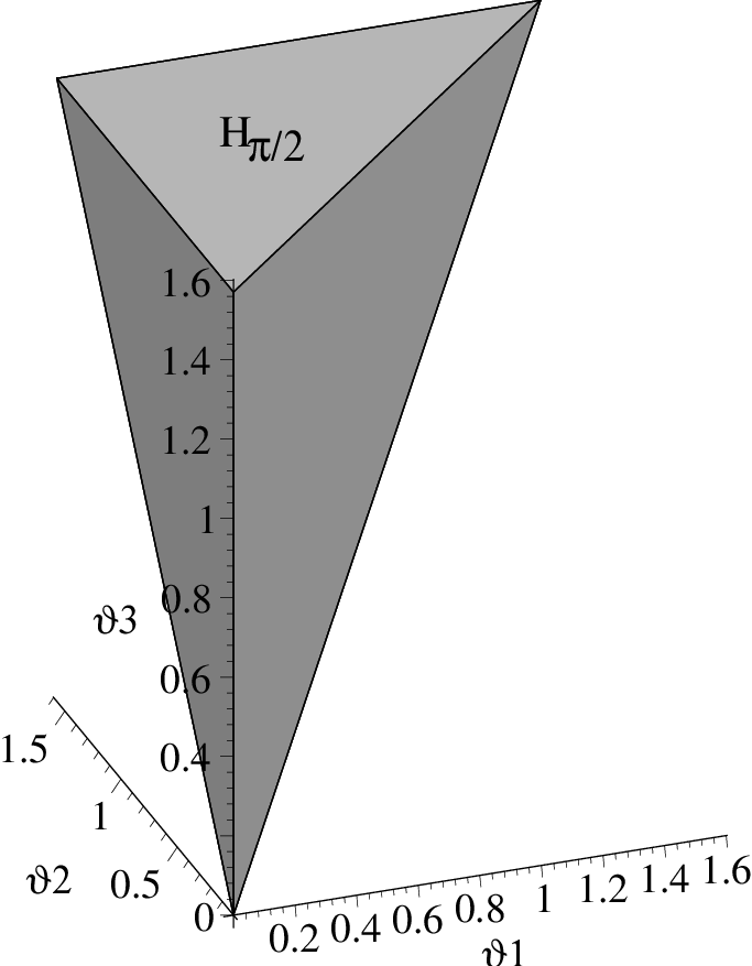
Lagrangian analysis: The non-coherent channel diversity sum and product and the corresponding lower bounds for their coherent channel analogues (by embedding), are functions of type H⁡(ϑ)=∑i=1nth⁡(ϑi)H(\vartheta)=\sum_{i=1}^{n_{t}}h(\vartheta_{i}) or K⁡(ϑ)=∏i=1nth⁡(ϑi)K(\vartheta)=\prod_{i=1}^{n_{t}}h(\vartheta_{i}) with either h=sin2h=\sin^{2} (for d 2\smash[b]{\underset{\rule[5.0pt]{2.2604pt}{0.25pt}}{d}}^{2} (29), p 2\smash[b]{\underset{\rule[5.0pt]{2.2604pt}{0.25pt}}{p}}^{2} (44)) or h=2​(1−cos)h=2(1-\cos) (for d ​dist2\smash[t]{\overset{\rule[-0.5pt]{2.2604pt}{0.25pt}}{d}}\mathrm{dist}^{2} (49), p ​dist2\smash[t]{\overset{\rule[-0.5pt]{2.2604pt}{0.25pt}}{p}}\mathrm{dist}^{2} (50)). Their domain of definition is the closed simplex Θ \smash[t]{\overset{\rule[-0.5pt]{2.2604pt}{0.25pt}}{\Theta}} of principal angles (see figure 1)

Θ :={ϑ=(ϑ1,…,ϑnt)| 0≤ϑ1≤⋯≤ϑnt≤π2}\smash[t]{\overset{\rule[-0.5pt]{2.2604pt}{0.25pt}}{\Theta}}:=\left\{\left.\vartheta=(\vartheta_{1},\dots,\vartheta_{n_{t}})\>\right|\>0\leq\vartheta_{1}\leq\cdots\leq\vartheta_{n_{t}}\leq\frac{\pi}{2}\right\} (63)

(the open simplex being Θ:={ϑ∈ℝnt| 0<ϑ1<⋯<ϑnt<π/2}\Theta:=\{\vartheta\in\mathds{R}^{n_{t}}\,|\,0<\vartheta_{1}<\cdots<\vartheta_{n_{t}}<\pi/2\})

Refer to caption
Fig. 1: Θ¯\bar{\Theta} for nt=3n_{t}=3

but since the principal angles vary like the identity map id\id for 0≤ϑi≤π/20\leq\vartheta_{i}\leq\pi/2 but extend to π−id\pi-\id for π/2<ϑi<π\pi/2<\vartheta_{i}<\pi (considered as a function on the aperture angle), the function hh (i.e. 1−cos1-\cos) fails in general to be differentiable transversal to the closed facet Hπ/2H_{\pi/2} of Θ \smash[t]{\overset{\rule[-0.5pt]{2.2604pt}{0.25pt}}{\Theta}} containing ϑnt=π/2\vartheta_{n_{t}}=\pi/2. Transversal to any other edge hh is smooth, of course. In order to apply the classical Lagrangian formalism of constrained optimization problems in ℝnt\mathds{R}^{n_{t}} to the present situation, we must convince ourselves, that the non-smooth edges and the π/2\pi/2-facet of Θ \smash[t]{\overset{\rule[-0.5pt]{2.2604pt}{0.25pt}}{\Theta}} do not interfere. Our next task therefore consists of an appropriate decomposition of Θ \smash[t]{\overset{\rule[-0.5pt]{2.2604pt}{0.25pt}}{\Theta}} into smooth pieces, which decompose the optimization into a series of smaller tasks of one single type, solvable simultaneously in ℝl\mathds{R}^{l}, l≤ntl\leq n_{t} (formula (67) shows the resulting problem formulation).

We need a little bit more notation. Let Θ <:=Θ ∖Hπ/2\smash[t]{\overset{\rule[-0.5pt]{2.2604pt}{0.25pt}}{\Theta}}_{<}:=\smash[t]{\overset{\rule[-0.5pt]{2.2604pt}{0.25pt}}{\Theta}}\setminus H_{\pi/2}, and ∂Θ<:=Θ <∖Θ\partial\Theta_{<}:=\smash[t]{\overset{\rule[-0.5pt]{2.2604pt}{0.25pt}}{\Theta}}_{<}\setminus\Theta the C0C^{0} boundary manifold of Θ\Theta with the problematic facet removed. For l=0,…,kl=0,\dots,k the faces contained in Θ <\smash[t]{\overset{\rule[-0.5pt]{2.2604pt}{0.25pt}}{\Theta}}_{<} of dimension ll are given by

∂(l)Θ<:={0=ϑ1=⋯=ϑp1<ϑp1+1=⋯=ϑp2⋮<ϑpl+1=⋯=ϑnt|p1<⋯<plpi=i−1​…​nt−(l−i+1)}\begin{split}&\partial^{(l)}\Theta_{<}:=\\ &\left\{\left.\begin{aligned} 0&=\vartheta_{1}=\dots=\vartheta_{p_{1}}\\ &<\vartheta_{p_{1}+1}=\dots=\vartheta_{p_{2}}\\ &\quad\vdots\\ &<\vartheta_{p_{l}+1}=\dots=\vartheta_{n_{t}}\end{aligned}\,\right|\,\begin{gathered}p_{1}<\dots<p_{l}\\ p_{i}=i-1\dots n_{t}-(l-i+1)\end{gathered}\right\}\end{split}

thus ∂(l)Θ<\partial^{(l)}\Theta_{<} consists exactly of those faces in Θ <\smash[t]{\overset{\rule[-0.5pt]{2.2604pt}{0.25pt}}{\Theta}}_{<}, which are given by p1p_{1} (possibly =0=0) zero angles followed by ll ’blocks’ each of equal nonzero angles, in increasing order, in particular ∂(0)Θ<={0}\partial^{(0)}\Theta_{<}=\{0\}, ∂(nt)Θ<=Θ\partial^{(n_{t})}\Theta_{<}=\Theta. Each face ∂(l)Θ<\partial^{(l)}\Theta_{<} is a smooth submanifold of ∂Θ<\partial\Theta_{<}, with ∂(∂(l)Θ<)=∂(l−1)Θ<\partial(\partial^{(l)}\Theta_{<})=\partial^{(l-1)}\Theta_{<} and Θ <=∪˙l=1nt​∂(l)Θ<\smash[t]{\overset{\rule[-0.5pt]{2.2604pt}{0.25pt}}{\Theta}}_{<}=\dot{\cup}_{l=1}^{n_{t}}\partial^{(l)}\Theta_{<}. The tangent spaces are

T⁡(∂(l)Θ<)={∑i=1lλi(epi+1+⋯+epi+1)|λi∈ℝp1<⋯<pl<pl+1=ntpi=i−1​…​nt−(l−i+1)}\begin{split}&T\left(\partial^{(l)}\Theta_{<}\right)=\\ &\left\{\!\sum_{i=1}^{l}\lambda_{i}(e_{p_{i}+1}+\dots+e_{p_{i+1}})\left|\begin{gathered}\lambda_{i}\in\mathds{R}\\ p_{1}<\dots<p_{l}<p_{l+1}=n_{t}\\ p_{i}=i-1\dots n_{t}-(l-i+1)\end{gathered}\right.\!\!\right\}\end{split}

Then we have

Lemma IV.1

Given H⁡(ϑ)=∑i=1nth⁡(ϑi)H(\vartheta)=\sum_{i=1}^{n_{t}}h(\vartheta_{i}), K⁡(ϑ)=∏i=1nth⁡(ϑi)K(\vartheta)=\prod_{i=1}^{n_{t}}h(\vartheta_{i}) on Θ <\smash[t]{\overset{\rule[-0.5pt]{2.2604pt}{0.25pt}}{\Theta}}_{<} with h∈C∞([0,π/2[)h\in C^{\infty}([0,\pi/2[) (this means, that hh is differentiable from the right in 00) and h′​(0)=0h^{\prime}(0)=0. Then for l=0,…,ntl=0,\dots,n_{t}

gradH|∂(l)Θ<∈T(∂(l)Θ<)\displaystyle\grad H_{|\partial^{(l)}\Theta_{<}}\in T\left(\partial^{(l)}\Theta_{<}\right) (64)
gradK|∂(l)Θ<∈T(∂(l)Θ<)\displaystyle\grad K_{|\partial^{(l)}\Theta_{<}}\in T\left(\partial^{(l)}\Theta_{<}\right) (65)

thus restricting the gradients remains intrinsic.

Proof.

We have grad⁡H⁡(ϑ)=(h′​(ϑ1),…,h′​(ϑnt))\grad H(\vartheta)=(h^{\prime}(\vartheta_{1}),\dots,h^{\prime}(\vartheta_{n_{t}})). Since h′​(0)=0h^{\prime}(0)=0 the symmetry of HH ensures
gradH|∂(l)Θ<(ϑ)=∑i=1lh′(ϑpi+1)(epi+1+⋯+epi+1)∈T(∂(l)Θ<)\grad H_{|\partial^{(l)}\Theta_{<}}(\vartheta)=\sum_{i=1}^{l}h^{\prime}(\vartheta_{p_{i}+1})(e_{p_{i}+1}+\dots+e_{p_{i+1}})\in T\left(\partial^{(l)}\Theta_{<}\right), with λi=h′​(ϑpi+1)\lambda_{i}=h^{\prime}(\vartheta_{p_{i}+1}). Similarly, grad⁡K⁡(ϑ)=(h′​(ϑi)​∏j≠ih⁡(ϑj))i\grad K(\vartheta)=(h^{\prime}(\vartheta_{i})\prod_{j\neq i}h(\vartheta_{j}))_{i}, thus gradK|∂(l)Θ<(ϑ)=0\grad K_{|\partial^{(l)}\Theta_{<}}(\vartheta)=0 (for p1>0p_{1}>0) or gradK|∂(l)Θ<(ϑ)=∑i=1lλi(epi+1+⋯+epi+1)∈T(∂(l)Θ<)\grad K_{|\partial^{(l)}\Theta_{<}}(\vartheta)=\sum_{i=1}^{l}\lambda_{i}(e_{p_{i}+1}+\dots+e_{p_{i+1}})\in T\left(\partial^{(l)}\Theta_{<}\right) with
λi=h′​(ϑpi+1)​h​(ϑpi+1)pi+1−pi−1​∏j≠ih​(ϑpj+1)pj+1−pj\lambda_{i}=h^{\prime}(\vartheta_{p_{i}+1})h(\vartheta_{p_{i}+1})^{p_{i+1}-p_{i}-1}\prod_{j\neq i}h(\vartheta_{p_{j}+1})^{p_{j+1}-p_{j}}. ∎

The lemma ensures, that the Lagrangian functional F=f−λ⁡(g−δ)F=f-\lambda(g-\delta) on a neighborhood of Θ \smash[t]{\overset{\rule[-0.5pt]{2.2604pt}{0.25pt}}{\Theta}} for critical points of ff obeying the constraint g=δg=\delta (f,gf,g either HH or KK, δ∈ℝ\delta\in\mathds{R}) applies to the boundary ∂Θ<\partial\Theta_{<}. Since ff and gg are not necessarily differentiable transversal to Hπ/2H_{\pi/2}, extremal points in Θ \smash[t]{\overset{\rule[-0.5pt]{2.2604pt}{0.25pt}}{\Theta}} lie in the set {g=δ}∩Hπ/2∪Θ <∩{DF=0}\{g=\delta\}\cap H_{\pi/2}\>\cup\>\smash[t]{\overset{\rule[-0.5pt]{2.2604pt}{0.25pt}}{\Theta}}_{<}\cap\{DF=0\} (recall, that ∩\cap has higher precedence than ∪\cup and DD denotes differentiation). For a more unified treatment we define Θ (l):={0≤ϑ1≤⋯≤ϑl≤π/2}\smash[t]{\overset{\rule[-0.5pt]{2.2604pt}{0.25pt}}{\Theta}}^{(l)}:=\{0\leq\vartheta_{1}\leq\cdots\leq\vartheta_{l}\leq\pi/2\} (in particular Θ (0)=∅\smash[t]{\overset{\rule[-0.5pt]{2.2604pt}{0.25pt}}{\Theta}}^{(0)}=\emptyset and Θ (nt)=Θ \smash[t]{\overset{\rule[-0.5pt]{2.2604pt}{0.25pt}}{\Theta}}^{(n_{t})}=\smash[t]{\overset{\rule[-0.5pt]{2.2604pt}{0.25pt}}{\Theta}}) and recall, that on the one hand ff, gg are differentiable tangential to Hπ/2H_{\pi/2} and on the other hand Θ l−1∪{ϑl=⋯=ϑnt=π/2}\smash[t]{\overset{\rule[-0.5pt]{2.2604pt}{0.25pt}}{\Theta}}^{l-1}\cup\{\vartheta_{l}=\dots=\vartheta_{n_{t}}=\pi/2\}, l=1,…,nt−1l=1,\dots,n_{t}-1 exhausts Hπ/2H_{\pi/2}. This leads to the following recursion scheme: For l=0,…,ntl=0,\dots,n_{t} set

H(l)​(ϑ1,…,ϑl)=∑i=1lh⁡(ϑi)+h⁡(π2)​(nt−l)\displaystyle H^{(l)}(\vartheta_{1},\dots,\vartheta_{l})=\sum_{i=1}^{l}h(\vartheta_{i})+h(\tfrac{\pi}{2})(n_{t}-l) (66)
K(l)​(ϑ1,…,ϑl)=∏i=1lh⁡(ϑi)⋅h​(π2)(nt−l)\displaystyle K^{(l)}(\vartheta_{1},\dots,\vartheta_{l})=\prod_{i=1}^{l}h(\vartheta_{i})\cdot h(\tfrac{\pi}{2})^{(n_{t}-l)}

and f(l),g(l)f^{(l)},g^{(l)} given by either H(l)H^{(l)} or K(l)K^{(l)}. Then the extremal points in Θ \smash[t]{\overset{\rule[-0.5pt]{2.2604pt}{0.25pt}}{\Theta}} lie in the set

⋃l=0nt({DF(l)=0}∩Θ <(l)∪{ϑl+1=⋯=ϑnt=π2})\bigcup_{l=0}^{n_{t}}\left(\{DF^{(l)}=0\}\cap\smash[t]{\overset{\rule[-0.5pt]{2.2604pt}{0.25pt}}{\Theta}}^{(l)}_{<}\cup\{\vartheta_{l+1}=\dots=\vartheta_{n_{t}}=\frac{\pi}{2}\}\right) (67)

whereas F(l):=f(l)−λ⁡(g(l)−δ)F^{(l)}:=f^{(l)}-\lambda(g^{(l)}-\delta). Furthermore, for hh monotonically increasing on [0,π/2][0,\pi/2] and zero at 00, the conditions g(l)=δg^{(l)}=\delta forces δ∈[0,h⁡(π2)​nt]\delta\in[0,h(\tfrac{\pi}{2})n_{t}] (resp. δ∈[0,h​(π2)tn]\delta\in[0,h(\tfrac{\pi}{2})^{n}_{t}]) and in the first case l≥⌈nt−δ/h⁡(π2)⌉=:l l\geq\lceil n_{t}-\delta/h(\tfrac{\pi}{2})\rceil=:\smash[b]{\underset{\rule[5.0pt]{2.2604pt}{0.25pt}}{l}}, thus ll restricts to {l ,…,nt}\{\smash[b]{\underset{\rule[5.0pt]{2.2604pt}{0.25pt}}{l}},\dots,n_{t}\}.

Let us now start the Lagrangian analysis of the diversity (resp. with the analysis of the various diversity sums and products). The non-coherent channel diversity sum/product (d )​(p )(\smash[b]{\underset{\rule[5.0pt]{2.2604pt}{0.25pt}}{d}})(\smash[b]{\underset{\rule[5.0pt]{2.2604pt}{0.25pt}}{p}}) as well as the lower bounds (d ​dist)​(p ​dist)(\smash[t]{\overset{\rule[-0.5pt]{2.2604pt}{0.25pt}}{d}}\mathrm{dist})(\smash[t]{\overset{\rule[-0.5pt]{2.2604pt}{0.25pt}}{p}}\mathrm{dist}) for the coherent channel analogues depend on the U⁡(nt)U(n_{t})-fibers only (moreover they depend only on the principal angles). By left invariance we can always assume Ψ=(𝟏𝟎)\Psi=\left(\begin{smallmatrix}\mathbf{1}\\ \mathbf{0}\end{smallmatrix}\right) and consider the diversity terms as functions (marked with an 0 {}_{\smash[b]{\underset{\rule[5.0pt]{1.61458pt}{0.25pt}}{0}}}) on the single argument Φ\Phi, for which ⟨Φ⟩\left\langle\Phi\right\rangle is separated by principal angles ϑ∈Θ \vartheta\in\smash[t]{\overset{\rule[-0.5pt]{2.2604pt}{0.25pt}}{\Theta}} from ⟨(𝟏𝟎)⟩\left\langle\left(\begin{smallmatrix}\mathbf{1}\\ \mathbf{0}\end{smallmatrix}\right)\right\rangle.
𝒑 𝟎 |𝑺𝒅 𝟐​(𝜹)𝟐\boldsymbol{{\smash[b]{\underset{\rule[5.0pt]{2.33331pt}{0.25pt}}{p}}}_{\smash[b]{\underset{\rule[5.0pt]{1.66666pt}{0.25pt}}{0}}\big|S_{\smash[b]{\underset{\rule[5.0pt]{1.66666pt}{0.25pt}}{d}}^{2}}(\delta)}^{2}}:
In order to find the maximum of p \smash[b]{\underset{\rule[5.0pt]{2.2604pt}{0.25pt}}{p}} in the unit distance sphere we constrain f=p 0 2=∏isin2f={\smash[b]{\underset{\rule[5.0pt]{2.2604pt}{0.25pt}}{p}}}_{\smash[b]{\underset{\rule[5.0pt]{1.61458pt}{0.25pt}}{0}}}^{2}=\prod_{i}\sin^{2} on Sd 2​(δ)S_{\smash[b]{\underset{\rule[5.0pt]{1.61458pt}{0.25pt}}{d}}^{2}}(\delta), by setting g=d 0 2=∑isin2g={\smash[b]{\underset{\rule[5.0pt]{2.2604pt}{0.25pt}}{d}}}_{\smash[b]{\underset{\rule[5.0pt]{1.61458pt}{0.25pt}}{0}}}^{2}=\sum_{i}\sin^{2}. Thus we get the Lagrangian functional F⁡(ϑ)=∏isin2⁡ϑi−λ⁡(∑isin2⁡ϑi−δ)F(\vartheta)=\prod_{i}\sin^{2}\vartheta_{i}-\lambda(\sum_{i}\sin^{2}\vartheta_{i}-\delta), 0<δ≤nt0<\delta\leq n_{t}. Here we have l =⌈nt−δ⌉\smash[b]{\underset{\rule[5.0pt]{2.2604pt}{0.25pt}}{l}}=\lceil n_{t}-\delta\rceil and from (67) we get for each l∈{l ,…,nt}l\in\{\smash[b]{\underset{\rule[5.0pt]{2.2604pt}{0.25pt}}{l}},\dots,n_{t}\}

{DF(l)=0}∩Θ (l)<={g(l)=δ}∩{0=ϑ1=⋯=ϑp1<ϑp1+1≤⋯≤ϑl<π2|λ=∏i≠jlsin2ϑi,∀p1<j≤l}\begin{split}&\{DF^{(l)}=0\}\cap\smash[t]{\overset{\rule[-0.5pt]{2.2604pt}{0.25pt}}{\Theta}}^{(l)}_{<}=\left\{g^{(l)}=\delta\right\}\,\cap\\ &\left\{\left.\begin{aligned} 0&=\vartheta_{1}=\dots=\vartheta_{p_{1}}\\ &<\vartheta_{p_{1}+1}\leq\dots\leq\vartheta_{l}<\frac{\pi}{2}\end{aligned}\,\right|\lambda=\prod_{i\neq j}^{l}\sin^{2}\vartheta_{i},\,\forall_{p_{1}<j\leq l}\right\}\end{split}

From this we get extremal points with f≠0f\neq 0 only for p1=0p_{1}=0, ϑ1=⋯=ϑl=θ(l)\vartheta_{1}=\dots=\vartheta_{l}=\theta^{(l)} with l​sin2⁡θ(l)=δ−(nt−l)l\sin^{2}\theta^{(l)}=\delta-(n_{t}-l) and f(l)=(sin2⁡θ(l))l=(1−nt−δl)lf^{(l)}=(\sin^{2}\theta^{(l)})^{l}=(1-\tfrac{n_{t}-\delta}{l})^{l}, monotonically increasing with ll, therefore

max⁡p 0 |Sd 2​(δ)2=f(nt)=(δnt)nt\max{\smash[b]{\underset{\rule[5.0pt]{2.2604pt}{0.25pt}}{p}}}_{\smash[b]{\underset{\rule[5.0pt]{1.61458pt}{0.25pt}}{0}}\big|S_{\smash[b]{\underset{\rule[5.0pt]{1.61458pt}{0.25pt}}{d}}^{2}}(\delta)}^{2}=f^{(n_{t})}=\left(\frac{\delta}{n_{t}}\right)^{n_{t}} (68)

attained in ϑ1=…​ϑnt=θ\vartheta_{1}=\dots\vartheta_{n_{t}}=\theta, sin2⁡θ=δ/nt\sin^{2}\theta=\delta/n_{t}.

Conclusion IV.2

Locally the code points of 𝒞G{\cal C}^{G} for the non-coherent channel have to be distributed with as many of their pairwise principal angles to be nonzero and equal in modulus as possible.

In principle, the same holds for the coherent channel, if we consider p \smash[t]{\overset{\rule[-0.5pt]{2.2604pt}{0.25pt}}{p}} and d \smash[t]{\overset{\rule[-0.5pt]{2.2604pt}{0.25pt}}{d}} as functions of σ {\smash[t]{\overset{\rule[-0.5pt]{2.2604pt}{0.25pt}}{\sigma}}}: The maximum diversity product is attained for σ 1=⋯=σ nt=𝔰{\smash[t]{\overset{\rule[-0.5pt]{2.2604pt}{0.25pt}}{\sigma}}}_{1}=\dots={\smash[t]{\overset{\rule[-0.5pt]{2.2604pt}{0.25pt}}{\sigma}}}_{n_{t}}=\mathfrak{s}, 𝔰2=δ/nt\mathfrak{s}^{2}=\delta/n_{t}, p 2=𝔰2​nt=(δ/nt)nt\smash[t]{\overset{\rule[-0.5pt]{2.2604pt}{0.25pt}}{p}}^{2}=\mathfrak{s}^{2n_{t}}=(\delta/n_{t})^{n_{t}}, but it seems difficult to characterize all Φ∈Sd 2​(δ)\Phi\in S_{\smash[t]{\overset{\rule[-0.5pt]{1.61458pt}{0.25pt}}{d}}^{2}}(\delta) subject to σ 1=…​σ nt=𝔰{\smash[t]{\overset{\rule[-0.5pt]{2.2604pt}{0.25pt}}{\sigma}}}_{1}=\dots{\smash[t]{\overset{\rule[-0.5pt]{2.2604pt}{0.25pt}}{\sigma}}}_{n_{t}}=\mathfrak{s}. Let us embed 𝒞G{\cal C}^{G} into Vnt,TℂV^{\mathds{C}}_{n_{t},T} instead and investigate the question, which conditions have to be imposed on 𝒞G{\cal C}^{G} in order to achieve some diversity gain in terms of d ​dist\smash[t]{\overset{\rule[-0.5pt]{2.2604pt}{0.25pt}}{d}}\mathrm{dist} and p ​dist\smash[t]{\overset{\rule[-0.5pt]{2.2604pt}{0.25pt}}{p}}\mathrm{dist}.
𝒅 ​𝐝𝐢𝐬𝐭𝟎 |𝑺𝒅 𝟐​(𝜹)𝟐\boldsymbol{\smash[t]{\overset{\rule[-0.5pt]{2.33331pt}{0.25pt}}{d}}\mathrm{dist}^{2}_{\smash[b]{\underset{\rule[5.0pt]{1.66666pt}{0.25pt}}{0}}\big|S_{\smash[b]{\underset{\rule[5.0pt]{1.66666pt}{0.25pt}}{d}}^{2}}(\delta)}}:
For the metric fiber distance d ​dist\smash[t]{\overset{\rule[-0.5pt]{2.2604pt}{0.25pt}}{d}}\mathrm{dist} constrained on Sd 2​(δ)S_{\smash[b]{\underset{\rule[5.0pt]{1.61458pt}{0.25pt}}{d}}^{2}}(\delta) the Lagrangian functional reads F⁡(ϑ)=d ​dist0 2​(ϑ)−λ⁡(d 0 2​(ϑ)−δ)=2​k−2​∑icos⁡ϑi−λ⁡(∑isin2⁡ϑi−δ)F(\vartheta)=\smash[t]{\overset{\rule[-0.5pt]{2.2604pt}{0.25pt}}{d}}\mathrm{dist}^{2}_{\smash[b]{\underset{\rule[5.0pt]{1.61458pt}{0.25pt}}{0}}}(\vartheta)-\lambda({\smash[b]{\underset{\rule[5.0pt]{2.2604pt}{0.25pt}}{d}}}_{\smash[b]{\underset{\rule[5.0pt]{1.61458pt}{0.25pt}}{0}}}^{2}(\vartheta)-\delta)=2k-2\sum_{i}\cos\vartheta_{i}-\lambda(\sum_{i}\sin^{2}\vartheta_{i}-\delta). Again we have 0<δ≤nt0<\delta\leq n_{t}, l =⌈nt−δ⌉\smash[b]{\underset{\rule[5.0pt]{2.2604pt}{0.25pt}}{l}}=\lceil n_{t}-\delta\rceil and from (67) we now get for each l∈{l ,…,nt}l\in\{\smash[b]{\underset{\rule[5.0pt]{2.2604pt}{0.25pt}}{l}},\dots,n_{t}\}

{DF(l)=0}∩Θ (l)<={g(l)=δ}∩{0=ϑ1=⋯=ϑp1<ϑp1+1≤⋯≤ϑl<π2|λ=1cos⁡ϑj,∀p1<j≤l}\begin{split}&\{DF^{(l)}=0\}\cap\smash[t]{\overset{\rule[-0.5pt]{2.2604pt}{0.25pt}}{\Theta}}^{(l)}_{<}=\left\{g^{(l)}=\delta\right\}\,\cap\\ &\left\{\left.\begin{aligned} 0&=\vartheta_{1}=\dots=\vartheta_{p_{1}}\\ &<\vartheta_{p_{1}+1}\leq\dots\leq\vartheta_{l}<\frac{\pi}{2}\end{aligned}\,\right|\lambda=\frac{1}{\cos\vartheta_{j}}\>,\>\>\forall_{p_{1}<j\leq l}\right\}\end{split}

Extremal points are contained in 0=ϑ1=⋯=ϑp10=\vartheta_{1}=\dots=\vartheta_{p_{1}}, ϑp1+1=⋯=ϑl=θ(l)\vartheta_{p_{1}+1}=\dots=\vartheta_{l}=\theta^{(l)} subject to (l−p1)​sin2⁡θ(l)=δ−(nt−l)(l-p_{1})\sin^{2}\theta^{(l)}=\delta-(n_{t}-l) for l=l =⌈nt−δ⌉,…,ntl=\smash[b]{\underset{\rule[5.0pt]{2.2604pt}{0.25pt}}{l}}=\lceil n_{t}-\delta\rceil,\dots,n_{t} and p1=0,…,p 1=⌊nt−δ⌋p_{1}=0,\dots,\smash[t]{\overset{\rule[-0.5pt]{2.2604pt}{0.25pt}}{p}}_{1}=\lfloor n_{t}-\delta\rfloor, with fp1(l)=2​(l−p1)​(1−cos⁡θ(l))+2​(nt−l)=2​(l−p1)​(1−1−q)+2​(nt−l)f^{(l)}_{p_{1}}=2(l-p_{1})(1-\cos\theta^{(l)})+2(n_{t}-l)=2(l-p_{1})(1-\sqrt{1-q})+2(n_{t}-l), q:=δ−nt+ll−p1=sin2⁡θ(l)q:=\tfrac{\delta-n_{t}+l}{l-p_{1}}=\sin^{2}\theta^{(l)}. For fixed ll the function p1⟼fp1(l)p_{1}\longmapsto f^{(l)}_{p_{1}} is monotonically increasing (by analyzing the derivative, where defined) and we find f (l):=minp1⁡fp1(l)=f0(l)\smash[b]{\underset{\rule[5.0pt]{2.2604pt}{0.25pt}}{f}}^{(l)}:=\min_{p_{1}}f^{(l)}_{p_{1}}=f^{(l)}_{0} and f (l):=maxp1⁡fp1(l)=fp1 (l)\smash[t]{\overset{\rule[-0.5pt]{2.2604pt}{0.25pt}}{f}}^{(l)}:=\max_{p_{1}}f^{(l)}_{p_{1}}=f^{(l)}_{\smash[t]{\overset{\rule[-0.5pt]{1.61458pt}{0.25pt}}{p_{1}}}}. As functions of ll both terms turn out to be monotonically decreasing (by analyzing the derivatives with respect to ll) and we find

min⁡d ​dist0 |Sd 2​(δ)2=f (nt)=2​nt​(1−1−δ/nt)\displaystyle\min\smash[t]{\overset{\rule[-0.5pt]{2.2604pt}{0.25pt}}{d}}\mathrm{dist}^{2}_{\smash[b]{\underset{\rule[5.0pt]{1.61458pt}{0.25pt}}{0}}\big|S_{\smash[b]{\underset{\rule[5.0pt]{1.61458pt}{0.25pt}}{d}}^{2}}(\delta)}=\smash[b]{\underset{\rule[5.0pt]{2.2604pt}{0.25pt}}{f}}^{(n_{t})}=2n_{t}\left(1-\sqrt{1-\delta/n_{t}}\right) (69a)
attained in ϑ1=…​ϑnt=θ\vartheta_{1}=\dots\vartheta_{n_{t}}=\theta, sin2⁡θ=δ/nt\sin^{2}\theta=\delta/n_{t}, and
max⁡d ​dist0 |Sd 2​(δ)2=f (l )=2​(1−1−(δ−⌊δ⌋))+2​⌊δ⌋\displaystyle\max\smash[t]{\overset{\rule[-0.5pt]{2.2604pt}{0.25pt}}{d}}\mathrm{dist}^{2}_{\smash[b]{\underset{\rule[5.0pt]{1.61458pt}{0.25pt}}{0}}\big|S_{\smash[b]{\underset{\rule[5.0pt]{1.61458pt}{0.25pt}}{d}}^{2}}(\delta)}=\smash[t]{\overset{\rule[-0.5pt]{2.2604pt}{0.25pt}}{f}}^{(\smash[b]{\underset{\rule[5.0pt]{1.61458pt}{0.25pt}}{l}})}=2\left(1-\sqrt{1-(\delta-\lfloor\delta\rfloor)}\right)+2\lfloor\delta\rfloor (69b)
attained for ϑ1=…​ϑ⌊nt−δ⌋=0\vartheta_{1}=\dots\vartheta_{\lfloor n_{t}-\delta\rfloor}=0, sin2⁡ϑ⌈nt−δ⌉=δ−⌊δ⌋\sin^{2}\vartheta_{\lceil n_{t}-\delta\rceil}=\delta-\lfloor\delta\rfloor, ϑ⌈nt−δ⌉+1=…​ϑnt=π/2\vartheta_{\lceil n_{t}-\delta\rceil+1}=\dots\vartheta_{n_{t}}=\pi/2.

𝒑 ​𝐝𝐢𝐬𝐭𝟎 |𝑺𝒅 𝟐​(𝜹)𝟐\boldsymbol{\smash[t]{\overset{\rule[-0.5pt]{2.33331pt}{0.25pt}}{p}}\mathrm{dist}^{2}_{\smash[b]{\underset{\rule[5.0pt]{1.66666pt}{0.25pt}}{0}}\big|S_{\smash[b]{\underset{\rule[5.0pt]{1.66666pt}{0.25pt}}{d}}^{2}}(\delta)}}:
Examining p ​dist\smash[t]{\overset{\rule[-0.5pt]{2.2604pt}{0.25pt}}{p}}\mathrm{dist} instead of d ​dist\smash[t]{\overset{\rule[-0.5pt]{2.2604pt}{0.25pt}}{d}}\mathrm{dist} we have the Lagrangian F⁡(ϑ)=2k​∏i(1−cos⁡ϑi)−λ⁡(∑isin2⁡ϑi−δ)F(\vartheta)=2^{k}\prod_{i}(1-\cos\vartheta_{i})-\lambda(\sum_{i}\sin^{2}\vartheta_{i}-\delta) and

{DF(l)=0}∩Θ (l)<={g(l)=δ}∩{0=ϑ1=⋯=ϑp1<ϑp1+1≤⋯≤ϑl<π2|λ=2nt−1cos⁡ϑj​∏i≠jl(1−cos⁡ϑi)∀p1<j≤l}\begin{split}&\{DF^{(l)}=0\}\cap\smash[t]{\overset{\rule[-0.5pt]{2.2604pt}{0.25pt}}{\Theta}}^{(l)}_{<}=\left\{g^{(l)}=\delta\right\}\,\cap\\ &\left\{\left.\begin{aligned} 0&=\vartheta_{1}=\dots=\vartheta_{p_{1}}\\ &<\vartheta_{p_{1}+1}\leq\dots\leq\vartheta_{l}<\frac{\pi}{2}\end{aligned}\right|\begin{aligned} \lambda=\frac{2^{n_{t}-1}}{\cos\vartheta_{j}}\prod_{i\neq j}^{l}(1-\cos\vartheta_{i})&\\ \forall_{p_{1}<j\leq l}&\end{aligned}\right\}\end{split}

From this we get extremal points with f≠0f\neq 0 only for p1=0p_{1}=0, ϑ1=⋯=ϑl=θ(l)\vartheta_{1}=\dots=\vartheta_{l}=\theta^{(l)} with l​sin2⁡θ(l)=δ−(nt−l)l\sin^{2}\theta^{(l)}=\delta-(n_{t}-l) and f(l)=2nt​(1−cos⁡θ(l))l=2nt​(1−nt−δl)lf^{(l)}=2^{n_{t}}(1-\cos\theta^{(l)})^{l}=2^{n_{t}}(1-\sqrt{\tfrac{n_{t}-\delta}{l}})^{l}, monotonically increasing with ll and therfore

max⁡p ​dist0 |Sd 2​(δ)2=f(nt)=2nt​(1−1−δ/nt)nt\max\smash[t]{\overset{\rule[-0.5pt]{2.2604pt}{0.25pt}}{p}}\mathrm{dist}^{2}_{\smash[b]{\underset{\rule[5.0pt]{1.61458pt}{0.25pt}}{0}}\big|S_{\smash[b]{\underset{\rule[5.0pt]{1.61458pt}{0.25pt}}{d}}^{2}}(\delta)}=f^{(n_{t})}=2^{n_{t}}\left(1-\sqrt{1-\delta/n_{t}}\right)^{n_{t}} (70)

in ϑ1=…​ϑnt=θ\vartheta_{1}=\dots\vartheta_{n_{t}}=\theta, sin2⁡θ=δ/nt\sin^{2}\theta=\delta/n_{t}.

Remark IV.3

If we had constrained p ​dist\smash[t]{\overset{\rule[-0.5pt]{2.2604pt}{0.25pt}}{p}}\mathrm{dist} on Sd ​dist2​(δ)S_{\smash[t]{\overset{\rule[-0.5pt]{1.61458pt}{0.25pt}}{d}}\mathrm{dist}^{2}}(\delta), 0<δ≤2​nt0<\delta\leq 2n_{t} we would have gotten

max⁡p ​dist0 |Sd ​dist2​(δ)2=(δnt)nt\max\smash[t]{\overset{\rule[-0.5pt]{2.2604pt}{0.25pt}}{p}}\mathrm{dist}^{2}_{\smash[b]{\underset{\rule[5.0pt]{1.61458pt}{0.25pt}}{0}}\big|S_{\smash[t]{\overset{\rule[-0.5pt]{1.61458pt}{0.25pt}}{d}}\mathrm{dist}^{2}}(\delta)}=\left(\frac{\delta}{n_{t}}\right)^{n_{t}} (71)

attained in ϑ1=…​ϑnt=θ\vartheta_{1}=\dots\vartheta_{n_{t}}=\theta, 2​(1−cos⁡θ)=δ/nt2(1-\cos\theta)=\delta/n_{t}, by analogy to the case of p \smash[b]{\underset{\rule[5.0pt]{2.2604pt}{0.25pt}}{p}} constrained on d \smash[b]{\underset{\rule[5.0pt]{2.2604pt}{0.25pt}}{d}}. The apparent discrepancy of (70) to (71) is caused by (69b), since at ϑ1=⋯=ϑnt=θ\vartheta_{1}=\dots=\vartheta_{n_{t}}=\theta d ​dist0 2\smash[t]{\overset{\rule[-0.5pt]{2.2604pt}{0.25pt}}{d}}\mathrm{dist}^{2}_{\smash[b]{\underset{\rule[5.0pt]{1.61458pt}{0.25pt}}{0}}} attains its minimum δ~=2​nt​(1−1−δ/nt)\tilde{\delta}=2n_{t}(1-\sqrt{1-\delta/n_{t}}) on Sd 2​(δ)S_{\smash[b]{\underset{\rule[5.0pt]{1.61458pt}{0.25pt}}{d}}^{2}}(\delta) which yields (with (71)) p ​dist0 |d ​dist0 2=δ~2=(δ~/nt)nt=2nt​(1−1−δ/nt)nt\smash[t]{\overset{\rule[-0.5pt]{2.2604pt}{0.25pt}}{p}}\mathrm{dist}^{2}_{\smash[b]{\underset{\rule[5.0pt]{1.61458pt}{0.25pt}}{0}}|\smash[t]{\overset{\rule[-0.5pt]{1.61458pt}{0.25pt}}{d}}\mathrm{dist}^{2}_{\smash[b]{\underset{\rule[5.0pt]{1.61458pt}{0.25pt}}{0}}}=\tilde{\delta}}=(\tilde{\delta}/n_{t})^{n_{t}}=2^{n_{t}}(1-\sqrt{1-\delta/n_{t}})^{n_{t}}, which coincides with (70).

Conclusion IV.4

What remains is the general rule, that for ϱ =ρ​T4​nt≫1\smash[t]{\overset{\rule[-0.5pt]{2.2604pt}{0.25pt}}{\varrho}}=\tfrac{\rho T}{4n_{t}}\gg 1 (compare (36)) in favor of p ​dist\smash[t]{\overset{\rule[-0.5pt]{2.2604pt}{0.25pt}}{p}}\mathrm{dist} instead of d ​dist\smash[t]{\overset{\rule[-0.5pt]{2.2604pt}{0.25pt}}{d}}\mathrm{dist} one should distribute the pairwise principal angles in 𝒞G{\cal C}^{G} locally to be all nonzero and equal in modulus (by (70)). This coincides with the preferred strategy (68) for the non-coherent channel code. For ϱ ≤1\smash[t]{\overset{\rule[-0.5pt]{2.2604pt}{0.25pt}}{\varrho}}\leq 1, when the higher order diversity terms become less important, it might be better to distribute the pairwise principal angles globally to maximize d ​dist\smash[t]{\overset{\rule[-0.5pt]{2.2604pt}{0.25pt}}{d}}\mathrm{dist}, thus separating points in 𝒞G{\cal C}^{G} by as many of the principal angles to be zero such that the remaining ones attain large values.

𝒑 ​𝐝𝐢𝐬𝐭𝟎 |𝑺𝒑 𝟐​(𝜹)𝟐\boldsymbol{\smash[t]{\overset{\rule[-0.5pt]{2.33331pt}{0.25pt}}{p}}\mathrm{dist}^{2}_{\smash[b]{\underset{\rule[5.0pt]{1.66666pt}{0.25pt}}{0}}\big|S_{\smash[b]{\underset{\rule[5.0pt]{1.66666pt}{0.25pt}}{p}}^{2}}(\delta)}}:
Finally, to get an product analogue of (69) we analyze p ​dist0 2\smash[t]{\overset{\rule[-0.5pt]{2.2604pt}{0.25pt}}{p}}\mathrm{dist}^{2}_{\smash[b]{\underset{\rule[5.0pt]{1.61458pt}{0.25pt}}{0}}} constrained on Sp 2​(δ)S_{\smash[b]{\underset{\rule[5.0pt]{1.61458pt}{0.25pt}}{p}}^{2}}(\delta), 0<δ≤10<\delta\leq 1, thus the Lagrangian reads F⁡(ϑ)=2k​∏i(1−cos⁡ϑi)−λ⁡(∏isin2⁡ϑi−δ)F(\vartheta)=2^{k}\prod_{i}(1-\cos\vartheta_{i})-\lambda(\prod_{i}\sin^{2}\vartheta_{i}-\delta) and for l∈{0,…,nt}l\in\{0,\dots,n_{t}\} we have

{DF(l)=0}∩Θ (l)<={g(l)=δ}∩{0=ϑ1=⋯=ϑp1<ϑp1+1≤⋯≤ϑl<π2|λ=2nt−1cos⁡ϑj​∏i≠jl1−cos⁡ϑisin2⁡ϑi∀p1<j≤l}\begin{split}&\{DF^{(l)}=0\}\cap\smash[t]{\overset{\rule[-0.5pt]{2.2604pt}{0.25pt}}{\Theta}}^{(l)}_{<}=\left\{g^{(l)}=\delta\right\}\,\cap\\ &\left\{\left.\begin{aligned} 0&=\vartheta_{1}=\dots=\vartheta_{p_{1}}\\ &<\vartheta_{p_{1}+1}\leq\dots\leq\vartheta_{l}<\frac{\pi}{2}\end{aligned}\right|\begin{aligned} \lambda=\frac{2^{n_{t}-1}}{\cos\vartheta_{j}}\prod_{i\neq j}^{l}\frac{1-\cos\vartheta_{i}}{\sin^{2}\vartheta_{i}}&\\ \forall_{p_{1}<j\leq l}&\end{aligned}\right\}\end{split}

δ>0\delta>0 forces p1=0p_{1}=0 and we get ϑ1=⋯=ϑl=θ(l)\vartheta_{1}=\dots=\vartheta_{l}=\theta^{(l)}, sin2​l⁡θ(l)=δ\sin^{2l}\theta^{(l)}=\delta, thus f(l)=2nt​(1−cos⁡θ(l))l=2nt​(1−1−δ1/l)lf^{(l)}=2^{n_{t}}(1-\cos\theta^{(l)})^{l}=2^{n_{t}}(1-\sqrt{1-\delta^{1/l}})^{l} which is monotonically decreasing in ll, so

min⁡p ​dist0 |Sp 2​(δ)2=f(nt)=2nt​(1−1−δ1/nt)nt\displaystyle\min\smash[t]{\overset{\rule[-0.5pt]{2.2604pt}{0.25pt}}{p}}\mathrm{dist}^{2}_{\smash[b]{\underset{\rule[5.0pt]{1.61458pt}{0.25pt}}{0}}\big|S_{\smash[b]{\underset{\rule[5.0pt]{1.61458pt}{0.25pt}}{p}}^{2}}(\delta)}=f^{(n_{t})}=2^{n_{t}}\left(1-\sqrt{1-\delta^{1/n_{t}}}\right)^{n_{t}} (72a)
attained in ϑ1=…​ϑnt=θ\vartheta_{1}=\dots\vartheta_{n_{t}}=\theta, sin2⁡θ=δ1/nt\sin^{2}\theta=\delta^{1/n_{t}}, and
max⁡p ​dist0 |Sp 2​(δ)2=f(1)=2nt​(1−1−δ)\displaystyle\max\smash[t]{\overset{\rule[-0.5pt]{2.2604pt}{0.25pt}}{p}}\mathrm{dist}^{2}_{\smash[b]{\underset{\rule[5.0pt]{1.61458pt}{0.25pt}}{0}}\big|S_{\smash[b]{\underset{\rule[5.0pt]{1.61458pt}{0.25pt}}{p}}^{2}}(\delta)}=f^{(1)}=2^{n_{t}}\left(1-\sqrt{1-\delta}\right) (72b)
attained in sin2⁡ϑ1=δ\sin^{2}\vartheta_{1}=\delta, ϑ2=⋯=ϑnt=π/2\vartheta_{2}=\dots=\vartheta_{n_{t}}=\pi/2

(whereas f(0)f^{(0)} is contained in f(1)f^{(1)} when δ=1\delta=1).

Observing, that the minima in (69) and (72) are monotonically increasing in δ\delta we end up with

Proposition IV.5

In the situation of Proposition III.4 we have

d ​dist2​min\displaystyle\smash[t]{\overset{\rule[-0.5pt]{2.2604pt}{0.25pt}}{d}}\mathrm{dist}^{2\min} ≥min⁡d ​dist0 |Sd 2​(d 2​min)2\displaystyle\geq\min\smash[t]{\overset{\rule[-0.5pt]{2.2604pt}{0.25pt}}{d}}\mathrm{dist}^{2}_{\smash[b]{\underset{\rule[5.0pt]{1.61458pt}{0.25pt}}{0}}\big|S_{\smash[b]{\underset{\rule[5.0pt]{1.61458pt}{0.25pt}}{d}}^{2}}(\smash[b]{\underset{\rule[5.0pt]{1.61458pt}{0.25pt}}{d}}^{2\min})} (73)
=2​nt​(1−1−d 2​min/nt)≥d 2​min\displaystyle=2n_{t}\left(1-\sqrt{1-\smash[b]{\underset{\rule[5.0pt]{2.2604pt}{0.25pt}}{d}}^{2\min}/n_{t}}\right)\geq\smash[b]{\underset{\rule[5.0pt]{2.2604pt}{0.25pt}}{d}}^{2\min}
p ​dist2​min\displaystyle\smash[t]{\overset{\rule[-0.5pt]{2.2604pt}{0.25pt}}{p}}\mathrm{dist}^{2\min} ≥min⁡p ​dist0 |Sp 2​(p 2​min)2\displaystyle\geq\min\smash[t]{\overset{\rule[-0.5pt]{2.2604pt}{0.25pt}}{p}}\mathrm{dist}^{2}_{\smash[b]{\underset{\rule[5.0pt]{1.61458pt}{0.25pt}}{0}}\big|S_{\smash[b]{\underset{\rule[5.0pt]{1.61458pt}{0.25pt}}{p}}^{2}}(\smash[b]{\underset{\rule[5.0pt]{1.61458pt}{0.25pt}}{p}}^{2\min})} (74)
=2nt​(1−1−p 2​min1/nt)nt≥p 2​min\displaystyle=2^{n_{t}}\left(1-\sqrt{1-{\smash[b]{\underset{\rule[5.0pt]{2.2604pt}{0.25pt}}{p}}^{2\min}}^{1/n_{t}}}\right)^{n_{t}}\geq\smash[b]{\underset{\rule[5.0pt]{2.2604pt}{0.25pt}}{p}}^{2\min}

The benefit of this proposition is, that it relates d ​distmin\smash[t]{\overset{\rule[-0.5pt]{2.2604pt}{0.25pt}}{d}}\mathrm{dist}^{\min} (resp. p ​distmin\smash[t]{\overset{\rule[-0.5pt]{2.2604pt}{0.25pt}}{p}}\mathrm{dist}^{\min}) directly to d min\smash[b]{\underset{\rule[5.0pt]{2.2604pt}{0.25pt}}{d}}^{\min} (resp. p min\smash[b]{\underset{\rule[5.0pt]{2.2604pt}{0.25pt}}{p}}^{\min}), regardless if the minimum distances (resp. diversity products) are realized by the same pair of points or not.

Proof.

Its only left up to show the second inequality in each formula, which is elementary (setting x:=d 2​minx:=\smash[b]{\underset{\rule[5.0pt]{2.2604pt}{0.25pt}}{d}}^{2\min} or x:=p 2​minx:=\smash[b]{\underset{\rule[5.0pt]{2.2604pt}{0.25pt}}{p}}^{2\min}, respectively):
(73) ⟺1−x/nt≤1−x/2​nt⟺ 1−x/nt≤(1−x/2​nt)2=1−x/nt+x2/4​nt2\;\Longleftrightarrow\;\sqrt{1-x/n_{t}}\leq 1-x/2n_{t}\;\Longleftrightarrow\;1-x/n_{t}\leq(1-x/2n_{t})^{2}=1-x/n_{t}+x^{2}/4n_{t}^{2}.
(74) ⟺1−x1/nt≤1−x1/k/2⟺ 1−x1/nt≤(1−x1/k/2)2=1−x1/nt+x2/nt/4\;\Longleftrightarrow\;\sqrt{1-x^{1/n_{t}}}\leq 1-x^{1/k}/2\;\Longleftrightarrow\;1-x^{1/n_{t}}\leq(1-x^{1/k}/2)^{2}=1-x^{1/n_{t}}+x^{2/n_{t}}/4 ∎

V Conclusions

This work should be seen as a second step towards a geometry based analysis of general space time block codes, inspired by the results in [16], opening the door to potentially high performing space time block codes, when T≫ntT\gg n_{t}. The various estimates and interrelations explored in this work assemble the following overall picture:

  • •

    Diversity monotony: The performance analysis revealed nice embedding properties (with respect to Gnt,Tℂ⊂Vnt,TℂG^{\mathds{C}}_{n_{t},T}\subset V^{\mathds{C}}_{n_{t},T}) of the diversity quantities (Corollaries III.2, III.3, (57)), leading to a diversity growth (Proposition III.4) in the transition from the non-coherent channel to the coherent channel. This turned out to be due to the various invariance properties satisfied by the diversity, though tied to distinct underlying topologies of the coding spaces induced by the maximum likelihood receiver metrics. Moreover, for the diversity sum and product, more explicit estimates have been derived (Proposition IV.5).

  • •

    Complexity reduction: Embeddings of both Gnt,TℂG^{\mathds{C}}_{n_{t},T} and U⁡(nt)U(n_{t}) into Vnt,TℂV^{\mathds{C}}_{n_{t},T} can be used to construct codes on Vnt,TℂV^{\mathds{C}}_{n_{t},T} from ’smaller’ pieces (Theorem III.5), both of them being already in the focus of current research. The other way round, given an non-coherent channel space time code and a ’small’ coherent channel code, the performance of the resulting (larger dimensional) product code on Vnt,TℂV^{\mathds{C}}_{n_{t},T} is lower bounded by the diversity expressions stated in the theorem. Thus the design complexity has been reduced to the smaller problems on Gnt,TℂG^{\mathds{C}}_{n_{t},T} and U⁡(nt)U(n_{t}). Together with Proposition I.1 this opens the door to potentially high performing space time block codes, when T≫ntT\gg n_{t}. As already indicated in the introduction this may be of some importance in the context of space frequency codes also.

  • •

    Localization: The local nature of the higher order diversity quantities turns space time coding into a constrained packing problem. The diversity sum still represents a major criteria, locally superposed by the diversity product as a rigidity constraint: The optimal code in the high SNR regime is packed as ’diagonal’ as possible, uniformly maximizing the principal angles (Conclusion IV.2 and IV.4).

There are still many open issues. Some immediate will be listed next. The explicit bounds of Proposition IV.5 are very coarse and improvements are necessary. Moreover, it would be desirable to obtain further decompositions in Theorem III.5. Furthermore this work has to be related to the differential coding scheme [9], which benefits from high rates compared to non differential codes. Finally it remains the challenge of effective high dimensional code construction (especially for the non-coherent channel) with low complexity decoding properties.

Acknowledgment

I would like to thank Eduard Jorswieck, Peter Jung, and Aydin Sezgin for reading the manuscript and helpful comments.

References

  • [1] V. Tarokh, N. Seshadri, and A. R. Calderbank, “Space-time codes for high data rate wireless communication: Performance criterion and code construction,” IEEE Trans. Inform. Theory, vol. 44, pp. 744–765, 1998.
  • [2] B. M. Hochwald and T. Marzetta, “Unitary space-time modulation for multiple-antenna communications in Rayleigh flat fading,” IEEE Trans. Inform. Theory, vol. 46, pp. 543–565, 2000.
  • [3] S. M. Alamouti, “A simple transmit diversity technique for wireless communications,” IEEE Journal on Select. Areas in Communications, vol. 16, pp. 1451–1458, 1998.
  • [4] V. Tarokh, H. Jafarkhani, and A. R. Calderbank, “Space-time block codes from orthogonal designs,” IEEE Trans. Inform. Theory, vol. 45, pp. 1456–1467, 1999.
  • [5] B. Hassibi and B. M. Hochwald, “High-rate codes that are linear in space and time,” IEEE Trans. Inform. Theory, vol. 48, no. 7, pp. 1804–1824, 2002.
  • [6] R. H. Gohary and T. N. Davidson, “Design of linear dispersion codes: Asymptotic guidelines and their implementation,” IEEE Trans. Wireless Commun., vol. 4, no. 6, pp. 2892–2906, 2005.
  • [7] J.-C. Belfiore, G. Rekaya, and E. Viterbo, “The golden code: A 2×22\times 2 full-rate space-time code with nonvanishing determinants,” IEEE Trans. Inform. Theory, vol. 51, no. 4, pp. 1432–1436, 2005.
  • [8] V. Tarokh, “Existence and construction of non-coherent unitary space-time codes,” preprint, url: http://www.mit.edu/˜vahid/sample.html.
  • [9] B. M. Hochwald and W. Sweldens, “Differential unitary space-time modulation,” IEEE Trans. Comm., vol. 48, pp. 2041–2052, 2000.
  • [10] A. Shokrollahi, B. Hassibi, B. M. Hochwald, and W. Sweldens, “Representation theory for high-rate multiple-antenna code design,” IEEE Trans. Inform. Theory, vol. 47, pp. 335–2367, 2001.
  • [11] G. Han and J. Rosenthal, “Unitary space time constellation analysis: An upper bound for the diversity,” 2004, preprint arXiv:math.CO/0401045.
  • [12] X.-B. Liang and X.-G. Xia, “Unitary signal constellations for differential space-time modulation with two transmit antennas: Parametric codes, optimal designs, and bounds,” IEEE Trans. Inform. Theory, vol. 48, no. 8, pp. 2291–2322, 2002.
  • [13] H. Wang, G. Wang, and X.-G. Xia, “Some 2×22\times 2 unitary space-time codes from sphere packing theory with optimal diversity product of code size 6,” IEEE Trans. Inform. Theory, vol. 50, no. 12, pp. 3361–3368, 2004.
  • [14] B. M. Hochwald and T. Marzetta, “Capacity of a mobile multiple-antenna communication link in Rayleigh flat fading,” IEEE Trans. Inform. Theory, vol. 45, pp. 139–157, 1999.
  • [15] A. Barg and D. Y. Nogin, “Bounds on packings of spheres in the Grassmann manifold,” IEEE Trans. Inform. Theory, vol. 48, pp. 2450–2454, 2002.
  • [16] O. Henkel, “Sphere packing bounds in the Grassmann and Stiefel manifolds,” IEEE Trans. Inform. Theory, vol. 51, no. 10, pp. 3445–3456, 2005.
  • [17] ——, “Space time codes from permutation codes,” in Proceedings of IEEE GlobeCom 2006, San Francisco, California, 2006.
  • [18] H. Bölcskei, M. Borgmann, and A. J. Paulraj, “Space-Frequency coded MIMO-OFDM with variable multiplexing-diversity tradeoff,” in IEEE International Conference on Communications (ICC’03), vol. 4, 2003, pp. 2837– 2841.
  • [19] H. Bölcskei and M. Borgmann, “Code design for non-coherent MIMO-OFDM systems,” in Proc. 40th Allerton Conf. Commun., Contr., Comput., Monticello, IL, 2002, pp. 237–246.
  • [20] O. Henkel, “Space frequency codes from spherical codes,” in Proceedings of the 2005 IEEE International Symposium on Information Theory (ISIT 05), 2005, pp. 1305–1309. [Online]. Available: http://arxiv.org/abs/cs.IT/0501085
  • [21] I. Kammoun and J.-C. Belfiore, “A new family of Grassmann space-time codes for non-coherent MIMO systems,” IEEE Comm. Letters, vol. 7, no. 11, pp. 528–530, 2003.
  • [22] W. M. Boothby, An Introduction to Differentiable Manifolds and Riemannian Geometry, ser. Pure and Applied Mathematics 120. Academic Press, Inc., Orlando, FL, 1986.
  • [23] L. Conlon, Differentiable Manifolds: A first course. Birkhäuser Boston, 1993.
  • [24] S. Gallot, D. Hulin, and J. Lafontaine, Riemannian Geometry, 2nd ed. Springer, 1993.
  • [25] W. A. Poor, Differential Geometric Structures. McGraw-Hill Inc., 1981.
  • [26] A. Edelman, T. A. Arias, and S. T. Smith, “The geometry of algorithms with orthogonality constraints,” SIAM J. Matrix Anal. Appl., vol. 20, pp. 303–353, 1998.
  • [27] L. Zheng and D. N. C. Tse, “Communication on the Grassmann manifold: a geometric approach to the noncoherent multiple-antenna channel,” IEEE Trans. Inform. Theory, vol. 48, pp. 359–383, 2002.
  • [28] E. Telatar, “Capacity of multi-antenna gaussian channels,” European Transactions on Telecommunications, vol. 10, pp. 585–595, 1999.
  • [29] Å. Björck and G. H. Golub, “Numerical methods for computing angles between linear subspaces,” Mathematics of Computation, vol. 27, no. 123, pp. 579–594, 1973.
  • [30] J. H. Conway, R. H. Hardin, and N. J. A. Sloane, “Packing lines, planes, etc.: Packings in Grassmannian spaces,” Experimental Mathematics, vol. 5, pp. 139–159, 1996. [Online]. Available: http://www.research.att.com/∼\simnjas/grass/index.html
  • [31] R. Bhatia, Matrix Analysis. Springer, 1997.
  • [32] O. Henkel and G. Wunder, “Space frequency codes from sphere packings,” in Proceedings International ITG/IEEE Workshop on Smart Antennas (WSA 2005), Duisburg-Essen, Germany, Apr 2005.