Sensing Capacity for Markov Random Fields

We investigate how spatial Markov structure in the environment affects the number of sensors required to sense that environment to within a desired accuracy. We explore this relationship in the context of discrete sensor network applications such as distributed detection and classification. The number of sensors required to achieve a desired performance level depends the characteristics of the environment (e.g. target sparsity, likely target configurations, target contiguity), the constituent sensors (e.g. noise, range, sensing function), and the resource constraints at sensor nodes (e.g. power, computation, communications). Resource constraints such as communications and power are important to consider in the design of sensor networks due to the limitations they impose on, among other things, network lifetime and sampling rate. See, for example, [1, 2, 3] for a discussion on the effects of resource constraints on sensor networks. However, even if these resource constraints were eliminated, many basic questions about the theoretical design limitations of sensor networks are not yet adequately addressed. The sensing capabilities of the sensors, the spatial characteristics of the environment being sensed, and the required accuracy of the sensing task impose sharp limitations on the number of sensors required to achieve a desired performance level. We elucidate this purely sensing-based limitation, by demonstrating a lower bound on the minimum number of sensors required to achieve a desired sensing performance, given the sensing capabilities of the sensors and a spatial Markov model of the environment. External constraints, such as power, communication, bandwidth, and computation are not considered in this paper.

We model the presence/absence of targets in a two-dimensional grid as a Markov random field [4], and the sensor network as a ‘channel encoder’ (Figure 1). This ‘encoder’ maps the grid of targets into a vector of sensor outputs, which corresponds to a “codeword.” These sensor outputs are then corrupted by noise. The decoder observes this noisy codeword and provides an estimate of the spatial target configuration. Viewing the sensor network as a channel encoder allows us to use ideas from Shannon coding theory. However the messages do not necessarily occur with equal probability, unlike messages in classical channel codes. In addition, as we will show, the “codebook” obtained has codewords which are neither independent nor identical. These differences require a novel analysis and a novel concept of ‘sensing capacity’ $C(D)$. The distortion $D$ is the maximum tolerable fraction of spatial positions which may be erroneously sensed. For a given $D$, $C(D)$ represents the maximum ratio of the total number of target positions under observation to the number of sensors, such that below this ratio, there exist sensor networks whose average probability of error goes to zero as the number of possible target positions and sensors goes to infinity.

In previous work [5], we introduced the concept of a sensing capacity. We extended this work in [6] to account for arbitrary sensing functions and localized sensing of a one-dimensional target vector, with i.i.d. targets. In this paper we explore the effect of Markov structure in a two-dimensional environment on the sensing capacity, as occurs in several practical applications (e.g. robotic demining and prospecting, distributed surveillance). We model the environment as a Markov random field, and show an extension of the theory of types to include Markov random fields. Section II introduces and motivates our sensor network model. Section III states a lower bound on sensing capacity for the model. Illustrative calculations of the sensing capacity appear in Section IV.

We denote random variables and functions by upper-case letters, and instantiations or constants by lower-case letters. Bold-font denotes vectors. $\log(\cdot)$ has base-2. Sets are denoted using calligraphic script. $D(P||Q)$ denotes the Kullback-Leibler distance and $H(P)$ denotes entropy.

We consider the problem of sensing discrete two dimensional environments with spatial structure. Examples include camera networks that localize people in a room, seismic sensor networks that localize moving objects, minefield mapping, and soil mapping. There exists a large body of work in distributed detection [7], but we are not aware of the existence of any ‘sensing capacity’ results. [8] introduced the idea of viewing sensor networks as encoders, and used algebraic coding theory to design highly structured sensor networks, but no notion of capacity was discussed.

The model we present attempts to abstractly characterize the discrete sensor network applications listed above. Figure 2 shows an example of our sensor network model. There are $k^{2}$ discrete spatial positions that need to be sensed in a $k\times k$ grid. Each discrete position may contain no target or one target, though extensions to non-binary targets is straightforward. Thus, the target configuration is represented by a $k^{2}$-bit ‘target field’ $\boldsymbol{f}$. The possible target fields are denoted $\boldsymbol{f_{i}}$, $i\in\{1,\ldots,2^{k^{2}}\}$. We say that ‘a certain $\boldsymbol{f}$ has occurred’ if that field represents the true spatial target configuration. Target fields occur with probability $P_{\boldsymbol{F}}(\boldsymbol{f})$ and are assumed to be distributed as a pairwise Markov random field (also referred to as an auto-model) [4], a widely used model (e.g. distributed detection, image processing) that captures spatial dependencies while still allowing for efficient algorithms. This model differs from the equiprobable i.i.d. target distribution explored in our previous work, and allows one to model environments with structure such as target sparsity, likely target configurations, and spatial contiguity among targets. We remark that the methods used in this paper can be directly extended to more complex Markov field models (besides pairwise Markov), at the price of more cumbersome notation. A pairwise Markov random field (Figure 2) is modeled as a graph, where each target position $F_{h}$ corresponds to a node. The subscript $h$ indexes the set of possible grid locations. The set of four grid blocks directly adjacent to $F_{h}$, which are neighbors of $F_{h}$ in the graph, are written as $\mathcal{N}_{h}$. We assume circular boundary conditions; i.e. the targets on the boundaries are adjacent to the opposite boundary. We assume that all $\boldsymbol{f}$ have positive probability, and that given its neighbors, the probability of a target is independent of the remaining targets. According to the Hammersley-Clifford theorem, a Markov random field that obeys these two properties is distributed as a Gibbs distribution [4]. A Gibbs distribution is written as a normalized product of positive functions over the cliques in the graph of the Markov random field. In our pairwise Markov random field there are two types of cliques: single nodes $\{F_{h}\}$ with associated function $\frac{1}{W}P_{F}$, and pairwise cliques $\{(F_{h},F_{v}):v\in\mathcal{N}_{h}\}$ with associated function $P_{F|F^{\prime}}$. The constant $W$ is defined as $W=\sum_{\boldsymbol{t}\in\{0,1\}^{5}}P_{F}(t_{5})\prod_{r=1}^{4}P_{F|F^{\prime}}(t_{5}|t_{r})$. Thus, we have the following Gibbs distribution for $\boldsymbol{f}$,

where $Z$ is a normalization constant.

The sensor network has $n$ identical sensors. Sensor $\ell$ located at grid block $F_{h}$ senses (i.e. is connected to in the graph) a set of contiguous target positions within a Euclidean distance $c$ of its location (though our approach can be extended to other sensor coverage models). Circular boundary conditions, discussed above, are assumed. Figure 2 depicts sensors with range $c=1$. Each sensor outputs a value $x\in{\cal X}$ that is an arbitrary function of the targets which it senses, $x=\Psi(\{f_{v}:v\in\mathcal{S}_{c,h}\})$, where $\mathcal{S}_{c,h}$ is the coverage of a sensor located at grid block $F_{h}$ with range $c$. Since the number of targets sensed by a target depends only on the sensor range, we write the number of targets in a sensor’s coverage as $|\mathcal{S}_{c}|$. One example of a sensing function is a weighted sum of the targets. This function corresponds to a seismic sensor, which senses the weighted sum of target vibrations. The ‘ideal output vector’ of the sensor network $\boldsymbol{x}$ depends on the sensor connections, sensing function, and on the target field $\boldsymbol{f}$. However, we assume that each sensor output $y\in\mathcal{Y}$ is corrupted by noise, so that the conditional p.m.f. $P_{Y|X}(y|x)$ determines the observed output. Since the sensors are identical, $P_{Y|X}$ is the same for all the sensors. Further, we assume that the noise is independent in the sensors, so that the ‘sensor output vector’ $\boldsymbol{y}$ relates to the ideal output $\boldsymbol{x}$ as $P_{\boldsymbol{Y}|\boldsymbol{X}}(\boldsymbol{y}|\boldsymbol{x})=\prod_{\ell=1}^{n}P_{Y|X}(y_{\ell}|x_{\ell})$. Observing the output $\boldsymbol{y}$, a decoder (described below) must determine which of the $2^{k^{2}}$ target fields $\boldsymbol{f_{i}}$ occurred.

We define the sensor network $S(k^{2},n,c)$ as a graph (Figure 2) with connections between $n$ sensors and the $k^{2}$ spatial positions, and the noise corrupted observations of the ideal sensor outputs. We assume a simple model for randomly constructing such sensor networks, where each sensor chooses a region of Euclidean radius $c$ (as constructed above) with equal probability among the set of possible regions of radius $c$. This would occur, for example, if sensors were randomly dropped on a field, or robots moved randomly over a region.

For a sensor network, randomly generated as explained above, the ideal output $\boldsymbol{x}$ is a function of the sensor network instantiation $S(k^{2},n,c)$, the sensing function $\Psi$, and the occurring target field $\boldsymbol{f}$. Denote $\boldsymbol{X_{i}}$ as the random vector which occurs when $\boldsymbol{f_{i}}$ is the target field (where $\boldsymbol{X_{i}}$ is random because of the random generation of the sensor network $S(k^{2},n,c)$). Since each sensor independently forms connections to a subset of targets, $P_{\boldsymbol{X_{i}}}(\boldsymbol{x_{i}})=\prod_{\ell=1}^{n}P_{X_{i}}(x_{i\ell})$. However, it is important to note that when not conditioned on the occurrence of a specific target field $\boldsymbol{f_{i}}$, the sensor outputs are not independent. Further, we also note that the random vectors $\boldsymbol{X_{i}}$ and $\boldsymbol{X_{j}}$, associated with a pair of target fields $\boldsymbol{f_{i}}$ and $\boldsymbol{f_{j}}$ respectively, are not independent, since the sensor network configuration produces a dependency between them (i.e. similar target fields are likely to produce a similar sensor network output). Thus, the ‘codewords’ $\{\boldsymbol{X_{i}},i=1,2,\ldots,2^{k^{2}}\}$ of the sensor network (one corresponding to each $\boldsymbol{f_{i}}$) are non-identical and dependent on each other, unlike channel codes in classical information theory. Further the messages {$\boldsymbol{f_{i}}$} to which these ’codewords’ correspond are not equally likely, necessitating a different analysis.

Given the noise corrupted sensor network output $\boldsymbol{y}$, we estimate the target field $\boldsymbol{f}$ which generated this noisy output by using a decoder $g(\boldsymbol{y})$. We allow the decoder a distortion of $d\in[0,1]$. Given $D_{\text{H}}(\boldsymbol{f_{i}},\boldsymbol{f_{j}})$ is the Hamming distance between two target fields, given that the tolerable distortion region of $\boldsymbol{f_{i}}$ is $\mathcal{D}_{i}=\{j:\frac{1}{k^{2}}D_{\text{H}}(\boldsymbol{f_{i}},\boldsymbol{f_{j}})<d\}$, and given that $\boldsymbol{f_{i}}$ occurred, the probability of error is $P_{e,i,s}=\text{Pr}[\text{error}|i,s,\boldsymbol{x_{i}},\boldsymbol{y}]=\text{Pr}[g(\boldsymbol{y})\not\in\mathcal{D}_{i}|i,s,\boldsymbol{x_{i}},\boldsymbol{y}]$. Averaging $P_{e,i,s}$ over all sensor networks, we write the average error probability, given $\boldsymbol{f_{i}}$ occurred, as $P_{e,i}=E[P_{e,i,s}]$. We use average error probability $P_{e}=\sum_{i}\ P_{e,i}P_{\boldsymbol{F}}(\boldsymbol{f_{i}})$ as our error metric.

We define the ‘rate’ of the sensor network as the ratio of target positions to sensors, $R=\frac{k^{2}}{n}$. Given a tolerable distortion $D$, we call $R$ achievable if the sequence of sensors networks $S(\lceil nR\rceil,n,c)$ satisfies $P_{e}\rightarrow 0$ as $n\rightarrow\infty$. The sensing capacity of the sensor network is defined as $C(D)=\max R$ over achievable $R$.

The main result of this paper is to show that the sensing capacity $C(D)$ of the sensor network model presented in this paper is non-zero, and to characterize it as a function of environmental structure $P_{\boldsymbol{F}}$, noise $P_{Y|X}$, sensing function $\Psi$, and sensor range $c$. The proof broadly follows the proof of channel capacity provided by Gallager [9], by analyzing a union bound of pair-wise error probabilities, averaged over randomly generated sensor networks. However, it differs from [9] in several important ways. One primary difference arises due to our ‘encoder’ (i.e. sensor network). Rather than randomly generating pairwise independent codewords as in the Shannon capacity proof, our encoder corresponds to a randomly generated sensor network. Given this encoder (sensor network), the codewords are dependent on each other and non-identically distributed. To overcome this complication, we observe that since each sensor in our network randomly chooses a set of contiguous targets, we can use the method of types [10] to group the exponential number of pair-wise error probability terms into a polynomial number of terms in order to prove convergence of error probability. A second primary difference is that we analyze two-dimensional messages that are not equally likely. Thus, rather than using a maximum likelihood decoder in our proof we use a maximum a posteriori decoder. Further, the statement of the main result requires the extension of the existing definition of higher order types [10] to accommodate two-dimensional fields. In our proof, we will use two kinds of types.

The field type $\boldsymbol{\phi}$: Since the probability distribution of a pairwise Markov random field has a factorized form, depending only on quintuplets of values as shown in (1), we can rewrite the probability of a Markov random field as a product over the set of possible quintuplets. Each term in the product will have a degree equal to the number of times that quintuplet of values occurred in the field. We refer to the vector of normalized counts of the number of times each quintuplet occurred in a field $\boldsymbol{f}_{i}$ as the field type $\boldsymbol{\phi}_{i}$. $\boldsymbol{\phi}_{i}$ is a normalized thirty-two dimensional vector for binary fields. (1) can be rewritten in terms of $\boldsymbol{\phi}$ as follows,

The sensor types $\boldsymbol{\gamma}$ and $\boldsymbol{\lambda}$: For a sensor located randomly in the target field, the probability of a sensor producing a value depends on the number of target patterns that correspond to the sensor’s range, and thus, can be written as a function of the frequency with which each pattern occurs in the field. The sensor type $\boldsymbol{\gamma}_{i}$ is a vector that corresponds to the normalized counts over the set of possible target configurations in the sensor’s field of view in a field $\boldsymbol{f}_{i}$. For a sensor of range $c$, $\boldsymbol{\gamma}_{i}$ is a $2^{|\mathcal{S}_{c}|}$ dimensional vector, where each entry in the vector $\boldsymbol{\gamma}_{i}$ corresponds to the frequency of occurrence of one of the possible $|\mathcal{S}_{c}|$ bit patterns.

Since each sensor independently chooses a set of contiguous spatial positions to sense, the distribution of its ideal output $X_{i}$ (which is sensed when the $i^{th}$ target field $\boldsymbol{f_{i}}$ occurs) depends only on the type $\boldsymbol{\gamma}$ of $\boldsymbol{f_{i}}$. i.e., for a sensing function $\Psi$, a range $c$, and a target field $\boldsymbol{f}_{i}$ of type $\boldsymbol{\gamma}_{i}$, $P_{\boldsymbol{X_{i}}}(\boldsymbol{x_{i}})=P^{\boldsymbol{\gamma}_{i,n}}(\boldsymbol{x_{i}})=\prod_{\ell=1}^{n}P^{\boldsymbol{\gamma}_{i}}(x_{i\ell})$ for all $\boldsymbol{f_{i}}$ of type $\boldsymbol{\gamma}_{i}$ [5].

Next, we note that for sensor of range $c$ the conditional probability $P_{\boldsymbol{X_{j}}|\boldsymbol{X_{i}}}$ depends on the joint sensor type $\boldsymbol{\lambda}$ of the $i^{th}$ and $j^{th}$ target fields $\boldsymbol{f_{i}},\boldsymbol{f_{j}}$. $\boldsymbol{\lambda}$ is the matrix of $\lambda_{(t_{1}\ldots t_{|\mathcal{S}_{c}|})(u_{1}\ldots u_{|\mathcal{S}_{c}|})}$, the fraction of positions in $\boldsymbol{f_{i}},\boldsymbol{f_{j}}$ where $\boldsymbol{f_{i}}$ has a target pattern $t_{1}\ldots t_{|\mathcal{S}_{c}|}$ while $\boldsymbol{f_{j}}$ has a target pattern $u_{1}\ldots u_{|\mathcal{S}_{c}|}$. We denote the set of all joint sensor types for sensors of range $c$ observing a target field of area $k^{2}$, as $\Lambda_{k^{2}}(c)$. Since the output of each sensor depends only on the contiguous region of targets which it senses, $P_{\boldsymbol{X_{j}}|\boldsymbol{X_{i}}}$ depends only on $\boldsymbol{\lambda}$ [5]. Thus, $P_{\boldsymbol{X_{j}}|\boldsymbol{X_{i}}}(\boldsymbol{x_{j}}|\boldsymbol{x_{i}})=\prod_{\ell=1}^{n}P^{\boldsymbol{\lambda}}(x_{j\ell}|x_{i\ell})$ for all $i,j$ of the same joint type $\boldsymbol{\lambda}$.

The field types $\boldsymbol{\phi}$ and the sensor types $\boldsymbol{\gamma}$ of a field $\boldsymbol{f}$ must be consistent with each other. Due to the circular boundary conditions of our Markov random field graph, the marginals of types are precisely equal to types over smaller sets. Thus when $c>1$, $\boldsymbol{\phi}$ can be obtained precisely by marginalizing $\boldsymbol{\gamma}$, while for $c=0$ $\boldsymbol{\gamma}$ can be obtained by marginalizing $\boldsymbol{\phi}$. For $c=1$ the two types are identical. Further, $\boldsymbol{\lambda}$ also allows computation of $\lambda_{(1)(0)}$ and $\lambda_{(0)(1)}$. These latter quantities correspond to the number of grid locations where field $i$ has a target and field $j$ does not, and vice versa.

We specify two probability distributions which we will utilize in the main theorem. The first is the joint distribution of the ideal output $\boldsymbol{x_{i}}$ when $\boldsymbol{f_{i}}$ occurs and the noise corrupted version $\boldsymbol{y}$ of $\boldsymbol{x_{i}}$. i.e., $P_{\boldsymbol{X_{i}}\boldsymbol{Y}}(\boldsymbol{x_{i}},\boldsymbol{y})=\prod_{\ell=1}^{n}P_{X_{i}Y}(x_{i\ell},y_{\ell})=\prod_{\ell=1}^{n}P_{X_{i}}(x_{i\ell})P_{Y|X}(y_{\ell}|x_{i\ell})$. The second distribution is the joint distribution of the ideal output $\boldsymbol{x_{i}}$ corresponding to $\boldsymbol{f_{i}}$ and the noise corrupted output $\boldsymbol{y}$ generated by the occurrence of a different target field $\boldsymbol{f_{j}}$. We can write this joint distribution as $Q_{\boldsymbol{X_{i}}\boldsymbol{Y}}^{(j)}(\boldsymbol{x_{i}},\boldsymbol{y})=\prod_{\ell=1}^{n}Q_{X_{i}Y}^{(j)}(x_{i\ell},y_{\ell})=\prod_{\ell=1}^{n}\sum_{a\in{\mathcal{X}}}P_{X_{i}}(x_{i\ell})P_{X_{j}|X_{i}}(x_{j}=a|x_{i\ell})P_{Y|X}(y_{\ell}|x_{j}=a)$. Note that $\boldsymbol{X_{i}},\boldsymbol{Y}$ are dependent here, although $\boldsymbol{Y}$ was produced by $\boldsymbol{X_{j}}$ because of the dependence of $\boldsymbol{X_{i}},\boldsymbol{X_{j}}$. This is unlike Shannon codes, where the codewords are independent.

Since each sensor in the sensor network depends only on the targets in the contiguous spatial region which it observes, $P_{\boldsymbol{X_{i}}\boldsymbol{Y}}(\boldsymbol{x_{i}},\boldsymbol{y})$ depends only on the sensor type $\boldsymbol{\gamma}$ of $\boldsymbol{f_{i}}$. Thus, we write     $P_{\boldsymbol{X_{i}}\boldsymbol{Y}}(\boldsymbol{x_{i}},\boldsymbol{y})=\prod_{\ell=1}^{n}P_{{X_{i}Y}}^{\boldsymbol{\gamma}}(x_{i\ell},y_{\ell})$ where $P_{{X_{i}Y}}^{\boldsymbol{\gamma}}(x_{i},y)=P^{\boldsymbol{\gamma}}(x_{i})P_{Y|X}(y|x_{i})$. Similarly, $Q_{\boldsymbol{X_{i}}\boldsymbol{Y}}^{(j)}(\boldsymbol{x_{i}},\boldsymbol{y})$ depends only on the joint sensor type $\boldsymbol{\lambda}$ of $\boldsymbol{f_{i}},\boldsymbol{f_{j}}$ and can be written as  $\prod_{\ell=1}^{n}Q_{{X_{i}Y}}^{\boldsymbol{\lambda}}(x_{i\ell},y_{\ell})$ where $Q_{{X_{i}Y}}^{\boldsymbol{\lambda}}(x_{i},y)=\sum_{a\in{\mathcal{X}}}P^{\boldsymbol{\gamma}}(x_{i})P^{\boldsymbol{\lambda}}(x_{j}=a|x_{i})P_{Y|X}(y|x_{j}=a)$. We are now ready to state the main theorem of this paper.

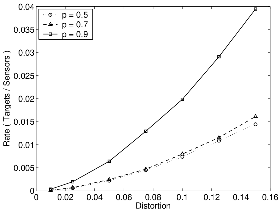
We compute the capacity bound $C_{LB}(D)$ for environments with probabilistic models of the form $P_{F}=[p\;(1-p)]$ and $P_{F|F^{\prime}}=[p\;(1-p);\;(1-p)\;p]$ where $p\in[0,1]$. In Figure 3, we demonstrate the effect of structure in the environment on $C_{LB}(D)$ by varying $p$. $p=0.5$ corresponds to an unstructured environment (all $\boldsymbol{f}$ equally likely), and increasing values of $p$ correspond to increasing spatial structure (e.g. increasing target sparsity). We assume that the sensors have range $c=0$ (i.e. they sense only one target) and that the sensing function $\Psi$ is the identity function. The sensor noise model assumes that the sensor’s output is flipped with probability $0.1$. Figure 3 demonstrates that $C_{LB}(D)$ increases for more structured environments (i.e. fewer sensors are needed as $p$ increases).

References

- [1] E. J. Duarte-Melo and M. Liu, “Data-gathering wireless sensor networks: organization and capacity,” Computer Networks: Special Issue on Wireless Sensor Networks, vol. 43, 2003.
- [2] A. Scaglione and S. D. Servetto, “On the interdependence of routing and data compression in multi-hop sensor networks,” in Proc. 8th ACM Int. Conference on Mobile Computing and Networking, Sept. 2002.
- [3] M. Gastpar and M. Vetterli, “Power-bandwidth-distortion scaling laws for sensor networks,” in Third. Int. Symp. Info. Proc. in Sensor Networks, Apr. 2004.
- [4] S.Z. Li, Markov Random Field Modeling in Image Analysis, Springer-Verlag, 2001.
- [5] Y. Rachlin, R. Negi, and P. Khosla, “Sensing capacity for target detection,” in Proc. IEEE Inform. Theory Wksp., Oct. 24-29 2004.
- [6] Y. Rachlin, R. Negi, and P. Khosla, “Sensing capacity for discrete sensor network applications,” in Proc. Fourth Int. Symp. on Inform. Proc. in Sensor Networks, April 25-27 2005.
- [7] P. Varshney, Distributed Detection and Data Fusion, Springer-Verlag, 1997.
- [8] K. Chakrabarty, S. S. Iyengar, H. Qi, and E. Cho, “Coding theory framework for target location in distributed sensor networks,” in Proc. Int. Conf. on Inform. Technology: Coding and Computing, April 2001.
- [9] R.G. Gallager, Information Theory and Reliable Communications, Wiley, 1968.
- [10] I. Csiszar, “The method of types,” IEEE Trans. Inform. Theory, vol. 44, no. 6, 1998.