Distributed Algorithms for Optimal Rate-Reliability Tradeoff in Networks
Abstract
The current framework of network utility maximization for distributed rate allocation assumes fixed channel code rates. However, by adapting the physical layer channel coding, different rate-reliability tradeoffs can be achieved on each link and for each end user. Consider a network where each user has a utility function that depends on both signal quality and data rate, and each link may provide a ‘fatter’ (‘thinner’) information ‘pipe’ by allowing a higher (lower) decoding error probability. We propose two distributed, pricing-based algorithms to attain optimal rate-reliability tradeoff, with an interpretation that each user provides its willingness to pay for reliability to the network and the network feeds back congestion prices to users. The proposed algorithms converge to a tradeoff point between rate and reliability, which is proved to be globally optimal for codes with sufficiently large codeword lengths and user utilities with sufficiently negative curvatures.
I Introduction
Since the publication of the seminal paper [1] by Kelly et al. in 1998, the framework of Network Utility Maximization (NUM) has found many applications in network rate allocation algorithms and Internet congestion control protocols, e.g., in [2, 3, 4, 5]. Consider a communication network, wireless or wired, with logical links, each with a fixed capacity of bps, and sources (i.e., end users), each transmitting at a source rate of bps. Each source emits one flow, using a fixed set of links in its path, and has a utility function . Each link is shared by a set of sources. NUM, in its basic version solved by a standard distributed algorithm, is the following problem of maximizing the total utility of the network , over the source rates , subject to linear flow constraints for all links :
| (1) |
A major limitation of formulation (1) is that physical layer opportunities are entirely ignored. On links where physical layer’s adaptive resource allocation can change the information ‘pipe’ sizes, e.g., through power control and adaptive coding, each link capacity is no longer a fixed constant but a function of resource allocation [6]. For example, changing the code rate on a link changes both the attainable throughput and decoding error probability on the link. A larger can be obtained on a link at the expense of lower decoding reliability, which in turn lowers the end-to-end signal quality for sources traversing the link and reduces user utilities at those sources if utilities depend on both rate and reliability. Dynamic adjustment of reliability provides an additional degree of freedom for improving each user’s utility as well as the system efficiency. For example, if we allow lower decoding reliability on more congested links and higher decoding reliability on less congested links, we may be able to improve end-to-end joint rate-reliability performance for all users. Such physical layer opportunities are to be leveraged in both wireless systems and wired networks such as DSL broadband access. However, the standard distributed algorithm based on congestion prices (e.g., [1, 4]) cannot be applied since the concept of noisy link and physical layer coding are absent from the basic NUM formulation (1).
In this paper, we exploit the tradeoff between information data rate and signal reliability attained for each source, by controlling the code rate, or equivalently, decoding error probability, for each source’s flow on each link and end-to-end information data rate of each sources’ flow. As in [6], we study a joint transport and physical layer problem in the context of ‘layering as optimization decomposition’. In contrast to [6], where power control is considered at the physical layer, in this paper, we consider reliability of each link through error control coding at the physical layer. The new optimization formulation we propose in general has coupled and nonconvex constraints. Two pricing-based distributed algorithms proposed converge to the globally optimal rate-reliability tradeoff under certain sufficient conditions. Two approaches will be examined: the integrated dynamic reliability policy, where a link provides the same error probability (i.e., the same code rate) to each of the sources whose flows traverse it, and the differentiated dynamic reliability policy, where a link can provide a different error probability (i.e., a different code rate) to each of the sources.
II System model
We assume that each source has a utility function , where is an information data rate and is reliability of received bits of an elastic traffic source . Similar to most models based on NUM, we assume that is a smooth, increasing, and strictly concave function of and . Information data rate for each source may be constrained within a range , and there may be a minimum reliability requirement . The reliability of source is defined as where is an end-to-end error probability for the flow from source . Each link has its maximum transmission capacity . After link receives the data of source from the upstream link, it first decodes it to extract the information data and encodes it again with its own code rate, , where code rate is defined as the ratio of the information data rate (bps) at the input of the encoder to the transmission data rate (bps) at the output of the encoder [7]. This allows the link to adjust both transmission rate and error probability, since the transmission rate of source at link can be defined as
and the error probability of source at link can be defined as a function of by
This function rarely has a closed-form analytic expression, and will be approximated through known bounds. The end-to-end error probability for each source is . Assuming small decoding error probability (i.e., ), we can approximate the end-to-end error probability of source as
Hence, the reliability of source can be written as
Since each link has its transmission capacity , the sum of transmission rates of sources that are traversing each link cannot exceed its transmission capacity, i.e.,
III Integrated dynamic reliability policy
We first investigate a more restrictive policy where a link provides the same code rate to each of the sources whose flows traverse it, i.e.,
and the NUM problem is formulated as
| (2) |
In order to derive a distributed algorithm to solve the above problem and to prove convergence to global optimum, the critical properties of separability and convexity of problem (2) need to be carefully examined. Because of the physical layer coding and rate-reliability tradeoff we introduced into the problem formulation, these two properties no longer trivially hold as in the basic NUM (1).
Integrated policy naturally leads to a decomposition of problem (2), since the second constraint can be written as
| (3) |
The more complicated issue is convexity of function . If random coding based on -ary binary coded signals is used, an upper bound on the error probability is [8]:
where is the block length and is the cutoff rate. Hence, if we take
it is a convex function for given and . A more general approach is to use the random code ensemble error exponent [7] that upper bounds the decoding error probability:
where is the codeword block length and is the error exponent function. In general, may not be convex, even though it is known [7] that is a convex function. The following lemma provides a sufficient condition for convexity of .
Lemma 1. If the absolute value of the first derivatives of is bounded away from 0 and the absolute value of the second derivative of is upper bounded, then for a large enough codeword block length , is convex.
Proof:
Assume that there exist positive constants and such that and .
Hence, for . ∎
Throughout this paper, we assume that the conditions in the above lemma are true and the channel code is strong enough, i.e., is large enough. In such cases, problem (2) is a convex and separable optimization problem, which can be solved by the following distributed algorithm where each source and each link solve their own problems only with local information and limited message passing. This distributed algorithm is derived by decomposing the dual problem of (2) (not shown explicitly in this summary), and we can interpret dual variables and as the price per unit rate to use link and the price per unit reliability that the source must pay to the network, respectively.
Algorithm 1.
In each iteration , by solving the following problem (4)11 1 Optimization problems (4) and (6) (also problems (11) and (13) in Algorithm 2) are convex optimization in only one or two variables with simple range constraints. Hence, they can be easily solved by using standard algorithms such as a gradient projection algorithm. over , each source determines its information data rate and desired reliability (i.e., and ) that maximize its net utility based on the prices in the current iteration. Furthermore, by price update equation (5), the source offers price per unit reliability for the next iteration.
Source problem and reliability price update at source :
| (4) |
where .
| (5) |
where and is step size, which can be taken as for some .
Concurrently in each iteration , by solving problem (6) over , each link determines its code rate (i.e., ) that maximizes the ‘net revenue’ of the network based on the prices in the current iteration. In addition, by price update equation (7), the link adjusts its congestion price per unit rate for the next iteration.
Link problem and congestion price update at link :
| (6) |
where .
| (7) |
where .
In the above Algorithm 1, source needs to know , the sum of ’s of links that are along its path . This can be obtained by the notification from the links e.g., through acknowledgment packets. To carry out price update (5), the source needs to know the sum of error probabilities of the links that are along its path (i.e., its own reliability that is provided by the network, ). This can be obtained by the notification from the links that determines the code rate for the source (by solving problem (6)) or obtained by the notification from the destination that measures the end-to-end reliability. To solve the link problem (6), each link needs to know , the sum of ’s from sources using this link . This can be obtained by the notification from these sources. To carry out update (7), the link needs to know the aggregate information data rate of the sources that are using it (i.e., ). This can be obtained by measuring it by the link itself.
With dual decomposition and Lemma 1, the following result can be proved using standard techniques in distributed gradient algorithm’s convergence proof:
Theorem 1. By Algorithm 1, dual variables and converge to the optimal dual solutions and and the corresponding primal variables , , and are the globally optimal primal solutions of (2).
IV Differentiated dynamic reliability policy
In this policy, a link may provide a different code rate to each of the sources traversing it. An example of practical code constructions that enable such a flexibility is the coding technique with embedded diversity recently proposed in [9], which allows data streams with different rate-reliability tradeoffs be embedded within each other.
The problem formulation in (2) needs to be generalized to the following:
| (8) |
The objective function and constraints of problem (8) are the same as those of problem (2) except that we have here instead of . Due to this critical difference, problem (8) in general is neither a convex problem nor a separable one (since we may not modify the second constraint in this problem as in (3)). To resolve this issue, we transform problem (8) by first introducing the auxiliary variables , which can be interpreted as the allocated transmission capacity to source at link . Then, the above problem can be reformulated as
| (9) |
The second constraint in problem (8) is now decomposed into two constraints in problem (9): the second and third constraints. Here, the second constraint implies that the transmission data rate of each source at each link must be smaller than or equal to its allocated transmission capacity at the link, and the third constraint implies that the aggregate allocated transmission capacity to the sources at each link must be smaller than or equal to its maximum transmission capacity. In this formulation, each link explicitly allocates a transmission capacity to each of its sources. We can easily show that problem (9) is equivalent to problem (8), since at optimality, the second constraint in problem (9) is satisfied with the equality.
The next step of problem transformation is to take a log change of variable at the second constraint in problem (9) and set (i.e., ). This reformulation turns problem (8) into the following equivalent problem:
| (10) |
where and and .
Note that problem (10) is separable but still may not be a convex optimization problem since the objective may not be a concave function, even though is a concave function. The following lemma provides a sufficient condition for its concavity. For notational simplicity, assume that is additive in each variable (the general case is an easy extension), (i.e., ), and be a strictly concave function of . Define
Lemma 2. If , is a concave function of and is a concave function of and .
Proof:
Since ,
Hence, if , is a concave function of ∎
The condition of is equivalent to:
Since utility functions are increasing, is a positive number. The above inequality states that the utility function needs to be not just concave (i.e., ), but with a curvature that is bounded away from 0 by as much as , i.e., the user utility function must be ‘elastic’ enough.
For example, consider the often-used utility functions [5]:
For this family of utility functions parameterized by , Lemma 2 shows that problem (10) becomes a convex optimization problem if .
After the above procedures of problem transformations, we are ready to provide a distributed algorithm based on dual decomposition to solve problem (10), and to prove the performance guarantee on global optimality provided that the conditions in Lemmas 1 and 2 hold.
Algorithm 2.
Equations (4)-(7) are now replaced by (11)-(14). In contrast to Algorithm 1 that does not keep per-flow information on the links, in the more complex Algorithm 2, each link differentiates each of the flows through it by providing a different code rate , a different congestion price , and an explicit capacity allocation . In addition, the congestion price is determined based on the allocated capacity and the transmission rate of each individual source that uses link in Algorithm 2, while the congestion price is determined based on the aggregate transmission rate of sources that use link and the transmission capacity of the link in Algorithm 1.
Source problem and reliability price update at source :
| (11) |
where .
| (12) |
where .
Link problem and congestion price update at link :
| (13) |
| (14) | |||||
Theorem 2. By Algorithm 2, dual variables and converge to the optimal dual solutions and and the corresponding primal variables , , , and are the globally optimal primal solutions of problem (10).
Extensions of Algorithms 1 and 2 to asynchronous version with constant step size can be carried out similar to those in [6].
V Numerical examples

We present numerical examples for a simple network shown in Figure 1. Utility function for user has the following standard form of concave utility:
where is a constant () that determines the relative weight between rate and reliability. The decoding error probability on each link is assumed to be the following form: where is the channel code block length and the code rate for link . We set , (Mbps), (Mbps), (Mbps), , and .
We trace the globally optimal tradeoff curve between rate and reliability, and also compare the total network utility achieved by the following three policies:
- •
Static reliability
- •
Integrated dynamic reliability
- •
Differentiated dynamic reliability.
In the static scheme, each link provides a fixed error probability 0.025 and rate is allocated to each user by solving the basic NUM problem (1).
We first investigate the case where all the users have the same , and vary the value of from 0 to 1 in step size of 0.1. The resulting tradeoff curve obtained by Algorithm 1, which is globally optimal, is shown in Figure 2. As expected, a larger (i.e., utility from rate given a heavier weight) leads to a higher rate at the expense of lower reliability. The more congested links a user’s flow passes through, the steeper the tradeoff curve becomes. For each user, the area to the left and below of the tradeoff curve is the achievable region, and the area to the right and above of the tradeoff curve is the infeasible region. It is impossible to operate in the infeasible region and inferior to operate in the interior of the achievable region. Operating on the boundary of the achievable region, i.e., the Pareto optimal tradeoff curve, is the best.

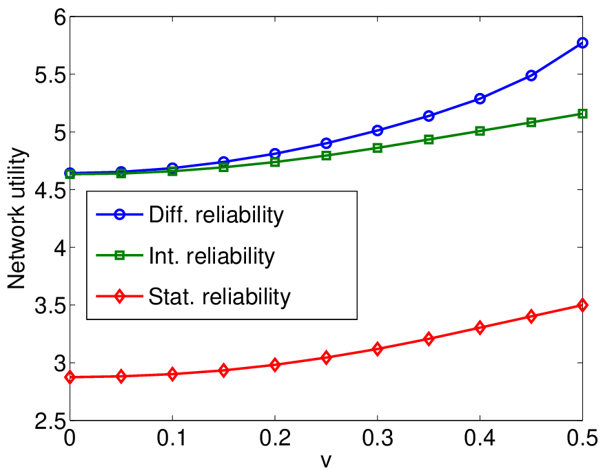
We then give different weights to the eight users:
and vary from 0 to 0.5 in step size of 0.05. Figure 3 shows the relative performance in terms of network utility achieved by the three policies as changes. The performance of Algorithms 1 and 2 that take into account rate-reliability tradeoff is significantly better than the standard distributed algorithm for the basic NUM (1) that ignores the possibility of jointly optimizing rate and reliability.
VI Concluding Remarks
Motivated by needs from the application layer and possibilities at the physical layer, this paper removes the rate-dependency assumption on utility functions in the current NUM formulation and allows the physical layer adaptive channel coding to tradeoff rate and reliability on each link and for all the sources. We present two distributed algorithms for two possible formulations of the problem, and provide the sufficient conditions on codeword length and utility curvature under which convergence to the globally optimal rate-reliability tradeoff can be proved. In addition to link-updated congestion prices for distributed rate control, we also introduce source-updated signal quality prices for distributed reliability control. The tradeoff between packet drop probability and traffic load may be investigated similar to that between decoding error probability and transmission rate examined in this paper.
References
- [1] F. P. Kelly, A. Maulloo, and D. Tan, “Rate control for communication networks: shadow prices, proportional fairness and stability,” Journal of Operations Research Society, vol. 49, no. 3, pp.237-252, March 1998.
- [2] S. Kunniyur and R. Srikant, “End-to-end congestion control: utility functions, random losses and ECN marks,” IEEE/ACM Trans. on Networking, vol. 11, no. 5, pp. 689-702, October 2003.
- [3] R. J. La and V. Anantharam, “Utility-based rate control in the Internet for elastic traffic,” IEEE/ACM Trans. on Networking, vol. 10, no. 2, pp. 272-286, April 2002.
- [4] S. H. Low, “A duality model of TCP and queue management algorithms,” IEEE/ACM Trans. on Networking, vol. 11, no. 4, pp. 525-536, August 2003.
- [5] J. Mo and J. Walrand, “Fair end-to-end window-based congestion control,” IEEE/ACM Trans. on Networking, vol. 8, no. 5, pp. 556–567, October 2000.
- [6] M. Chiang, “Balancing transport and physical layer in wireless multihop networks: Jointly optimal congestion control and power control,” IEEE J. Sel. Area Comm., vol. 23, no. 1, pp. 104–116, January 2005.
- [7] R. G. Gallager, Information Theory and Reliable Communication, Wiley, 1968.
- [8] J. G. Proakis, Digital Communications, McGraw-Hill, 1989.
- [9] A. R. Calderbank, S. N. Diggavi, and N. Al-Dhahir, “Space-time signalling based on Kerdock and Delsarte-Goethals codes,” Proc. IEEE ICC., Paris, France, June 2004.