Methods for Analytical Understanding of Agent-Based Modeling of Complex Systems
Abstract
Von Neuman’s work on universal machines and the hardware development have allowed the simulation of dynamical systems through a large set of interacting agents. This is a bottom-up approach which tries to derive global properties of a complex system through local interaction rules and agent behaviour. Traditionally, such systems are modeled and simulated through top-down methods based on differential equations. Agent-Based Modeling has the advantage of simplicity and low computational cost. However, unlike differential equations, there is no standard way to express agent behaviour. Besides, it is not clear how to analytically predict the results obtained by the simulation. Such observations got the attention of the scientific community and some techniques have been proposed in order to cover these gaps in the agent-based modeling field. In this paper we survey some of these methods. For expressing agent behaviour formal methods, like Stochastic Process Algebras have been used. Such approach is useful if the global properties of interest can be expressed as a function of stochastic time series. However, if space variables must be considered, that means, if the space distribution of agents is important we shall change the focus. In this case, multiscale techniques, based on Chapman-Enskog expansion was used to establish the connection between the microscopic dynamics (agent behaviour) and the macroscopic observables. Besides, knowledge discovery in agent systems is a NP problem. This is the motivation for using data mining techniques, like Principal Component Analysis (PCA), to study agent systems like Cellular Automata. With the help of these tools (Stochastic Process Algebras, Chapman-Enskog expansion and PCA) we will discuss a simple society model, a Lattice Gas Automaton for fluid modeling, and knowledge discovery in CA databases. Besides, we show the capabilities of the NetLogo, a free software for agent simulation of complex system and describe our experience with this package.
1 . Introduction
With the development of the hardware the possibility of simulating a system by constructing a mathematical model and executing it on a computer has opened new frontiers in science and engineer [22, 31, 10, 30]. Traditionally, the mathematical model is based on differential equations connecting the macroscopic variables that define the system [22, 31]. For example, the majority of the fluid models follow the Eulerian formulation of fluid mechanics; that is, the fluid is considered as a continuous system subjected to Newton’s and conservation Laws as well as state equations connecting the thermodynamic variables of pressure , density and temperature [22]. This is a top-down approach which attempts to capture the nature of the relationships between macroscopic variables without been specific about the essence of the microscopic scales.
On the other hand, agent-based modeling tries to emulate the system behavior following another viewpoint [2, 30]. In this case, the model consists of a set of agents that encapsulate the behaviors of the individuals that make up the system, and execution consists of emulating these behaviors [7, 3, 21]. These are bottom-up models based on the description of the individuals (agents) and their local interactions as well as the belief that the macroscopic observables and their relationships can be derived from the microscopic (agents) interactions. For instance, that is the philosophy behind Lattice Gas Cellular Automata models for fluids [11] as well as some techniques for simulating social and ecological processes [3].
In this paper we focus on agent-based models for natural phenomena. We observe two approaches in this field: Cellular Automata and Agent-Based Cellular Automata approaches. Cellular Automata are discrete and finite dynamical systems that evolve following simple and local rules which can be deterministic of probabilistic ones. For example, in modeling pheromone trails [32], each cell might contain a pair of state values as well as the amount of pheromone at a certain position and a binary value determining whether or not an ant is present in that cell. If a cell contains an ant then it will move to the adjoining cell with the most pheromone, depositing pheromone in the cell it leaves. Otherwise, the pheromone in a cell without an ant will decrease (due to evaporation).
Instead of expressing the rules of the above model in terms of update rules for cells, the rules could be equally well expressed in terms of how each ant behaves, that is, an algorithm is used to describe the behavior of the ant and if it moves between cells, on each time step choosing the neighbouring cell with the most pheromone. In this viewpoint, the agent-base one, we can abstract the space distribution of agents and focus in their activities and interactions. Obviously, space distributions are easily recovered by imposing that ants move on a lattice. So agent based modeling incorporates the cellular automata philosophy also.
Agent-Based Modeling, has the advantage of simplicity and low computational cost. However, unlike differential equations, there is no standard way to express agent behavior. Besides, it is not clear how to analytically predict the results obtained by the simulation.
This paper is organized as follows. The next section presents the basic concepts of CAs and how computational intractable problems arise in this area. Then, Section 3 shows the application of PCA for cellular automata analysis. In Section 5 we review the WSCCS, a stochastic process algebra, and its application for expressing agent behavior and interaction. Section 6 presents the Chapman-Enskog expansion in the context of cellular automata for fluid modeling. In Section 7 we describe the NetLog capabilities and present our implementation of the HPP through NetLog tools. Finally, we discuss some perspectives in the field of agent-based modeling and simulation.
2 . Cellular Automata
A cellular automaton (CA) is a quadruple where is a set of indices or sites, is the finite set of site values or states, is a one-to-many mapping defining the neighborhood of every site as a collection of sites, and is the evolution function of [38, 5]. The neighborhood of site is defined as the set ( stands for the integer part of ). Note that a given site may or not be included in its own neighborhood. Since the set of states is finite, will denote the set of possible rules of the CA taken among the rules.
For a one-dimensional cellular automaton the lattice is an array of sites, and the transition rule updates a site value according to the values of a neighborhood of sites around it, that means:
| (1) |
| (2) | |||||
| (3) |
where means the evolution time, also taking discrete values, and means the value of the site at time [38, 4] (see also [36] for on-line examples). Therefore, given a configuration of site values at time , it will be updated through the application of the transition rule to generate the new configuration at time , and so on. In the case of in Expression (2) and we have a special class of cellular automata which was widely studied in the CA literature [29, 12, 9, 38]. Figure 1 shows the very known example of such a CA. The rule in this case is:
| (4) |
that means, the remainder of the division by two. The figure pictures the evolution of an initial configuration in which there is only one site with the value .

Once in Expression (2), it is easy to check that this rule is defined by the function:
| (5) |
| (6) |
By observing this example, we see that there are such rules and for each one it can be assigned a rule number following the indexation illustrated on Expression (6). In [37], Wolfram proposes four basic classes of behavior for these rules (see also [5]):
Class 1: Evolution leads to homogeneous state in which all the sites have the same value (Figure 2.a);
Class 2: Evolution leads to a set of stable and periodic structures that are separated and simple (Figure 2.b);
Class 3: Evolution leads to a chaotic pattern (Figure 2.c);
Class 3: Evolution leads to complex structures (Figure 2.d).

(a)

(b)

(c)

(d)
Other classifications based on Markovian processes and group properties can be also found in the literature [20, 13].
Despite of its local simplicity, knowledge discovery in CA is a NP problem. In fact, let us take a one-dimensional CA with a finite lattice of size . One may consider the question of whether a particular sequence of site values can occur after time steps in the evolution of the cellular automaton, starting from any initial state. Then, one may ask whether there exists any algorithm that can determine the answer in a time given by some polynomial in and . The question can certainly be answered by testing all sequences of possible initial site values, that is . But this procedure requires a time that grows exponentially with .
Nevertheless, if an initial sequence could be guessed, then it could be tested in a time polynomial in and . As a consequence, the problem is in the class NP which motivates the application of data mining techniques for knowledge discovery in CA. The next sections review PCA basic theory and its application for the analysis of the (traditional) set of rules composed by cellular automata obtained when , .
3 . Principal Component Analysis
Principal Component Analysis (PCA), also called Karhunen-Loeve, or KL method, can be seen as a method for data compression or dimensionality reduction [6] (see [24], section also). Thus, let us suppose that the data to be compressed consist of tuples or data vectors, from a n-dimensional space. Then, PCA searches for n-dimensional orthonormal vectors that can best be used to represent the data, where . Figure 3.a-b pictures this idea using a bidimensional representation. If we suppose the data points are distributed over the ellipse, it follows that the coordinate system ( shown in Figure 3.b) is more suitable for representing the data set in a sense that will be formally described next.
Thus, let be the data set represented on Figure 3. By now, let us suppose that the centroid of the data set is the center of the coordinate system, that means:
| (7) |
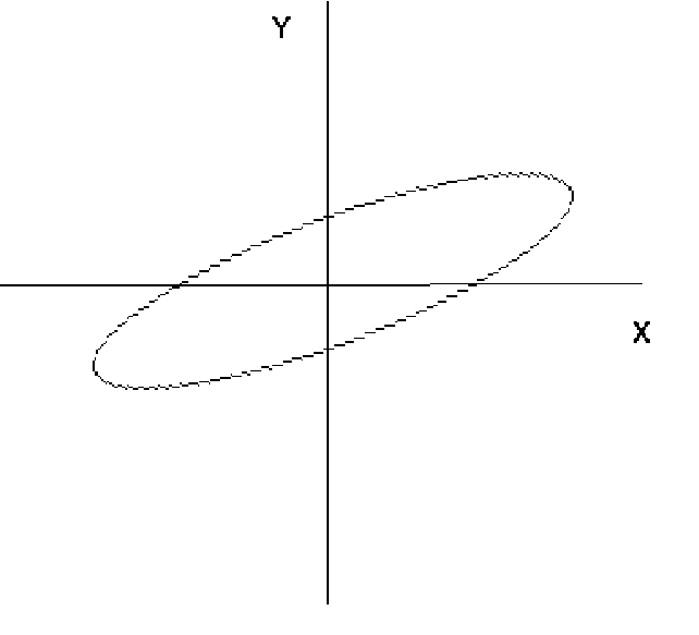
(a)

(b)
To address the issue of compression, we need a vector basis that satisfies a proper optimization criterion (rotated axes in Figure 3.b). Following [24], consider the operations in Figure 4. The vector is first transformed to a vector by the matrix (transformation) . Thus, we truncate by choosing the first elements of . The obtained vector is just the transformation of by , that is a matrix with 1s along the first diagonal elements and zeros elsewhere. Finally, is transformed to by the matrix . Let the square error defined as follows:
| (8) |
where means the trace of the matrix between the square brackets and the notation () means the transpose of the complex conjugate of a matrix. Following Figure 4, we observe that . Thus we can rewrite (8) as:

| (9) |
which yields:
| (10) |
where:
| (11) |
Following the literature, we call the covariance matrix. We can now stating the optimization problem by saying that we want to find out the matrices that minimizes . The next theorem gives the solution for this problem.
Theorem 1: The error in expression (10) is minimum when
| (12) |
where is the matrix obtained by the orthonormalized eigenvectors of arranged according to the decreasing order of its eigenvalues.
Proof. To minimize we first observe that must be zero if Thus, the only possibility would be
| (13) |
Besides, by remembering that
| (14) |
we can also write:
| (15) |
Again, this expression must be null if . Thus:
This error is minimum if:
| (16) |
that is, if and are unitary matrix. The next condition comes from the differentiation of respect to the elements of . We should set the result to zero in order to obtain the necessary condition to minimize . This yields:
| (17) |
which renders:
| (18) |
By using the property (14), the last expression can be rewritten as
Since is fixed, will be minimized if
| (19) |
is maximized where is the ith row of . Once is unitary, we must impose the constrain:
| (20) |
Thus, we shall maximize subjected to the last condition. The Lagrangian has the form:
where the are the Lagrangian multipliers. By differentiating this expression respect to we get:
| (21) |
Thus, are orthonormalized eigenvectors of . Substituting this result in expression (19) produces:
| (22) |
which is maximized if correspond to the largest eigenvalues of . ()
A straightforward variation of the above statement is obtained if we have a random vector with zero mean. In this case, the pipeline of Figure 4 yields a random vector and the square error can be expressed as:
which can be written as:
| (23) |
where is the covariance matrix. Besides, if in Expression (7) is not zero, we must translate the coordinate system to before computing the matrix , that is:
| (24) |
In this case, matrix will be given by:
Also, sometimes may be useful to consider in Expression (8) some other norm, not necessarily the 2-norm. In this case, there will be a real, symmetric and positive-defined matrix , that defines the norm. Thus, the square error will be rewritten in more general form:
| (25) |
Obviously, if we recover Expression (8). The link between this case and the above one is easily obtained by observing that there is non-singular and real matrix , such that:
| (26) |
The matrix defines the transformation:
| (27) |
Thus, by inserting these expressions in Equation (25) we obtain:
| (28) |
Expression (28) can be written as:
| (29) |
now using the 2-norm, like in Expression (8). Therefore:
| (30) |
Following the same development performed above, we will find that we must solve the equation:
| (31) |
where:
| (32) |
Thus, from transformations (27) it follows that:
| (33) |
and, therefore, we must solve the following eigenvalue/eigenvector problem:
| (34) |
The eigenvectors, in the original coordinate system, are finally given by:
| (35) |
The next section shows the application of PCA method for knowledge discovery in CAs.
4 . PCA and Cellular Automata
In this section we review the work presented in [14]. In this reference, the authors analyzed one-dimensional CAs using PCA. The key idea is to consider binary patterns of a pre-defined size as inputs of the CAs. It is considered the one-dimensional CA rules obtained for and in expression 1-2. The output can be collected in a Table, like Table 1, built for .
| Patterns | … | ||||
| … | |||||
| … | |||||
| … | … | … | … | … | … |
| … | |||||
| … |
Each row of Table 1 is obtained through the application of the rule (see Expression (6) for an example of rule indexation) Then, I/O patterns are converted to cardinal numbers denoted by , which means the cardinal number corresponding to the application of the rule to the pattern ( for Table 1). Thus, in general, we get the matrix:
| (36) |
where The matrix is the data set to be analyzed.
For mining knowledge in through PCA we should firstly to perform the operation (translation) given by (24). Thus, matrix is converted to the following one:
| (37) |
with:
| (38) |
| (39) |
The matrix is of size . In [14] columns of are called variables while rows are called covariables. However, we must observe that space dimension is the number of rules and the number of data vectors is the number of patterns . Thus, following Section 3, we should apply the PCA over the data set given by matrix in order to find out the principal components of the covariables space. Besides, in [14] the norm of the covariables space is defined by:
| (40) |
with:
| (41) |
Following Section 3, we must solve Equation (34) to find the eigenvalues and then apply Expression (35) to get the eigenvectors in the desired representation. The Table 2 shows the larger eigenvalues of this matrix for the listed pattern sizes.
| l | |||||||
|---|---|---|---|---|---|---|---|
| 4 | 52.6802 | 48.2214 | 36.8869 | 36.8263 | 36.3134 | 24.4539 | 18.6179 |
| 5 | 58.2575 | 50.9776 | 37.2301 | 37.0399 | 30.7382 | 21.7355 | 18.0214 |
| 6 | 59.5952 | 51.6519 | 37.3406 | 37.1109 | 29.3769 | 21.0940 | 17.8305 |
| 7 | 59.9260 | 51.8197 | 37.3696 | 37.1296 | 29.0383 | 20.9358 | 17.7811 |
| 9 | 60.0290 | 51.8721 | 37.3788 | 37.1355 | 28.9325 | 20.8865 | 17.7656 |
| 12 | 60.0358 | 51.8755 | 37.3794 | 37.1359 | 28.9256 | 20.8833 | 17.7645 |
The main result is that the eigenvalues from the seventh rank are dramatically smaller in magnitude ( times) than the first seven ones. Such observation led authors of [14] towards the following conjecture:
Conjecture: The rank of is and does not depend on the size of patterns being considered. When is increased the eigenvalues tend to characteristic values obtained for
This is the main result presented in [14]. Next, we show our results by applying the same analysis but introducing randomness in the CA behavior.
5 . Stochastic Process Algebra and Agents
If we can break down a system into component parts that act as finite state machines, then we can apply formal methods to explain how they are combined to form the observed (macroscopic) whole. That is the key idea of using process algebra for modeling societies [21, 30]. Process algebra are widely used in the analysis of distributed computer systems [1]. They allow formal reasoning about how the various components of a system contribute to its overall behavior [26, 23].
In [32], it is argued that a stochastic process algebras, the Weighted Synchronous Calculus of Communicating Systems (WSCCS), provides a useful formalism for understanding the dynamical behavior of their colony, since they combine computer simulation, Markov chain analysis and mean-field methods of analysis. Next, we review the basic elements of a process algebra and show its application for modeling societies.
5.1 . Stochastic Process Algebra
One of the best known process algebra, and also a remarkable one in this area, is the Calculus of Communicating Systems (CCS) [1]. It uses the notions of agents (or processes) and actions. Agents describe the entities which make up a system, such as processes in a distributed system, and actions that allow the agents communication (interaction). These notions are formally described which permits logical reasoning about the system [8]. Besides, in [1] a new equivalence concept for agents, which are finite state automata, is provided. The CCS makes no attempt to actions synchronization and priority. The WSCCS adds such features to the CCS [33, 34, 35].
Any process algebra consists of essentially four components [8]:
1. A syntax for describing agents (automata) and the actions they perform.
2. Algebraic rules.
3. Derivation rules.
4. A congruence for defining when two automata are considered equivalent
in all algebraic contexts.
5. An equational theory which defines how the equivalence of automata is demonstrated from the syntax of the agents which compose them.
For instance, in the WSCCS it is used the following syntax:
Agents are labeled by capital letters like .
The set of allowed actions form an abelian group , where is the group operation. The identity action, denoted by , can be seen as a tick of a global clock. Each time a occurs time has just moved forward one step. The inverse of an action is denoted by , which means, . This operation will formally represent communication between agents in the WSCCS.
For example, let us suppose that we have two agents and and that, in a single unit of time, there is a probability that becomes and a probability that it remains unchanged. Thus, we can define by the following algebraic expression in WSCCS:
| (42) |
where the indicates that the agent can make a choice. In Expression (42), each possible choice will define a transition and the transitions will define the derivation rules. Formally, we write:
| (43) |
| (44) |
In general, we have:
| (45) |
which means that agent may change to , with probability , when action occurs.
Another important operation is the composition of agents. Given the agents and , where are possible actions, their composition is formally defined by:
| (46) |
This expression do not incorporates the probability. The following expression adds this feature:
| (47) |
where is the probability of agent (the same for and ).
Expressions (46)-(47) are simple examples of equational laws of WSCCS. A complete development can be found in [33, 35]. However, our simple presentation allows to point out the power of WSCCS for society modeling. Hence, let us consider the simple example of a colony of ants (agents) that can be only or . In this example, described in [32], the active agent is defined by an expression analogous to Equation (42):
| (48) |
The passive agent works differently. Following [32], we assume that it remains passive forever, thus:
| (49) |
The natural question now is: How to combine ants in order to define a colony? This question is answered by the composition operation (Expressions (46),(47)). Henceforth, we write a colony of ants, of which are Active agents, as:
| (50) |
| (51) |
We shall obtain the meaning of the coefficients:
| (52) |
Firstly, according to Equation (45), the transitions are given by:
| (53) |
In order to interpret , we consider now the sequence of random variables where for each , that represent the outcome of a series of transitions on the agent with initial state consisting of all ants in the active state. We can think as the number of ticks of a global clock. From expression (51) it is straightforward to observe that:
| (54) |
¿From this expression, we observe the WSCCS model, given by Equation (51), has underlying discrete time Markov chain. A Markov chain is a time ordered sequence of random variables where the variable of the sequence is conditional only on the variable ’s value [19]. In fact, this happens for WSCCS models in general (see Appendix A of [32]). Such feature is used in [32] in the context of ant societies. Basically, the transition rules can demonstrate properties that can help the analysis of important behaviors (asymptotic ones, for instance).
6 . Lattice Gas Automata and Multiscale Analysis
The WSCCS is useful for modeling and analysis of the discrete dynamics of agent system. The analysis does not attempt to get spatial distribution of observables. Such goal can be achieved by multiscale techniques. In this section we consider the FHP model, which is a Lattice Gas Cellular Automata model, used for fluid simulation. Thus, space variables must be considered, that means. In this case, a multiscale technique based on Chapman-Enskog [25] expansion is used to establish the connection between the microscopic dynamics and the macroscopic observables.
The Chapman-Enskog method works as follows. Given an operator and the equation:
| (55) |
let us suppose that:
- 1.
The solution can be expressed as:
(56) - 2.
When this series is introduced in Expression (55) the result can be expressed as:
(57) - 3.
The functions are such that:
(58) (59) (60) (61)
which together ensure that Expression (55) is satisfied.
Therefore, following items (1)-(3) we say that the sub-series , , , , are successive approximations of Arbitrary elements may enter into the solution of Equations (57)-(61) as well as in the definition of the approximations and of the expansion (56). An interesting example is given by the FHP model.
The FHP was introduced by Frisch, Hasslacher and Pomeau [17] in 1986 and is a model of a two-dimensional fluid and it is an abstraction, at a microscopic scale, of a fluid. The FHP model describes the motion of particles traveling in a discrete space and colliding with each other. The space is discretized in a hexagonal lattice.
The microdynamics of FHP is given in terms of Boolean variables describing the occupation numbers at each site of the lattice and at each time step (i.e. the presence or the absence of a fluid particle). The FHP particles move in discrete time steps, with a velocity of constant modulus, pointing along one of the six directions of the lattice. The dynamics is such that no more than one particle enters the same site at the same time with the same velocity. This restriction is the exclusion principle; it ensures that six Boolean variables at each lattice site are always enough to represent the microdynamics.
In the absence of collisions, the particles would move in straight lines, along the direction specified by their velocity vector. The velocity modulus is such that, in a time step, each particle travels one lattice spacing and reaches a nearest-neighbor site.
In order to conserve the number of particles and the momentum during each interaction, only a few configurations lead to a non-trivial collision (i.e. a collision in which the directions of motion have changed). When exactly two particles enter the same site with opposite velocities, both of them are deflected by 60 degrees so that the output of the collision is still a zero momentum configuration with two particles. When exactly three particles collide with an angle of degrees between each other, they bounce back to where they come from (so that the momentum after the collision is zero, as it was before the collision). Both two- and three-body collisions are necessary to avoid extra conservation laws. Several variants of the FHP model exist in the literature [10, 15], including some with rest particles like models FHP-II and FHP-III.
For all other configurations no collision occurs and the particles go through as if they were transparent to each other.
The full microdynamics of the FHP model can be expressed by evolution equations for the occupation numbers defined as the number, , of particle entering site at time with a velocity pointing along direction , where labels the six lattice directions. The numbers can be or .
We also define the time step as and the lattice spacing as . Thus, the six possible velocities of the particles are related to their directions of motion by
| (62) |
Without interactions between particles, the evolution equations for the would be given by
| (63) |
which express that a particle entering site with velocity along will continue in a straight line so that, at next time step, it will enter site with the same direction of motion. However, due to collisions, a particle can be removed from its original direction or another one can be deflected into direction .
For instance, if only and are at site , a collision occurs and the particle traveling with velocity will then move with either velocity or , where . The quantity
| (64) |
indicates, when that such a collision will take place. Therefore is the number of particles left in direction due to a two-particle collision along this direction.
Now, when , a new particle can appear in direction , as the result of a collision between and or a collision between e . It is convenient to introduce a random Boolean variable , which decides whether the particles are deflected to the right () or to the left (), when a two-body collision takes place. Therefore, the number of particle created in direction is
| (65) |
Particles can also be deflected into (or removed from) direction because of a three-body collision. The quantity which express the occurrence of a three-body collision with particles , and is
| (66) |
As before, the result of a three-body collision is to modify the number of particles in direction as
| (67) |
Thus, according to our collision rules, the microdynamics of a LGCA is written as
| (68) |
where is called the collision term.
For the FHP model, is defined so as to reproduce the collisions, that is
| (69) |
Using the full expression for and , given by the Equations (64)-(66), we obtain,
| (70) | ||||
These equations are easy to code in a computer and yield a fast and exact implementation of the model
Until now, we deal with microscopic quantities. However, the physical quantities of interest are not so much the Boolean variables but macroscopic quantities or average values, such as, for instance, the average density of particles and the average velocity field at each point of the system. Theses quantities are defined from the ensemble average of the microscopic occupation variables. Note that, is also the probability of having a particle entering the site , at time , with velocity
In general, a LGCA is characterized by the number of lattice directions and the spatial dimensionality . In our case and . Following the usual definition of statistical mechanics, the local density of particles is the sum of the average number of particles traveling along, each direction
| (71) |
Similarly, the particle current, which is the density times the velocity field , is expressed by.
| (72) |
Another quantity which will play an important role in the up coming derivation is the momentum tensor defined as
| (73) |
where the Greek indices and label the spatial components of the vectors. The quantity represents the flux of the component of momentum transported along the axis. This term will contain the pressure contribution and the effects of viscosity.
The starting point to obtain the macroscopic behavior of the CA fluid is to derive an equation for the . Averaging the microdynamics (68) yields
| (74) |
where is the collision term of the LGCA, under study. It is important to notice that has some generic properties, namely
| (75) |
expressing the fact that particle number and momentum are conserved during the collision process (the incoming sum of mass or momentum equals the outgoing sum).
The ’s vary between and and, at a scale e , one can expect them to be smooth functions of the space and time coordinates. Therefore, Equation (74) can be Taylor expanded up to second order and gives
| (76) | ||||
where is the second derivative in respect to the time parameter .
At a macroscopic scale , following the procedure of the so-called multiscale expansion [28], we introduce a new space variable such that
| (77) |
with . We also introduce the extra time variables and , as well as new functions depending on , and , and substitute into Equation (76)
| (78) |
together with the corresponding expressions for the second order derivatives. Then obtain new equations for the new functions . Thus, following step (1) above we may write [28] (see Expression (56)),
| (79) |
The Chapman-Enskog method is the standard procedure used in statistical mechanics to solve an Equation like (76) with a perturbation parameter . Assuming that can be factorized into , we write the contributions of each order in . According to multiscale Expansion (79), the right-hand side of (76) reads
| (80) |
Using Expressions (77)-(79) in the left-hand side of (76) and comparing the terms of the same order in in the Equation (80), yields
| (81) |
and
| (82) | ||||
where the subscript in spatial derivatives (e.g. ) indicates a differential operator expressed in the variable and , from Equation (62).
We also impose the extra conditions that the macroscopic quantities and are entirely given by the zero order of Expansion (79)
| (83) |
and therefore
| (84) |
Thus, following the Chapman-Enskog method we can obtain [16, 10], from Equation (76), the following result at order
| (85) |
and
| (86) |
On the other hand, if we considered the terms of order and using the Relations (85) and (86) to simplify, we have
| (87) |
The last equation contains the dissipative contributions to the Euler Equation (86). The first contribution is which is the dissipative part of the momentum tensor. The second part, namely comes from the second order terms of the Taylor expansion of the discrete Boltzmann equation. These terms account for the discreteness of the lattice and have no counterpart in standard hydrodynamics. As we shall see, they will lead to the so-called lattice viscosity. The order e can be grouped together to give the general equations governing our system. Summing Equations (85) and (87) with the appropriate power of as factor and we obtain
| (88) |
Similarly, Equation (86) and (87) yields [16]
| (89) |
We now turn to the problem of solving Equation (81) together with conditions (83) in order to find as functions of and . The solutions which make the collision term vanish are known as the local equilibrium solutions. Physically, they correspond to a situation where the rate of each type of collision equilibrates. Since the collision time is much smaller than the macroscopic observation time, it is reasonable to expect, in first approximation that an equilibrium is reached locally.
Provided that the collision behaves reasonably, it is found [16] that the generic solution is
| (90) |
This expression has the form of a Fermi-Dirac distribution. This is a consequence of the exclusion principle we have imposed in the cellular automata rule (no more than one particle per site and direction). This form is explicitly obtained for the FHP model by assuming that the rate of direct and inverse collisions are equal. The quantities e are functions of the density and the velocity field and are to be determined according to Equations (83). In order to carry out this calculation, is Taylor expanded up to second order in the velocity field . One obtains [10]
| (91) |
where are summed over the spacial coordinates, e.g. , , , and
| (92) |
The function is obtained from the fact that is the Taylor expansion of a Fermi-Dirac distribution. For FHP, it is found [10, 16]
We may now compute the local equilibrium part of the momentum tensor, and then obtain the pressure term
| (93) |
where .
We can see [16] that the lattice viscosity is given by
The usual contribution to viscosity is due to the collision between the fluid particles and is given by [16]
where is given by where
Therefore, the Navier-Stokes equation reads
| (94) |
where
| (95) |
is the kinematic viscosity of our discrete fluid.
Therefore, we demonstrated that the Navier-Stokes model can be reproduced by FHP technique. However, there is no need to solve Partial Differential Equations (PDEs) to obtain a high level of description. Such advantage can be explored in technological and scientific applications. For instance, in [18] we propose to combine the advantage of the low computational cost of LGCA and its ability to mimic the realistic fluid dynamics to develop a new animating framework for computer graphics applications.
7 . Tool for Agent-Based Simulation
Agent-based models can be analyzed by computer simulations. The NetLogo software is one possibility in this area [27]. It is a programmable modeling environment for simulating complex systems developing over time. Modelers can give instructions to hundreds or thousands of independent “ agents” all operating concurrently in order to explore the connection between the behavior of individuals and the macroscopic patterns that emerge from the interaction of many individuals. Users can create their own models using NetLogo facilities and documentations. It also comes with a Library of pre-written simulations that can be used and modified.
As an example of the NetLogo capabilities we describe our implementation of a Lattice Gas model called HPP [11]. It is similar to the FHP model described on Section 6 but, in this case, the lattice is a rectangular one. Figure 5 shows the NetLogo main interface and a snapshot of our HPP implementation.

The rules used for collision are explained in Figure 6. In the other situations the particles are considered transparent to each other when they cross the same site. There is also an exclusion principle: it is not allowed more than particle entering a given site with a given direction of motion. The aim of these rules is to reproduce some aspect of the real interactions between particles, namely that momentum and particle number are conserved during a collision. With such simple dynamics, we can model and simulate a gas of colliding particles and to obtain complex behaviors [11].
The HPP model is a kind of cellular automaton which has a lattice of sites that may have or crossing particles at a time . The rules define the system (particles) evolution and, consequently, the update of each site value.
The evolution of the sites is often split in two steps: collision and motion (or propagation). The collision phase solves interactions (collisions) through the rules pictured on Figure 6. During the propagation phase, the particles actually move to the nearest neighbor site they are traveling to.

(a)

(b)

(c)

(d)
The implementation the HPP in the NetLogo software we must define the agents, which are represented by arrows in the Figure 6, and the lattice. In the NetLogo system, the “ bricks” to compose an application are:
- 1.
Application Control: Button, Slider, Switch, Chooser.
- 2.
Plot.
- 3.
Monitor, Output and Text.
- 4.
Turtles: agents plus their graphical representation.
The Figure 5 shows the instances of some of these tools in our HPP implementation. The basic controls for the model are the following Buttons: (a) SETUP - Sets up screen with a given percentage of particles; (b) Execute - Run the model; (c) MOVE TURTLES- For move the particles with the mouse. There is one Slider to set the number of particles.
Behind the graphical interface for visualization and control the application, there is a code that implements agents behaviors. For example, let us consider the following code line:
| (96) |
if: Reporter must report a boolean (true or false) value.
any?: Reports true if the given agentset is non-empty, false otherwise.
other-BREED-here: Reports an agentset consisting of all turtles on the calling turtle’s patch (not including the caller itself). If a breed (a built-in turtle variable) is specified, like arrows in the above example, only turtles with the given breed are included.
heading: It is command in the NetLogo syntax. Each turtle picks a random integer between 0 and 359. Then the turtle sets its heading to the number it picked. Heading is measured in degrees, clockwise around the circle, starting with 0 degrees at twelve o’clock (north).
myself: It means “ the turtle or patch who asked me to do what I’m doing right now”.
who?: This is a built-in turtle variable. It holds the turtle’s id number (an integer greater than or equal to zero). You cannot set this variable; a turtle’s id number never changes. When NetLogo starts, or after you use the clear-all or clear-turtles commands, new turtles are created with ids in order, starting at 0. If a turtle dies, though, a new turtle may eventually be assigned the same id number that was used by the dead turtle.
jump: This is another command. Turtles move forward by number units all at once, without the amount of time passing depending on the distance.
NetLogo system has a lot of examples and a good documentation to help new users to write its own applications.
8 . Conclusions
The simulation of dynamical systems through a large set of interacting agents is an interesting research field with applications in areas like, physics, economy and sociology. This is a bottom-ut approach which tries to derive global properties of a complex system through local interaction rules and agent behavior. Agent-Based Modeling has the advantage of simplicity and low computational cost if compared with the traditional differential equation approaches.
In this paper we survey a method based on the WSCCS to express agent behavior which allow to analytically predict the results obtained by the simulation. Also, multiscale techniques, based on Chapman-Enskog expansion was reviewed to establish the connection between the microscopic dynamics (agent behavior) and the macroscopic observables. Besides, Principal Component Analysis (PCA) was analyzed for knowledge discovery in a Cellular Automata database. Finally, we show the capabilities of the NetLogo, a free software for agent simulation of complex system and describe our experience with this package. Our research will continue in this field, specially exploring the application of agent-based models for computer graphics applications.
9 . Acknowledgments
We would like to acknowledge CNPq, the Brazilian organization for scientific development, FAPERJ and the PCI-LNCC for the financial support for this work.
References
- [1] A Calculus of Communicating Systems, volume 92 of Lecture Notes in Computer Science. Springer-Verlag, 1980.
- [2] Agent-Based Modeling vs. Equation-Based Modeling: A Case Study and Users’ Guide., volume 1534 of Lecture Notes in Computer Science. Springer, 1998.
- [3] Integrating Geographic Information Systems and agent-based modeling techniques for simulating social and ecological processes. Oxford University Press, 2002.
- [4] A new kind of science. Wolfram Media Inc., Champaign, Ilinois, US, United States, 2002.
- [5] C. Adami. Introduction to Artificial Life. Springer, New York, 1998.
- [6] V. Algazi and D. Sakrison. On the optimality of karhunen-loeve expansion. IEEE Trans. Information Theory, pages 319–321, 1969.
- [7] R. Axelrod. The Complexity of Cooperation. Princeton University Press, 1997.
- [8] J. C. M. Baeten. A brief history of process algebra. Theor. Comput. Sci., 335(2-3):131–146, 2005.
- [9] P. Chaudhuri, D. Chowdhury, S. Nandi, and S. Chatterjee. Additive Cellular Automata, Theory and Applications, volume 1. IEEE Computer Society Press, Los Alamitos, California, 1997.
- [10] B. Chopard and M. Droz. Cellular Automata Modeling of Physical Systems. Cambridge University Press, 1998.
- [11] B. Chopard, A. Dupuis, A. Masselot, and P. Luthi. Cellular automata and lattice boltzmann techniques: An approach to model and simulate complex systems. Advances in complex systems, 5(2):1–144, 2002. special issue on: Applications of Cellular Automata in Complex Systems.
- [12] A. K. Das and P. P. Chaudhuri. Vector space theoretic analysis of additive cellular automata and its application for pseudoexhaustive test pattern generation. IEEE Trans. Comput., 42(3):340–352, 1993.
- [13] A. K. Das, A. Sanyal, and P. Palchaudhuri. On characterization of cellular automata with matrix algebra. Inf. Sci., 61(3):251–277, 1992.
- [14] L. Deniau and J. Blanc-Talon. PCA and cellular automata: a statistical approach for determnistic machines. 1994.
- [15] K. Diemer, K. Hunt, S. Chen, T. Shimomura, and G. Doolen. Density and velocity dependence of reynolds numbers for several lattice gas models. In G. Doolen, editor, Lattice Gas Methods for Partial Differential Equations, pages 137–177. Addison-Wesley, 1990.
- [16] U. Frisch, D. d’Humières, B. Hasslacher, P. Lallemand, Y. Pomeau, and J.-P. Rivet. Lattice gas hydrodynamics in two and three dimension. Complex Systems, 1:649–707, 1987. Reprinted in Lattice Gas Methods for Partial Differential Equations, ed. G. Doolen, p.77, Addison-Wesley, 1990.
- [17] U. Frisch, B. Hasslacher, and Y. Pomeau. Lattice-gas automata for the Navier-Stokes equation. Phys. Rev. Lett., 56:1505, 1986.
- [18] G. Giraldi, A. Xavier, A. A. Jr, and P. Rodrigues. Lattice gas cellular automata for computational fluid animation. Technical report, National Laboratory for Scientific Computing, http://arxiv.org/abs/cs.GR/0507012, 2005.
- [19] G. Grimmett and D. Stirzaker. Probability and Random Processes. Oxford University Press, 1992.
- [20] H. Gutowitz. A hierarchical classification of CA. Physica D, 45:136, 1990.
- [21] M. G. Hinchey, J. L. Rash, W. Truszkowski, and C. Rouff, editors. Formal Approaches to Agent-Based Systems, Third InternationalWorkshop, FAABS 2004, Greenbelt, MD, USA, April 26-27, 2004, Revised Selected Papers, volume 3228 of Lecture Notes in Computer Science. Springer, 2005.
- [22] C. Hirsch. Numerical Computation of Internal and External Flows: Fundamentals of Numerical Discretization. John Wiley & Sons, 1988.
- [23] C. Hoare. Communicating Sequential Processes. Prentice-Hall, 1985.
- [24] A. K. Jain. Fundamentals of Digital Image Processing. Prentice-Hall, Inc., 1989.
- [25] R. Liboff. Kinetic Theory: Classical, Quantum, and Relativistic Descriptions. Prentice-Hall International Editions, 1990.
- [26] R. Milner. Communication and Concurrency. Prentice-Hall, New York, 1989.
- [27] NetLogo.
- [28] J. Piasecki. Echelles de temps multiples en théories cinétique. Cahiers de physique. Press polytechniques et universitaire romandes, 1997.
- [29] P. Sarkar. A brief history of cellular automata. ACM Comput. Surv., 32(1):80–107, 2000.
- [30] J. S. Sichman, R. Conte, and N. Gilbert, editors. Multi-Agent Systems and Agent-Based Simulation, First International Workshop, MABS ’98, Paris, France, July 4-6, 1998, Proceedings, volume 1534 of Lecture Notes in Computer Science. Springer, 1998.
- [31] M. Silhavi. Mechanics and Thermodynamics of Continuous Media. Springer-Verlag, New York, 1997.
- [32] D. Sumpter. From Bee to Society: An Agent-Based Investigation of Honey Bee Colonies. PhD thesis, University of Manchester, Department of Mathematics, 2000.
- [33] C. Tofts. Relative frequency in a synchronous calculus. Technical report, University of Edinburgh, 1990. LFCS-108.
- [34] C. Tofts. Describing social insect behaviour using process algebra. Trans. of the Society for Computer Simulation, pages 227–283, December 1992.
- [35] C. Tofts. Processes with probabilities priority and time. Formal Aspects of Computing, 6:536–564, 1994.
- [36] S. Wolfram. Web Site.
- [37] S. Wolfram. Universality and complexity in cellular automata. Physica D, 10:1–35, 1984.
- [38] S. Wolfram. Cellular Automata and Complexity. Addison-Wesley, Reading MA, 1994.