An MSE Based Transfer Chart to Analyze Iterative Decoding Schemes
Abstract
An alternative to extrinsic information transfer (EXIT) charts called mean squared error (MSE) charts that use a measure related to the MSE instead of mutual information is proposed. Using the relationship between mutual information and minimum mean squared error (MMSE), a relationship between the rate of any code and the area under a plot of MSE versus signal to noise ratio (SNR) is obtained, when the log likelihood ratio’s (LLR) can be assumed to be from a Gaussian channel. Using this result, a theoretical justification is provided for designing concatenated codes by matching the EXIT charts of the inner and outer decoders, when the LLRs are Gaussian which is typically assumed for code design using EXIT charts. Finally, for the special case of AWGN channel it is shown that any capacity achieving code has an EXIT curve that is flat. This extends Ashikhmin et al’s results for erasure channels to the Gaussian channel.
Index Terms:
EXIT chart, Iterative decoding, I-MMSE relationshipI Introduction
An Extrinsic Information Transfer (EXIT) chart is an insightful and extremely useful tool to analyze iterative decoding schemes. In an EXIT chart, the mutual information transfer characteristics of the component decoders is plotted to study the convergence behavior graphically.
Consider a serial concatenation of convolutional codes shown in Fig. 1. For this case, EXIT charts have the following two properties. One, the EXIT curve of the inner code should lie above the EXIT curve (after reflecting about the line ) of the outer code for the iterations to converge to the correct codeword. Two, the area under the EXIT chart is related to the rate of the code. If the a priori information is assumed to be from an erasure channel, Ashikhmin et al [2] showed that for any code of rate , the area under the exit curve is . Based on these properties it is easy to see that an optimum code can be designed by matching the EXIT charts. Recently, this technique has been used to design codes that work well with iterative decoding/signal processing [6]. An EXIT chart is usually plotted assuming that the a priori LLRs have a Gaussian distribution. But so far the area property has been proved only for the erasure case. Therefore designing codes by matching EXIT charts for Gaussian a priori LLRs does not have a theoretical justification, although it appears to work well in several cases.
In this paper, we define a new measure based on the mean squared error (MSE) instead of mutual information, and describe an MSE chart similar to an EXIT chart. For this new measure, when the a priori information is from an AWGN channel, we theoretically prove an area property that is similar in flavor to the area property of EXIT charts in erasure channels. We then use this result to prove that matching of the MSE transfer curves of the component decoders is optimal when both the a priori and extrinsic LLRs are Gaussian. This result is then extended to prove that EXIT chart matching is also optimal. The proof is based on the recent result of Guo, Shamai and Verdu [4] that relates the information rate to MMSE and it shows the utility of Guo et al’s fundamental result.
We use the area properties derived for the MSE chart to show that for an AWGN channel, the EXIT chart of a capacity achieving code is flat. This has recently been proved by Peleg et al in [8]. However, the proof in this paper is slightly different from theirs.
In [1], several different measures used to analyze iterative decoding were studied and it was concluded that some measures were robust to different channels. However, in order to compute these measures knowledge of the transmitted bits was required and, hence, could not be done at the receiver. We show that the measure proposed here is robust and can be computed without knowledge of the transmitted bits.
The paper is organized as follows. In section II we present the notation used in this paper. In section III we outline some existing measures and propose a new measure. In section IV we show the area property. We prove the optimality of matching for Gaussian LLRs in section V. In section VI we prove that the EXIT chart of capacity achieving codes is flat. We summarize our results in section VII.


II Notation
We use to represent a vector and to denote its elements. We denote a set containing elements by . We use to denote . We use to denote the average minimum mean squared error in estimating the elements of given , that is . We drop the subscript in the expectation operator whenever it is unambiguous.
For the AWGN channel , with with , and is a Gaussian random variable with zero mean and unit variance, we use to denote the mutual information between and and to denote the minimum mean squared error in estimating from . When we represent mutual information and MMSE by just and respectively.
If is the output of an AWGN channel with snr and input , to highlight that is a function of we write it as . We do not encounter cases where the snr is unknown in this paper.
We will use and to represent the edge perspective degree profile of the variable nodes and the check nodes in an LDPC code, where is the total number of edges, is the number of edges connected to degree bit nodes and is the number of edges connected to degree check nodes.
III Measures
Consider the serial concatenation scheme and the corresponding iterative decoder shown in Fig. 1. Let , and be the likelihood ratio (LLR), a priori LLR, and extrinsic LLR on bit . Further, let us assume that the two component decoders produce true a posteriori estimates based on and any other observation from the channel. It has been observed that the pdf of can be assumed to be Gaussian with mean and variance , denoted by . Based on this assumption, we plot a curve for each of the decoder blocks. We assume an a priori LLR and generate extrinsic LLR for the inner decoder. We extract some parameter from these LLRs, , and plot against . For the outer decoder again we do a similar computation but plot against . This is illustrated in Fig. 2 for , in which case such chart is called an EXIT chart. The path taken by the iterations is also shown in the curve. It is clear from the chart that the iterations will converge to the correct codeword if the curves do not cross each other.
We get different charts depending on the parameter that is extracted. Some of the measures that have been considered previously are
- M1
-
Mutual Information measure used in EXIT charts defined in [5] is given by
(1) - M2
-
Fidelity measure was defined in [3] as
(2) - M3
-
In [1] a measure was defined as
(3)
In [1], it was shown that measures M1 and M2 are robust and predict the performance of iterative decoding well. Measure M3 was proposed as a measure that could be computed without knowing ’s and, hence, could be used at the receiver. However, in [1], it is shown that this measure is not robust.
III-A Proposed Measure
- M4
-
We propose a new measure
(4)
Any APP decoder computes from some channel observations and the a prior information on bits and . When the APP decoder is a true APP decoder
| (5) |
The MMSE estimate of given and is given by
| (6) | |||||
| (7) |
The MMSE is given by
| (8) |
Therefore we have
| (9) |
From the definition (4) it can be seen that M4 can be computed without knowledge of . Since M4 is equal to M2 when the component decoders are true APP decoders it is robust as well. Let us denote the transfer chart obtained using measure M4 as an MSE chart.
It is easy to see that when both the a priori and extrinsic information are from erasure channels, the MSE chart and the EXIT charts become identical. Therefore the area properties derived for the EXIT charts in the erasure case also apply to the MSE chart. In the next section we derive some area properties for the MSE chart in the Gaussian case.
IV Area Property
In this section we derive some relationships between the rate and the MSE curve of the inner and outer code of the serial concatenation scheme shown in Fig. 1. The motivation for the relationships presented here is the following result by Guo et al [4] that connects MMSE and mutual information.
For a Gaussian channel where , if is the MMSE estimate of given then
| (10) |
Using this result when X is binary we get
| (11) |
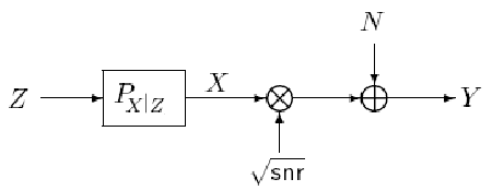
Theorem 1
Consider a system where is chosen from a code and transmitted over a Gaussian channel with signal to noise ratio . Let denote the output of the Gaussian channel. Let represent side information available about . For this system we have
| (12) |
where is the length of the codeword .
Proof:
This system is similar to the general additive noise channel model shown in Fig. 3. We have
| (13) |
Differentiating both sides with respect to and noting that is independent of we have
| (14) |
Given the channel between and is Gaussian. By using the relationship derived by Guo et al [4] we have
| (15) | |||||
Now integrating both sides with respect to we have
| (16) | |||||
∎
Note that in a typical concatenation scheme, is the input to the inner encoder. However, here we use the term inner code to refer to a set of constraints satisfied by . This difference will me made clear in example 2.
Corollary 1
For any code of rate
| (17) |
where represents a length codeword, represents the received signal when is transmitted over an AWGN channel with signal to noise ratio and is the MMSE is estimating given that is the received signal when a codeword was transmitted.
Proof:
Follows from Theorem 1 when there is no side information as . ∎
To plot the transfer characteristic of a component code, it is assumed that the a priori information is from a Gaussian channel. For a true APP decoder, . For the outer code in a concatenation scheme, the in (16), corresponds to the SNR of the a priori channel. Hence, if we plot the MMSE at the output, , as a function of the a priori snr then the area under the curve is equal to the rate of the code times .

Example 1
In Fig. 4 we plot the MMSE as a function of SNR for different rate 1/2 codes. It can be seen that the area under the MMSE curve for the different codes is nearly the same. Numerical computations show that the area is nearly .
In context of iterative decoding, corollary 1 provides a nice relationship between the area under the MMSE vs SNR curve and the rate of an outer code. Theorem 1 links the area under the MMSE vs SNR curve of an inner code to an information theoretic quantity but its relation to the maximum rate supported is not clear. In the following lemma, for a special case, when the outer code is chosen independent of the inner code, we derive a relationship between the maximum outer code rate supported and the area under the MMSE vs a priori snr curve of the inner decoder. Note however, that this special case is what is typically encountered in iterative decoding.

Example 2
Consider the design of a good LDPC code designed for an AWGN channel with signal to noise ratio . We can treat this as a concatenated code where represent the edges and the channel observations. In this case, the inner code represents the restrictions imposed on by the irregular repeat code (Fig. 5). The outer code is a single parity check (SPC) code. We are interested in finding a relationship between the rate of the SPC outer code and the area under the MMSE chart for the inner irregular repeat code. In this case it can be easily seen that the rate of the outer code is bounded above by . The following Lemma generalizes this result.
Lemma 1
If an outer code is chosen independent of the inner code , then, the maximum rate of the outer code that can be used while achieving a vanishing probability of error is given by where represents the channel observation and represents length of . We will refer to this upper bound as .
Proof:
Let be the length of the outer codewords and let represent a length vector. Consider a sequence of length . We say if is a sequence in for all . Similarly we say if is a sequence in for all . We say that and are chosen independently if for a random sequence the events and are independent, i.e., .
The number of length sequences that belong to is . Number of length sequences that belong to is . We have
| (18) |
and the number of sequences that belong to both and is
| (19) |
If with some choice of outer code, the decoder is always able to recover from the channel observations, then the total number of sequences should be less than . Therefore we have
| (20) |
which implies
| (21) |
∎
In the general case (when the outer code is not independent of the inner code), there seems to be no such relationship. For example, consider the LDPC code in Example 2 but consider another outer code constructed from a good rate code () by repeating , the th coded bit, times, where is the degree of the th bit node. In this case the rate of the outer code is . Its relationship to is not straightforward.
The inner decoder has side information about the coded bits from the channel output apart from the a priori information. The transfer characteristics is obtained by increasing the snr of the a priori channel from to . The outer code and inner code are usually separated by a random interleaver which makes the inner code and outer code independent. Therefore from Theorem 1 and Lemma 1 it follows that for an inner decoder, the area under the plot of MMSE at the output against snr of the a priori channel is equal to , where is the maximum rate of outer code supported by the inner code. This can be easily verified for the following examples.
Example 3
Consider an uncoded AWGN channel with signal to noise ratio as an inner code. Let be the transmitted bit and let be the received signal. Let be the output when is sent over another AWGN channel with snr . Clearly, MMSE in estimating from and is same as MMSE in estimating X from the output of an AWGN channel with an snr of . We have
| (22) | |||||
| (23) |
Example 4
Consider an uncoded erasure channel with erasure probability as an inner code. Let equiprobable bits be the transmitted bits and let be the received signal. Let be the output when is sent over an AWGN channel with snr . We have . Therefore
Hence which is exactly the capacity of this channel.
Example 5
Consider an inner code corresponding to an LDPC code over an AWGN channel. Let represent the edges, the a priori messages and let represent the channel information at the bit nodes. The MMSE for an edge connected to a bit node of degree is . Let and represent the degree profile of the LDPC code in edge perspective. We have
For an LDPC code that works well at , we have
It is interesting to compare the area property derived here with that derived by Ashikhmin et al in [2]. It was shown that the area under the EXIT curve, when both the a priori and extrinsic information can be modelled to be from erasure channels, is given by
| (24) |
(24) was obtained by modifying equations (22), (23) in [2] to suit the notation used in this paper.
In the special case when the area becomes . For an outer code of rate the area is therefore is . For some specific inner codes , it was shown that is the maximum rate of the outer code that can be used in iterative decoding to achieve error free communication.
In this paper, we have proved that is indeed the maximum rate of outer code that can be used for reliable communication when the outer code and inner code are independently chosen. This makes the area property derived for EXIT charts more concrete.
We note that in the case when , the simple relationship between the area under the EXIT chart and rate does not hold. However the relationship between area and rate of the outer code and the relationship between area and for the inner code continue to hold for the MMSE vs SNR plot.
IV-A Area Property for MSE chart
Let us assume that the bits about which information is exchanged in an iterative decoding scheme (usually the coded bits of the outer code) are equiprobable. Further, let the a priori and the extrinsic information can be modelled as though the bits were transmitted over an AWGN channel. Let us refer to the SNRs of these channels as and . We first note that if a true APP decoder is employed, MSE is equal to the MMSE. We denote the MMSE corresponding to the a priori, the extrinsic, and the output LLR by , and respectively.
We will refer to a plot of versus as an MSE transfer curve. An MSE chart then has two MSE transfer curves, one for the inner decoder and one for the outer decoder. The area properties proved so far are for a plot of the (not ) versus the . With the Gaussian assumption, the vs plot can be generated from the MSE transfer curve using the transformation . The area properties derived thus apply for the MSE transfer curve under this transformation. For convenience, we use and to denote and , respectively. We will use subscripts and to refer to quantities corresponding to the inner and outer decoders.
Lemma 2
If the a a priori and extrinsic information can be represented as information from Gaussian channels then for a rate code we have
Proof:
Consider the transfer curve as a continuous curve from to by connecting any discontinuity in by vertical lines. With every point on the transfer curve associate a variable . The reason for introducing this variable is to make it easy to handle the possibility discontinuity of the MSE transfer curve. It is easy to see that and are both continuous and increasing functions of such that and are at and at .
∎
Lemma 3
For an inner code when the a a priori and extrinsic information can be represented as information from Gaussian channels then the maximum supported outer code rate () is given by
The proof is similar to the proof in the previous lemma.
Example 6
Consider a repetition code of rate . In this case when the a priori information is from an AWGN channel of snr then the extrinsic information can be modelled as information from a Gaussian channel of snr . We have
| (25) |
This verifies Lemma 2.
V Optimality of Matching
In this section we prove that the MSE curve of the outer code has to be matched to the MSE curve of the inner code when the extrinsic information resembles that from an AWGN channel.
Lemma 4
For two codes and such that , with equality only when the two curves overlap.
Proof:
We have
It is easy to see that equality occurs only when the two curves overlap. ∎
From Corollary 1 and Lemma 3 it follows that a code that is matched exactly to the channel has a rate equal to the rate supported by the inner code. Therefore from Lemma 4 it is easy to see that any outer code whose flipped MSE curve lies below the inner code and is not matched to the inner code has a rate lesser than that supported by the inner code.
We note that under the Gaussian assumption the MSE curve and EXIT curve are related by a one to one function. Therefore since matching is optimal for MSE chart, it is optimal for EXIT charts.
As a consequence of the results derived so far, under the Gaussian assumptions, the following properties hold.
- 1.
With Gaussian assumption on messages from outer decoder to inner decoder.
(26) (27) and for the iterative decoder to converge to the correct codeword . Here and are used to denote the MMSE expressed as a function of the a priori and the extrinsic snr respectively.
- 2.
With Gaussian assumption on messages from inner decoder to outer decoder, we have
(28) (29) and for the iterative decoder to converge to the correct codeword .


Depending on the distribution of the exchanged messages, one of the above mentioned properties may be used to analyze and design component codes. For example, in an LDPC code the bit to check messages closely resembles information from an AWGN channel. In this case we plot MMSE against SNR extrinsic for the inner code and against SNR a priori for the outer code. In Fig. 6 we plot these curves for a rate 0.5 LDPC code that was designed using EXIT charts [6] for an snr of 0.5dB. The degree profile designed LDPC code is , , , and, . The threshold for a bit error rate of is .55dB. The threshold predicted using these curves is 0.51dB. In Fig. 7 we plot these curve for a (3,6) LDPC code. The threshold predicted is 1.05dB and the actual threshold is around 1.1dB.
VI Area Property of Capacity Achieving Codes over AWGN channel
The optimality of matching proved in the previous section assumed that the extrinsic information resembles information from an AWGN channel. In this section we prove the optimality of matching for the AWGN channel without making any assumption on the extrinsic information. We show that the EXIT curve of any capacity achieving code is flat and is matched to the channel. It is also seen that the area under the EXIT curve of any rate capacity achieving code is equal to .
Consider a capacity achieving binary code of rate being transmitted over an AWGN channel with signal to noise ratio . Since the code decodes perfectly when the MMSE in estimating the transmitted codeword from the received symbols is 0. Therefore from Corollary 1 we get
| (30) | |||||
| (31) | |||||
| (32) |
The inequality in (30) is because MMSE error in estimating from both and is always less that MMSE error in estimating from . It is also easy to prove that only when . (31) follows from (11).
Since the inequalities in (30) and (31) have to be equalities. Therefore we have . We also have
| (33) |
Since , from (33) it follows that for almost every .
Now, using the fact that MMSE in both the cases is a decreasing function of and the fact that is continuous, it can be shown that
| (34) |
It is easy to see that the MMSE estimate . Therefore for we have
| (35) |
Therefore when .
When , when is transmitted. Since we have when . Similarly we have when . Therefore when .
VII Conclusion
We proposed a new measure based on MSE for analyzing the convergence behavior of iterative decoding schemes. This measure is robust and can be computed without the knowledge of the transmitted bits. Under Gaussian assumptions, we showed a mapping from the MSE chart such that for any code the area under the map is equal to the rate. We used this to prove that curve fitting is optimum in the MSE chart and then extended it to the EXIT chart case. For the AWGN channel, without making any assumptions on the distribution of extrinsic LLRs, we showed that capacity achieving codes have an EXIT chart that is flat and matched to the channel .
References
- [1] M. Tuchler, S. ten Brink, and J. Hagenauer, “Measures for tracing convergence of iterative decoding algorithms,”Proc. 4th Int. ITG Conf. on Source and Channel Coding, Berlin, Germany, Jan.2002.
- [2] A. Ashikhmin, G. Kramer, and S. ten Brink, “Extrinsic Information Transfer Functions: Model and Erasure Channel Properties,”IEEE Trans. on Inform. Theory to appear 2004.
- [3] K. Narayanan, “Effect of precoding on the convergence of turbo equalization for partial response channels,” IEEE Journal on Sel. Areas in Comm., vol. 19, pp. 686-698, April 2001.
- [4] D. Guo, S. Shamai and S. Verdu, “Mutual information and MMSE in Gaussian channels,” Proceedings 2004 IEEE International Symposium on Information Theory, Chicago, IL, USA, June 2004.
- [5] S. ten Brink, “Convergence behaviour of iteratively decoded parallel concatenated codes,” IEEE Trans. on Commun., vol. 49, pp. 1727-1737, Oct 2001.
- [6] S. ten Brink, G. Kramer, and A. Ashikhmin, “Design of low-density parity-check codes for modulation and detection,”IEEE Trans. on Commun., vol. 52, pp. 670-678, April 2004.
- [7] K. Bhattad and K.R. Narayanan, ”An MSE based transfer chart to analyze iterative decoding schemes,” 42nd Allerton Conference on Communications, Control and Computing, Monticello, IL, Oct 2004.
- [8] M. Peleg, A. Sanderovich and S. Shamai (Shitz), ”On Extrinsic Information of Good Codes Operating Over Discrete Memoryless Channels,”available for download from http://arxiv.org/ftp/cs/papers/0504/0504028.pdf