Sparse Covariance Selection via
Robust Maximum Likelihood Estimation

For a given covariance matrix $\Sigma\in{\mbox{\bf S}}_{+}^{n}$, and reals numbers $0\leq\alpha<\beta$, our problem is formulated as

with variable $X\in{\mbox{\bf S}}^{n}$, and $\|X\|_{1}:=\sum_{i,j=1}^{n}|X_{ij}|$. The parameter $\rho>0$ controls the size of the penalty, hence the sparsity of the solution. Here $\langle\Sigma,X\rangle=\mathop{\bf Tr}\Sigma X$ denotes the scalar product between the two symmetric matrices $\Sigma,X$. The penalty term involving the sum of absolute values of the entries of $X$ is a proxy for the number of its non-zero elements, and is often used in regression techniques, such as LASSO in [Tib96], when sparsity of the solution is a concern. In our model, the bounds $(\alpha,\beta)$ on the eigenvalues of $X$ are fixed, and user-chosen; although we allow $\alpha=0$, $\beta=+\infty$ in our model, such bounds are useful in practice to control the condition number of the solution.

For $\rho=0$, and provided $\Sigma\succ 0$, problem (1) has a unique solution $X^{\ast}=\Sigma^{-1}$, and the corresponding maximum-likelihood estimate $\hat{\Sigma}=\Sigma$. Due to noise in the data, in practice, the sample estimate $\Sigma$ may not have a sparse inverse, even if the underlying graphical model exhibits conditional independence properties; by striking a trade-off between maximality of the likelihood and number of non-zero elements in the inverse covariance matrix, our approach is potentially useful at discovering structure, precisely conditional independence properties in the data. At the same time, it serves as a regularization technique: when $\Sigma$ is rank-deficient, there is no well-defined maximum-likelihood estimate, whereas it can be shown that the solution to problem (1) is always unique and well-defined for $\rho>0$, even if $\alpha=0$ and/or $\beta=\infty$.

In the case when $\alpha=0$, $\beta=\infty$, we write (1) as

where $\|U\|_{\infty}$ denotes the maximal absolute value of the entries of $U$. This corresponds to seeking an estimate with maximal worst-case likelihood, over all componentwise bounded additive perturbations $\Sigma+U$ of the sample covariance matrix $\Sigma$. Such a ”robust optimization” interpretation can be given to a number of estimation problems, most notably support vector machines for classification.

The above leads to the following equivalent, dual problem (with $\alpha=0$, $\beta=\infty$):

Note that the diagonal elements of an optimal $U$ are simply $U_{ii}=\rho$. The corresponding covariance matrix estimate is $\hat{\Sigma}:=\Sigma+U$. Since the above dual problem has a compact feasible set, both primal and dual problems are equivalent.

In the case when $\alpha=0$, $\beta=\infty$, we can derive finite, a priori bounds on the condition number of the solution. Indeed, we can show that we can always assume $\alpha(n)\mathbf{\mathbf{I}}_{n}\preceq X\preceq\beta(n)\mathbf{\mathbf{I}}_{n}$, where $\alpha(n):=1/(\|\Sigma\|+n\rho)$ and $\beta(n)=n/\rho$. These bounds guarantee strict convexity of the objective, as well as existence, boundedness and uniqueness of the solution when $\rho>0$, even if no bounds are set a priori.

Of course, problem (1) is convex and can readily be solved using interior point methods (see [BV04] for example). However, such second-order methods become quickly impractical for solving (1), since the corresponding complexity to compute an $\epsilon$-suboptimal solution is $O(n^{6}\log(1/\epsilon))$. The authors of [DRV05] developed interior-point algorithms to solve a problem related to (1), where a (sparse) structure of the solution is known a priori. Here our focus is on relatively large, dense problems, for which a solution of moderate accuracy is enough. Note that we cannot expect to do better than $O(n^{3})$, which is the cost of solving the non-penalized problem for dense covariance matrices $\Sigma$. The recently-developed first-order algorithms due to [Nes03] trade-off a better dependence on problem size against a worse dependence on accuracy, usually $1/\epsilon$ instead of its logarithm. The method we describe next has a complexity of $O(n^{4.5}/\epsilon)$. This is a substantial improvement over interior-point methods when $\epsilon$ is not too small, which is often the case in practice. In addition, the memory space requirement of the first-order method is much lower than that of interior-point methods, which involve storing a dense Hessian, and hence become quickly prohibitive with a problem having $O(n^{2})$ variables.

We can write (2) in the format given in [Nes03]:

where we define $\hat{f}(X)=-\log\det X+\langle\Sigma,X\rangle$, $A=\rho I_{n^{2}}$, and ${\cal Q}_{1}:=\left\{X\in{\cal S}^{n}~:~\alpha\mathbf{\mathbf{I}}_{n}\preceq X\preceq\beta\mathbf{\mathbf{I}}_{n}\right\}$, ${\cal Q}_{2}:=\left\{U\in{\cal S}^{n}~:~\|U\|_{\infty}\leq 1\right\}$.

To ${\cal Q}_{1}$ and ${\cal Q}_{2}$ we now associate norms and so-called prox-functions. For ${\cal Q}_{1}$, we use the Frobenius norm, and a prox-function

The function $d_{1}$ is strongly convex on ${\cal Q}_{1}$, with a convexity parameter of $\sigma_{1}=1/\beta^{2}$, in the sense that $\nabla^{2}d_{1}(X)[H,H]=\mathop{\bf Tr}(X^{-1}HX^{-1}H)\geq\beta^{-2}\|H\|_{F}^{2}$ for every $H$. Furthermore, the center of the set, $X_{0}:=\arg\min_{X\in{\cal Q}_{1}}\>d_{1}(X)$ is $X_{0}=\beta\mathbf{\mathbf{I}}_{n}$, and satisfies $d_{1}(X_{0})=0$. With our choice, we have $D_{1}:=\max_{X\in{\cal Q}_{1}}\>d_{1}(X)=n\log(\beta/\alpha)$.

To ${\cal Q}_{2}$, we also associate the Frobenius norm, and the prox-function $d_{2}(U)=\|U\|_{F}^{2}/2$. With this choice, the center $U_{0}$ of ${\cal Q}_{2}$ is $U_{0}=0$. Furthermore, the function $d_{2}$ is strictly convex on its domain, with convexity parameter with respect to the $1$-norm $\sigma_{1}=1$, and we have $D_{2}:=\max_{U\in{\cal Q}_{2}}\>d_{2}(U)=n^{2}/2$.

The function $\hat{f}$ has a gradient that is Lipschitz-continuous with respect to the Frobenius norm on the set ${\cal Q}_{1}$, with Lipschitz constant $M=1/\alpha^{2}$. Finally, the norm (induced by the Frobenius norm) of the operator $A$ is $\|A\|=\rho$.

The method is based on replacing the objective of the original problem, $f(X)$, with $f_{\epsilon}(X)$, where $\epsilon>0$ is the given desired accuracy, and $f_{\epsilon}$ is the penalized function involving the prox-function $d_{2}$:

The above function turns out to be a smooth uniform approximation to $f$ everywhere, with maximal error $\epsilon/2$. Furthermore, the function $f_{\epsilon}$ is Lipschitz-continuous, with Lipschitz constant given by $L(\epsilon):=M+D_{2}\|A\|^{2}/(2\sigma_{2}\epsilon)$. A specific gradient algorithm for smooth, constrained convex minimization is then applied to the smooth convex function $f_{\epsilon}$, with convergence rate in $O(\sqrt{L(\epsilon)/\epsilon})$. Specifically, the algorithm is guaranteed to produce an $\epsilon$-suboptimal solution after a number of steps not exceeding

Choose $\epsilon>0$ and set $X_{0}=\beta\mathbf{\mathbf{I}}_{n}$, and proceed as follows.

For step $1$, the gradient of $f_{\epsilon}$ is readily computed in closed form, via the computation of the inverse of $X$. Step $2$ essentially amounts to projecting on ${\cal Q}_{1}$, and requires an eigenvalue problem to be solved; likewise for step $3$. In fact, each iteration costs $O(n^{3})$. The number of iterations necessary to achieve an objective with absolute accuracy less than $\epsilon$ is given in (4) by $N(\epsilon)=O(n/\epsilon)$ (if $\rho>0$). Thus, the overall complexity when $\rho>0$ is $O(n^{4.5}/\epsilon)$, as claimed.

In our experiments, we have used a preliminary version of Nesterov’s method with $\alpha=0$ and $\beta=\infty$ that, instead of working on the primal (1), addresses the dual (2). The algorithm is essentially the same as that presented in section 3, with the following setup. Define ${\cal Q}_{1}:=\{x~:~U\in{\cal S}^{n}~:~\|U\|_{\infty}\leq 1\}$, ${\cal Q}_{2}=\{U\in{\cal S}_{+}^{n}~:~\mathop{\bf Tr}U\leq n/\rho\}$, and

To simplify the projections required by the algorithm, we make the assumption that $\rho$ is small enough to ensure that ${\cal Q}_{1}$ is entirely included in the cone of positive semidefinite matrices. In practice, we have found that the algorithm does well, even when this condition does not hold. As in section 3, each step of this algorithm costs $O(n^{3})$ operations.

To ${\cal Q}_{1}$, we associate the Frobenius norm in ${\mbox{\bf R}}^{n\times n}$, and a prox-function defined for $x\in{\cal Q}_{1}$ by $d_{1}(X)=(1/2)\|X\|_{F}^{2}$; the center of ${\cal Q}_{1}$ with respect to $d_{1}$ is $X_{0}=0$, and $D_{1}=\max_{X\in{\cal Q}_{1}}\>d_{1}(X)=\rho^{2}n^{2}/2$. Furthermore, the function $d_{1}$ is strictly convex on its domain, with convexity parameter with respect to the Frobenius norm $\sigma_{1}=1$. For ${\cal Q}_{2}$ we use the dual of the standard matrix norm (denoted $\|\cdot\|^{\ast}_{2}$), and a prox-function $d_{2}(U)=\mathop{\bf Tr}(U\log U)+\log n$, where $\log$ refers to the matrix (and not componentwise) logarithm. The center of the set ${\cal Q}_{2}$ is $U_{0}=n^{-1}\mathbf{\mathbf{I}}_{n}$, and $d_{2}(U_{0})=0$. We have $\max_{u\in{\cal Q}_{2}}\>d_{2}(u)\leq\log n:=D_{2}$. The convexity parameter of $d_{2}$ on its domain with respect to $\|\cdot\|_{2}^{\ast}$, is bounded below by $\sigma_{2}=1/2$ [BTN04]. Finally, the norm of the operator $A$, with respect to the Frobenius norm and the dual of the standard norm, is $1$.

We now describe an algorithm based on block-coordinate descent, which solves the dual problem (2) by optimizing over one column/row pair at a time. For simplicity, we consider the case when $\alpha=0$ and $\beta=\infty$, which corresponds to providing no a priori bounds on the condition number of the solution.

The algorithm is initialized with the estimate $\hat{\Sigma}=\Sigma+\rho I\succ 0$, since the optimal diagonal values of $U$ in (2) are simply $\rho$. To update $\hat{\Sigma}$, we solve (2) where all elements in $U$, except the off-diagonal values of one column (and corresponding row), are fixed. Using a permutation of rows and columns, we can always express the problem as one of optimizing over the last column/row pair:

where inequalities are understood componentwise, and the current estimate $\hat{\Sigma}$ of the covariance matrix is partitioned into four blocks, with $\hat{\Sigma}_{11}$ the upper-left $(n-1)\times(n-1)$ block, and $(\hat{\Sigma}_{12},\hat{\sigma}_{22})$ the last column. The sub-problem (5) reduces to a simple box-constrained quadratic program. Specifically, the corresponding column/row $\hat{\Sigma}_{12}$ of the current estimate $\hat{\Sigma}$ is updated with $\hat{\Sigma}_{12}+u^{\ast}$, where

The stopping criterion we can use involves checking if the primal-dual gap of the problem (2) is less than a given tolerance $\epsilon$, which translates as $\langle\Sigma,X\rangle+\rho\|X\|_{1}\leq n+\epsilon$, where $X=\hat{C}^{-1}$. In practice though, we have found that a fixed number of sweeps (say, $K=4$) through all column/row pairs is usually enough.

It can be proven that the algorithm converges, however we do not know the complexity of the algorithm. A simple modification of it, where we impose a condition number constraint on the estimate $\hat{\Sigma}$ at each column/row update, can be shown to converge in $O(n^{6})$. Hence, the dual BCD algorithm is not really competitive from the theoretical complexity point of view, but the version given here remains attractive because it is simple to implement, and does well in practice. Since each column/row update costs $O(n^{3})$, when only a few, fixed number $K$ of sweeps through all columns is done, the cost is $O(Kn^{4})$.

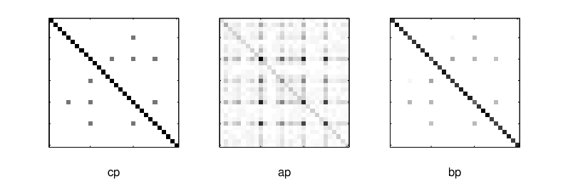
To illustrate our method we consider a synthetic example constructed by adding noise to a covariance matrix which has a sparse inverse. Precisely, we take a random $n\times n$ sparse matrix $A$, with $n=30$, and then add a uniform noise of magnitude $\sigma=.13$ to its inverse to form our matrix $\Sigma$. Our concern here is to check if our methods reach a degree of precision sufficient to recover the problem structure, despite the noise masking it. Figure 1 shows the original sparse matrix $A$, the noisy inverse $\Sigma^{-1}$ and the solution $X$ of problem (1) solved using Nesterov’s algorithm detailed in section 4 with parameter $\rho=\sigma$.

Of course, the simple example above assumes that we set $\rho$ equal to the noise level $\sigma$, so we look at what happens when the value of $\rho$ is set above or below $\sigma$. In Figure 2 on the left, we solve problem (1) for various values of $\rho$. We plot the minimum $\min\{X_{ij}:A_{ij}\neq 0\}$ (solid) and mean (dash-dot) magnitude of those coefficients in the solution $X$ corresponding to non zero coefficients in $A$ (solid line) against the maximum $\max\{X_{ij}:A_{ij}=0\}$ (dashed line) and mean (dotted line) magnitude of coefficients in $X$ corresponding to zeros in $A$ (we only consider off-diagonal coefficients). For all values of $\rho$ within the interval $V$ shown in Figure 2, the minimum is larger than the maximum, meaning that for all thresholding levels between the minimum and maximum, we exactly recover the original matrix $A$. As we can observe, the range $V$ of values of $\rho$ for which this happens is fairly large and so is the gap between the minimum and maximum within the interval $V$.

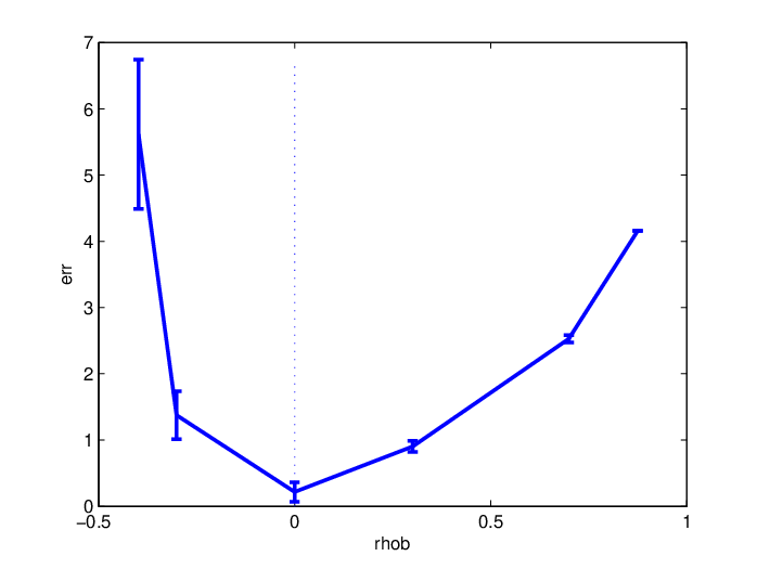
In Figure 2 on the right, for various values of $\rho$, we randomly sample 10 noisy matrices $\Sigma$ with $n=50$ and $\sigma=.1$ and compute the number of misclassified zeros and nonzero elements in the solution to (1) produced by the block coordinate descent method. We plot the average percentage of errors (number of elements incorrectly set to zero plus number of elements incorrectly kept nonzero, divided by $n^{2}$), as well as error bars corresponding to one standard deviation.

We now compare Nesterov’s and coordinate descent algorithms on a set of randomly generated examples. The noisy matrix $\Sigma$ is generated as above and we plot in Figure 3 CPU time against problem size for various $n$ and duality gap versus CPU time in seconds for a random problem of size $100$ with a few nonzero coefficients. In practice, a low-precision solution to (1) is sufficient to identify most of the nonzero coefficients in the original matrix $A$. In Figure 4 we show the classification error made by the solution on the example with $n=100$. Typical computing time for a problem with $n=300$ is about 20 minutes. (All CPU times computed on a 1.5Ghz PowerBook G4 laptop).

The authors would like to thank Francis Bach, Peter Bartlett and Martin Wainwright for enlightening discussions on the topic.

References

- [Bil99] J. A. Bilmes. Natural statistic models for automatic speech recognition. Ph.D. thesis, UC Berkeley, Dept. of EECS, CS Division, 1999.
- [Bil00] J. A. Bilmes. Factored sparse inverse covariance matrices. IEEE International Conference on Acoustics, Speech, and Signal Processing, 2000.
- [BTN04] A. Ben-Tal and A. Nemirovskii. Non-euclidean restricted memory level method for large-scale convex optimization. MINERVA Working paper, 2004.
- [BV04] S. Boyd and L. Vandenberghe. Convex Optimization. Cambridge University Press, 2004.
- [CG99] S. S. Chen and R. A. Gopinath. Model selection in acoustic modeling. EUROSPEECH, 1999.
- [Dem72] A. P. Dempster. Covariance selection. Biometrics, 28(1):157–75, 1972.
- [DHJ+04] A. Dobra, C. Hans, B. Jones, J.R. J. R. Nevins, G. Yao, and M. West. Sparse graphical models for exploring gene expression data. Journal of Multivariate Analysis, 90(1):196–212, 2004.
- [DRV05] J. Dahl, V. Roychowdhury, and L. Vandenberghe. Maximum likelihood estimation of gaussian graphical models: numerical implementation and topology selection. UCLA preprint, 2005.
- [DW04] A. Dobra and M. West. Bayesian covariance selection. Working paper, ISDS, Duke University, 2004.
- [HLP05] J. Z. Huang, N. Liu, and M. Pourahmadi. Covariance selection and estimattion via penalized normal likelihood. Wharton Preprint, 2005.
- [JCD+04] B. Jones, C. Carvalho, C. Dobra, A. Hans, C. Carter, and M. West. Experiments in stochastic computation for high-dimensional graphical models. ISDS Discussion Paper 04-01, 2004.
- [Nes03] Y. Nesterov. Smooth minimization of nonsmooth functions. CORE discussion paper 2003/12 (Accepted by Math. Prog.), 2003.
- [Tib96] R. Tibshirani. Regression shrinkage and selection via the lasso. Journal of the Royal statistical society, series B, 58(267-288), 1996.