-Cycle Double Covers of Cubic GraphsThanks: Corresponding author (valmir@cos.ufrj.br).
Abstract
A cycle double cover (CDC) of an undirected graph is a collection of the graph’s cycles such that every edge of the graph belongs to exactly two cycles. We describe a constructive method for generating all the cubic graphs that have a -CDC (a CDC in which every cycle has length ). As an application of the method, we prove that all such graphs have a Hamiltonian cycle. A sense of direction is an edge labeling on graphs that follows a globally consistent scheme and is known to considerably reduce the complexity of several distributed problems. In [9], a particular instance of sense of direction, called a chordal sense of direction (CSD), is studied and the class of -regular graphs that admit a CSD with exactly labels (a minimal CSD) is analyzed. We now show that nearly all the cubic graphs in this class have a -CDC, the only exception being .
Keywords: Cycle double covers, Cubic graphs, Chordal sense of direction, Circulant graphs, Hexagonal tilings, Fullerenes, Polyhexes.
1 Introduction
In this paper we consider connected undirected graphs having no multiple edges or self-loops. For terminology or notation not defined here we refer the reader to [3]. A cycle double cover (CDC) of a graph is a collection of cycles in such that every edge of belongs to exactly two of the cycles. It can be easily seen that a necessary condition for a graph to have a CDC is that the graph be -edge-connected. It has been conjectured that this condition is also sufficient [13, 12], but the conjecture has remained unsettled and constitutes one of the classic unsolved problems in graph theory.
A -cycle double cover (-CDC), for , is a CDC whose every cycle has length . Previous results on -CDC’s are the ones in [1, 14, 15], all motivated by the relationship between -CDC’s and embeddings on surfaces. In [1], the -regular graphs that have a -CDC are studied and some results are shown to carry over, by duality, to the class of girth- cubic graphs that have a -CDC. This latter class is characterized in [14], and in [15] deciding whether a graph has a -CDC is proven NP-complete.
In this paper we introduce a constructive method for generating all the cubic graphs that have a -CDC, and prove in addition that all such graphs are Hamiltonian. For the particular case of girth- cubic graphs, these contributions provide both an alternative to the method of [14] and an answer to the question raised in [1] regarding the graphs’ Hamiltonicity. Graphs in this case can also be viewed as hexagonal tilings of the torus (the orientable surface of genus ) or of the Klein bottle (the non-orientable surface of cross-cap number ; cf. [14]) and have many applications in chemistry, where they are also called toroidal and Klein-bottle fullerenes [4] or polyhexes [8].
Our initial motivation, though, has been the relationship between -CDC’s and the chordal sense of direction (CSD) [7] of a graph. A sense of direction is an edge labeling on graphs that follows a globally consistent scheme and is known to considerably reduce the complexity of several distributed problems [5].
In the particular case of a CSD, to be defined precisely in Section 6, we have in another study characterized the -regular graphs that admit a CSD with exactly labels [9], also called a minimal CSD (MCSD). A further contribution of the present study is to demonstrate that, except for , every cubic graph that has an MCSD also has a -CDC. Since in [9] we also prove that the class of regular graphs that have an MCSD is equivalent to that of circulant graphs, this contribution also holds for cubic circulant graphs. We note that circulant graphs have great practical relevance due to their connectivity properties (small diameter, high symmetry, etc.), which render them excellent topologies for network interconnection, VLSI, and distributed systems [2].
The following is how we organize the remainder of the paper. We start in Section 2 with preliminary results on -CDC’s and their cycles. Then we move in Section 3 to the introduction of our method to generate all cubic graphs that have a -CDC. In Section 4 we describe the method’s details by explaining how it is applied for each possible girth value. Our method never generates duplicates or misses a graph, as we explain in Section 5 along with a demonstration that all cubic graphs that have a -CDC are Hamiltonian. The relationship to MCSD’s is discussed in Section 6, and then we close in Section 7 with concluding remarks.
2 Preliminaries
We henceforth assume that is a cubic graph on vertices and edges and that it has a -CDC. Clearly, and is necessarily even. We say that a cycle of such a -CDC covers a certain edge whenever that edge belongs to . Let us initially establish some properties of the cycles of a -CDC of .
Lemma 1.
Every -CDC of has cycles.
Proof.
Let be the number of cycles in a -CDC of . As each edge belongs to two of the cycles, we have . And because , it follows that , thence . ∎
Lemma 2.
No two cycles of a -CDC of share a path containing more than one edge.
Proof.
Suppose, contrary to our aim, that is a path of length in belonging to two cycles, say and , of the -CDC. Let be the other vertex adjacent to . The two cycles of the -CDC that cover the edge must also cover either or . However, both and are already covered by and , a contradiction. ∎
Lemma 3.
Every vertex of belongs to exactly three cycles of a -CDC of .
Proof.
By Lemma 2, each of the cycles going through a vertex must cover a distinct pair of edges incident to . The result follows from recognizing that there exist such pairs. ∎
Now, for and any two cycles of a -CDC of , let be the number of edges covered by both and , and the number of cycles of the -CDC, excluding , that have at least one edge in common with . We can bound these numbers as follows.
Lemma 4.
If and are cycles in a -CDC of , then .
Proof.
The lower bound is trivial and corresponds to and being edge-disjoint. As for the upper bound, it follows directly from Lemma 2, since requires and to share a path containing more than one edge. ∎
Lemma 5.
If is a cycle in a -CDC of , then .
Proof.
The lower bound follows from Lemma 2 and corresponds to having all three edges in each of its two possible sets of noncontiguous edges in common with a same cycle of the -CDC. The upper bound is trivial and corresponds to the case in which shares each of its edges with a different cycle of the -CDC. ∎
We can also characterize the graphs that effectively attain the upper bound of Lemma 4. As we see in Lemma 6 below, each such graph has a three-cycle -CDC whose cycles all attain the lower bound of Lemma 5 as well. We first review some definitions. A chord is an edge interconnecting two noncontiguous vertices of a cycle. Let be a cycle of even length. A Möbius ladder on vertices, denoted by , is the graph obtained by adding chords between all vertex pairs that are edges apart on ( is shown in Figure 1(a)). For a divisor of , an -layer torus on vertices, denoted by , is an mesh in which maximally distant vertices on the same row or column are connected to each other ( is shown in Figure 1(b)).
 |
 |
|---|---|
| (a) | (b) |
Lemma 6.
If and are cycles in a -CDC of such that , then is isomorphic to either or .
Proof.
In the remainder of the paper, for any graph we use to denote its vertex set and its edge set. Furthermore, we call a cycle fragment any subgraph of a -CDC’s cycle, and a cycle configuration any collection of cycles or cycle fragments of a -CDC.
3 A recursive method
Having established some restrictions on the cycles that form a -CDC, we are now in position to describe a constructive method for generating cubic graphs that have a -CDC. Let be a proper subgraph of whose vertices have degree or . When we consider the intersection of the cycles of a -CDC of with , we obtain a cycle configuration in such as the one illustrated in Figure 2, where an edge is labeled to indicate that it belongs to the cycles and of the -CDC.
 |
 |
|---|---|
| (a) | (b) |
We say that a vertex is deficient in a certain graph if its degree is less than in that graph. The deficiency of graph is given by , where is the degree of in . Note that the deficient vertices in are exactly the ones that are also deficient in , where for we use to denote the graph obtained from by removing the edges in and the vertices that become isolated after the edge removal. For and as in Figure 2, is the external triangle in part (a) of the figure.
Now suppose that there exists another graph that can replace in in such a way that the resulting graph, call it , is cubic and has a -CDC with the same cycle configuration on the edges of as on the edges of . In other words, suppose that leads to a cubic such that the cycle configuration in remains unchanged from the -CDC of to that of . If such is the case, then must have the same deficiency as (so the resulting is cubic) and also a cycle configuration that completes the one in as needed to yield the -CDC of . For and as in Figure 2, and are as illustrated in Figures 3(a) and 3(b), respectively.
 |
 |
|---|---|
| (a) | (b) |
For the latter condition to be satisfied, the following two properties must hold. First, if are the deficient vertices of (all of degree , by definition), then there has to exist a partition of the deficient vertices of such that and have the same deficiency,11 1 We extend the definition of a graph’s deficiency to that of a vertex or vertex set in the obvious way. . Clearly, necessarily, so has either one degree- vertex or two degree- vertices. By Lemma 3, each degree- vertex in or , or degree- vertex in , has exactly two cycles of the -CDC of going through it along edges of both and , or of and , as the case may be. For and , , let and be the two cycles in , and the two cycles in . The second property is that the fragment of in and the fragment of in both have the same length, and similarly for and .
In the case of Figures 2 and 3, no degree- vertices exist in and the above holds with and , for example. The fragments of and in are and , respectively, while in they are and .
We say that cycle configurations such as the ones of and are equivalent to each other. When it is the case, in addition, that has at least one subgraph that is isomorphic to and all such subgraphs have cycle configurations that are equivalent to that of (hence to that of also), then we say that is self-similar with respect to . This is certainly the case of the and of Figures 2(b) and 3(a), since the triangle of Figure 3(a), when augmented by vertices , , and and the edges that lead to them from the triangle, is isomorphic to the graph in Figure 2(b) with equivalent cycle configuration.
Self-similarity is a property of positive-deficiency graphs and constitutes the core of our method. Before proceeding to a description of the method, we let denote the girth of . In our present case of graphs that have a -CDC, necessarily, and we use the value of to divide our approach into cases, as presented in Section 4.
For a fixed value of in , let be the deficiency- graph on vertices that comprises a length- cycle and additional vertices, each of them connected to a distinct vertex of the cycle. For , is the of Figure 2(b). In general, it is easy to see that every girth- cubic graph having a -CDC has a subgraph isomorphic to with a cycle configuration that is consistent with the -CDC, even though the off-cycle vertices of this subgraph are not always all distinct.22 2 In fact, vertex distinctness holds for all but one single case, specifically one of the cycle configurations of , as we discuss in Section 4.2. For a fixed cycle configuration of , let also be a minimal girth- proper supergraph of which, along with a cycle configuration of its own, is self-similar with respect to .33 3 Notwithstanding the formal generality of this definition, what happens is that, as we show in Sections 4.1 through 4.4, for every valid cycle configuration of there exists only one instance. In the example, is the of Figure 3(a).
Now, a very important observation is that, for , it may be impossible for to exist as defined. The reason is that the cycle configuration of does not necessarily include a complete cycle of the -CDC, while it may happen that every girth- proper supergraph of whose cycle configuration is equivalent to that of , is also a supergraph of an isomorph of whose cycle configuration does include a complete -CDC cycle. We then see that the definition of self-similarity must be modified in the girth- case when the cycle configuration of does not contain a complete -CDC cycle. The modification is that not all subgraphs of that are isomorphic to are required to have cycle configurations equivalent to that of , but rather only those whose cycle configurations do not contain a complete -CDC cycle. That the girth- case should require such an exceptional treatment is not really a surprise, since we are throughout dealing with graphs that have a -CDC, and thence it is only natural that -cycles that are in the -CDC be distinguished from those that are not.
Given the notion of self-similarity, the definitions of and imply that can substitute indefinitely for any isomorph of that has a cycle configuration equivalent to that of , thus generating an infinite sequence of deficiency-, girth- graphs whose first graph is itself. For , such an isomorph is any of the -isomorphs that the current graph has as subgraphs; for , isomorphs whose cycle configuration includes a complete -CDC cycle are excluded if the cycle configuration of does not itself contain a complete -CDC cycle. Turning the resulting graphs into girth- cubic graphs that have a -CDC requires that we define yet another graph based on . This graph is denoted by and its definition, too, depends on what happens in the case.
is in all cases defined to be a girth- supergraph of that has a -CDC. If either or else but the cycle configuration of does not include a complete -CDC cycle, then is furthermore of one of two types:
- (i)
is not a supergraph of .
- (ii)
is a supergraph of such that substituting for causes the girth of to be reduced.
The remaining case is that of when the cycle configuration of does include a complete cycle of the -CDC. In this case, has the following property, in addition to being a girth- supergraph of that has a -CDC:
- (iii)
is a supergraph of and all its -cycles are cycles of the -CDC. In addition, it is such that substituting for causes the appearance of -cycles that are not in the -CDC.
In any of cases (i)–(iii), the -CDC of is assumed to coincide with the cycle configuration of or , depending respectively on whether is a supergraph of only or of as well. It is also curious to note that, if is of type (iii), then in it automatically holds that every -cycle is a cycle of the -CDC; but this already follows from the very definition of , since in this case itself contains a complete -CDC cycle in its cycle configuration.
The reason for making a distinction between these three types is immaterial at this point and will only become clear in Section 4.4, in which we handle the girth- case, and in Section 5 when we argue for the completeness of our method. For the girth- example we have been using as illustration, notice that the of Figure 2(a) is a type-(i) instance of .
One crucial property emerging from the definitions of , , and is that, except for type-(i) instances of , every girth- cubic graph that has a -CDC also has a subgraph isomorphic to with a cycle configuration that renders it self-similar with respect to . So not only is the indefinite substitutability of for true, but it can be used to generate all girth- cubic graphs that have a -CDC, as follows. For each possible cycle configuration of , we identify and all pertinent instances. By starting at each such instance and substituting for indefinitely, ever larger girth- cubic graphs are generated having a -CDC.
4 Applying the method
For each pertinent girth value , in this section we start with and identify all its possible cycle configurations. For each of these cycle configurations, we then expand (along with its cycle configuration, by adding vertices and edges) without disrupting the -CDC nature of its cycle configuration or altering the girth. We do this until and all instances of are obtained.
While expanding we first attempt to generate type-(i) instances of , that is, those that are not supergraphs of . Then we proceed to generating itself and from there we move to expanding towards obtaining the instances of that are supergraphs of , that is, type-(ii) or (iii) instances. It is important to realize that, since and have cycle configurations that are equivalent, carrying the expansion beyond need not attempt the same expansion steps that generated type-(i) instances: doing this would only lead to graphs that already belong to the sequence of graphs generated by substituting for recursively from a type-(i) instance onward. What must be attempted, rather, are expansion steps that failed previously but may now succeed (like those that somehow disrupt the girth or the -CDC when attempted on ).
4.1 The girth- case
We start with the graph of Figure 2(b) as (that is, the core cycle of is ). It is easy to see that the cycle configuration given in Figure 2(b) is the only one that does not violate the restrictions discussed in Section 2. Furthermore, note that the vertices , , and must all remain distinct as we expand , otherwise either the resulting graph would be isomorphic to (which is too small to have a -CDC) or the resulting cycle configuration would be inconsistent with the requirements of a -CDC.
Given the unique cycle configuration for in Figure 2(b), we proceed with the expansion. This is done by completing the cycles , , and . We have two ways of completing : either using an existing vertex () or including a new one. While the former option leads unavoidably to and its cycle configuration shown in Figure 2(a) when applied to all three cycles, the latter results, after a suitable renaming of vertices and cycles, and also unavoidably, in the of Figure 3(a) and its cycle configuration. As noted in Section 3, is of type (i); also, for the reasons given above in the introduction to Section 4, seeking type-(ii) instances of any further is in this case meaningless.
Notice that we can now replace by in , thus obtaining a larger cubic graph of girth (the one in Figure 3(b)) that has a -CDC. This substitution process can proceed recursively, always generating cubic graphs of girth with a -CDC. The graphs resulting from the second and third iterations are shown in Figure 4.
 |
 |
|---|---|
| (a) | (b) |
4.2 The girth- case
We start by analyzing all the possible cycle configurations of . In Figures 5(a)–(c), the cycle configurations of that infringe neither Lemma 2 nor Lemma 3, and also do not lead to the existence of a cycle with length smaller than in the -CDC, are presented. Note that vertices , , , and are all distinct in these graphs. The cases in which these vertices may coincide will be treated later.
 |
 |
 |
| (a) | (b) | (c) |
For each cycle configuration shown in Figure 5, we must identify and . We denote by the graph with the cycle configuration of Figure 5(a), and likewise and refer to the expansions of . We proceed similarly in the cases of Figures 5(b) and 5(c).44 4 The expansion of into a instance has two possible outcomes, which we denote by and .
The only possibilities for are the , , and of Figure 6. As for , the only possibilities that Lemmas 2 and 3 allow are the , , , and of Figure 7. Notice that each of , , and is isomorphic to , and that is isomorphic to . Also, they are all type-(i) instances of .
 |
 |
|---|---|
| (a) | (b) |
 |
| (c) |
 |
 |
|---|---|
| (a) | (b) |
 |
 |
|---|---|
| (c) | (d) |
It is illustrative to notice also that the cycle configurations of and are in fact equivalent to each other, and also that every subgraph of that is isomorphic to has a cycle configuration that is equivalent to that of . That is, is indeed self-similar with respect to and does as such allow for recursive substitutions of for starting at . Except for the initial , since it is of type (i), all -isomorphic subgraphs of the resulting graphs have cycle configurations equivalent to that of .55 5 In Section 5, we use this property to argue for the uniqueness of each graph generated in the process. The cases of and with (or ) and of and with are entirely analogous.
Now let us consider the cases in which vertices , , , and are not necessarily distinct. It is easy to see that the only way for this to happen without altering the girth is to let or . If either or , then clearly the cycle configurations of Figures 5(a) and 5(c) acquire a cycle of length , which is inconsistent with the nature of a -CDC, while in the cycle configuration of Figure 5(b) either vertex or vertex becomes part of four distinct cycles, which infringes Lemma 3.
Letting both and , similarly, violates the -CDC in the cases of Figures 5(a) and 5(c). However, the cycle configuration of Figure 5(b) remains valid, and by simply adding edge and letting we obtain with a consistent -CDC, as in Figure 8. It is interesting to note that the first replacement of by in generates , which is isomorphic to , so we may actually let be instead (and thus avoid creating another type-(i) instance of ).

4.3 The girth- case
In Figures 9(a)–(c), the cycle configurations of that are consistent with Lemmas 2 and 3 and do not disrupt the nature of the -CDC are depicted. Notice that vertices , , , , and must necessarily be distinct in order for the girth not to fall below . As in the girth- case, these graphs along with their cycle configurations are denoted by , , and , respectively.
 |
 |
|---|---|
| (a) | (b) |
 |
| (c) |
Now, as we try to expand , we invariably generate the of Figure 10 before we get to a instance, and do so without ever turning down an edge addition exclusively on account that the graph’s girth would be thus reduced. One consequence of this is that any instance we may come to generate as we proceed with the expansion will have as a subgraph and therefore not be of type (i). Furthermore, as we consider that the cycle configurations of and are equivalent to each other, we realize that expanding beyond is almost completely constrained to repeating the same steps that initially led from to . The only exception is that now we may be precluded from adding a certain edge solely because such an addition would reduce the graph’s girth.66 6 The fact that adding an edge to creates a cycle with length smaller than does not necessarily imply that an edge in will form a cycle with length smaller than as well, where and in correspond to and in , respectively. But since nothing of this sort happens in the expansion from to , we see in any event that substituting for in any deficiency- graph resulting from expanding beyond preserves the girth, and then that graph is not a type-(ii) instance. So it turns out that no instance can be generated, and then the cycle configuration of is invalid. As for , it is relatively easy to see that its expansion cannot proceed without infringing Lemma 2 or reducing the graph’s girth. This cycle configuration is therefore also invalid.

The expansion of , on the other hand, leads to the of Figure 11. And even though we arrive at before obtaining , this expansion does refrain from adding edges that would reduce the graph’s girth. So we may proceed with the expansion of until we generate the of Figure 12, which is a type-(ii) instance of . As before, it is important to note that the two subgraphs of isomorphic to have the same cycle configuration as .


4.4 The girth- case
Following our development so far, we present in Figures 13(a)–(e) the consistent cycle configurations of , namely through . Of these, is the only one to include a complete -CDC cycle (cycle ) in its cycle configuration. The and instances for are given in Figures 14 and 15. Notice that, consistently with our comments in Section 3, every one of through has subgraphs that are isomorphic to but do not have the same cycle configuration as, respectively, through (having, as those subgraphs do, a complete -CDC cycle in their cycle configurations). Notice also that (the Heawood graph [3]) is the only type-(i) instance of in the group; the others are all of type (ii). The case of , however, embodies peculiarities we have not yet encountered, and does as such require further elaboration.
 |
 |
|---|---|
| (a) | (b) |
 |
 |
|---|---|
| (c) | (d) |
 |
| (e) |
 |
 |
|---|---|
| (a) | (b) |
 |
| (c) |
 |
 |
|---|---|
| (d) | (e) |
 |
 |
|---|---|
| (a) | (b) |
 |
| (c) |
 |
 |
|---|---|
| (d) | (e) |
As we noted above, contains a complete cycle from the -CDC ( in Figure 13(e)). Also, it represents the only possible cycle configuration for a -CDC cycle in a girth- graph. It then follows that is contained in every girth- graph that has a -CDC. However, there exist graphs that have a -CDC and as a subgraph (including its cycle configuration) but do not have , , , or as subgraphs: they are the graphs in which every -cycle belongs to the -CDC. So, analogously to our strategy thus far, let us look for corresponding and instances. From Section 3, we know that the desired instances are of type (iii).
In order to facilitate the task of searching for and also for , we first look into some properties related to the graph’s girth.
Lemma 7.
If is a cycle in a -CDC of such that , then .
Proof.
If has a chord, then the lemma holds trivially. Let us then assume that is chordless. In this case, there has to exist another -CDC cycle, say , such that , since . By Lemma 4, ; by Lemma 6, if then is isomorphic to either or and, consequently, every -CDC cycle has a chord, which cannot be by assumption. Thus, .
Let and be edges of belonging to both and . Because is chordless, contains two distinct paths, call them and , of length , both interconnecting an end vertex of with an end vertex of , as in Figure 16. Let and be end vertices of and , respectively, such that interconnects and . It is easy to see that there exists another path in , call it , that interconnects and in such a way that has length less than . Hence, there exists a cycle in containing and whose length is less than and whose edges are those of and .

However, there is only one way, shown in Figure 16, of interconnecting the end vertices of and such that the subgraph of induced by the edges of and has girth . And there exists only one possible cycle configuration for this subgraph, considering the already given cycles and . This cycle configuration contains , which from Section 4.3 we know is not valid. So the interconnection pattern of Figure 16 is invalid as well, thence . ∎
Theorem 8.
if and only if every cycle in a -CDC of is such that .
Proof.
Let us first see how Theorem 8 simplifies the search for . We begin by defining a graph such that , where are the -CDC cycles of , and if and only if and share an edge in .77 7 Although this definition of is very similar to that of a dual graph, we refrain from using this denomination because we do not assume that is planar. Since is a subgraph of , it induces the subgraph of shown in Figure 17(a) with dashed edges. It is easy to see that is -regular and that, by Lemma 3, every vertex in corresponds to a triangle in (and conversely).
 |
 |
|---|---|
| (a) | (b) |
Since is cubic, each triangle in shares an edge with exactly three other triangles and each edge in is shared by two triangles. These properties restrict the way in which the degree- vertices of in Figure 17(a) may be connected to other vertices. In particular, they must not be connected among themselves, meaning that the six incomplete cycles of the subgraph of in the same figure must be completed as represented in Figure 17(b), i.e., without further edge adjacency among themselves.
It is relatively easy to see that the only expansions of the graph of Figure 17(b) that qualify as type-(iii) instances of and moreover comply with Theorem 8 are the ones in Figure 18. We denote them by (Figure 18(a)) and (Figure 18(b)).88 8 Unlike most of our previous illustrations, Figures 18 and 19 contain no annotation for vertex or cycle identification. They are omitted for clarity and are furthermore needless, since in these figures all -cycles are in the -CDC.
 |
 |
|---|---|
| (a) | (b) |
 |
 |
|---|---|
| (a) | (b) |
The shown in Figure 19(a) can be obtained straightforwardly from using the same restrictions as the ones used for obtaining . Notice that the deficiency of is equal to that of ( in both cases). Larger graphs in this class can be obtained in the same way as for the previous cases; the outcome of the first replacement of by in is shown in Figure 19(b).
5 Completeness of the method and Hamiltonian cycles
It is possible to prove that the generation method discussed in Sections 3 and 4 never outputs the same graph twice, and also that all cubic graphs having a -CDC are generated. In what follows, we separate the case from that of .
We first explain the absence of duplicates during generation. Notice first that the method always keeps the girth constant as substitutes for , so there is no interference between distinct-girth instances. In order to see that outputs are unique also for fixed , consider first the case. It then suffices to recall that all subgraphs isomorphic to in or in have the same cycle configuration, which forbids any hybrid cycle configuration to be generated (i.e., a cycle configuration with remnants from more than one instance).
For , what might prevent the same simple argument from holding is that there is, of course, the issue related to girth- graphs that we discussed in Sections 3 and 4.4. In this case, the occurrence of more than one cycle configuration for -isomorphs is verified in all type-(i) and (ii) instances of . However, the extra cycle configurations always contain a complete -CDC cycle and our method never replaces them in the process of generating new graphs from a type-(i) or (ii) instance. They only get replaced when the method starts at a type-(iii) instance, so the no-duplicity argument remains essentially unaltered.
Let us now demonstrate that no cubic graph having a -CDC is missed during generation. The overall strategy here is to start from itself and to repeatedly substitute for a subgraph of the current graph that is isomorphic to until a instance is reached. If for every cubic that has a -CDC we can argue that this “reversal” of the generation process is possible, then we have proven that the method is complete.
Let us consider the case first. Let have girth and a -CDC, and recall that both and all instances of are girth- supergraphs of . The difference between them is that each is a cubic graph having a -CDC, while has nonzero deficiency and a cycle configuration with the important property of being self-similar with respect to . Because our method relies on the explicit knowledge of every possible cycle configuration of , there are only two possibilities for : either it is isomorphic to a type-(i) instance of or it has a subgraph that is isomorphic to . While in the former case is obviously generated by the method, in the latter it is possible to recursively substitute for through a sequence of ever smaller graphs until either a type-(i) instance of is finally obtained or else a substitution yields a graph that has less-than- girth. If it is not the case that the process ends at a type-(i) instance of , then by definition the last substitution must have been applied on a type-(ii) instance of . We then conclude that, in any case, is output by the method.
The case of is analogous, but the possibilities for ending the sequence of substitutions are more varied. The sequence may end when a type-(i) instance of is reached, or when a graph is obtained whose girth is less than (if has -cycles that are not in the -CDC), or yet when a graph is obtained that has acquired -cycles that are not in the -CDC (if all of ’s -cycles are in the -CDC). Similarly to the case of , if the process does not end at a type-(i) instance of , then by definition the last substitution must have been applied respectively on a type-(ii) or (iii) instance of . Once again, is in any case seen to be output by the method.
It is important to note that this argument for the method’s completeness relies crucially on the fact that every possible instance of is known. For , this is part of what we established in Sections 4.1 through 4.4. A key observation related to our exhaustive enumeration of instances in those sections is that in none of those instances is more than one cycle configuration of present, with the important exception in the girth- case we noted in Section 3. For this reason, in the above completeness argument we need not concern ourselves with the presence of multiple cycle configurations for : in girth- cubic graphs that have a -CDC, such multiplicity never occurs, unless and the cycle configuration of does not include a complete -CDC cycle—in this case, the argument is already split into finishing at a type-(ii) or a type-(iii) instance of .
It is also possible to identify a Hamiltonian cycle in every cubic graph that has a -CDC. We first find a Hamiltonian cycle in . Then we take paths in that are equivalent to the path used by in the -isomorphic subgraph of . For example, in we have the Hamiltonian cycle , whose intersection with is the path (cf. Figure 2), and an equivalent path in (cf. Figure 3(a)) is . Successive substitutions of for will then always ensure the presence of a Hamiltonian cycle. In Figures 20 through 26 we show (as thick edges) Hamiltonian cycles in and equivalent paths in for all the remaining pertinent values of .
 |
 |
 |
 |
 |
| (a) | (b) | (c) | (d) | (e) |
 |
 |
|---|---|
| (a) | (b) |
 |
 |
|---|---|
| (a) | (b) |
 |
 |
 |
| (a) | (b) | (c) |
 |
 |
|---|---|
| (a) | (b) |
 |
 |
 |
| (a) | (b) | (c) |
 |
 |
|---|---|
| (a) | (b) |
 |
| (c) |
6 -CDC’s and the minimal chordal sense of direction
In this section, is no longer assumed to have a -CDC, but rather to be such that every one of its edges has two labels, each corresponding to one of its end vertices. In [11], a property of this edge labeling has been introduced which can considerably reduce the complexity of many problems in distributed computing [5]. This property refers to the ability of a vertex to distinguish among its incident edges according to a globally consistent scheme and is formally described in [6]. An edge labeling for which the property holds is called a sense of direction. It is symmetric if for every edge one label can be inferred from the other. While the full-fledged definition of sense of direction is irrelevant to our present discussion, the special sense of direction that we describe next is closely related to a cubic graph’s having a -CDC.
We say that a sense of direction is minimal if it requires exactly distinct labels, where is the maximum degree in . A particular instance of symmetric sense of direction, called a chordal sense of direction, can be constructed on any graph by fixing an arbitrary cyclic ordering of the vertices and, for each edge , selecting the difference (modulo ) from the rank of in the ordering to that of as the label of that corresponds to (likewise, the label that corresponds to is the rank difference from to ). In Figure 27, an example is given of a minimal chordal sense of direction (MCSD). For a survey on sense of direction, we refer the reader to [7].
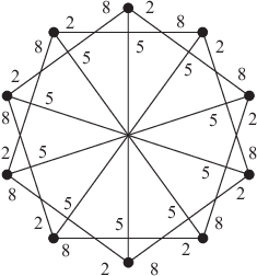
Before proceeding to our result in this section, we pause briefly to review some relevant definitions. Given a finite group and a set of generators , a Cayley graph is a graph whose vertices are the elements of the group () and whose edges correspond to the action of the generators (, where is the operation defined for ). We assume that the set of generators is closed under inversion, so is an undirected graph. A circulant graph (also known as a chordal ring) is a Cayley graph over , the cyclic group of order under the addition operation.
In [9], we have analyzed the class of regular graphs that admit an MCSD, and proved that this class is equivalent to that of circulant graphs. In this section, we prove that nearly all the cubic graphs in this class have a -CDC, the only exception being . We start by noting that a characterization of such cubic graphs follows directly from the results of [9] (specifically, Theorem 5, Lemma 6, and Lemma 7) and can be stated as follows.
Lemma 9.
admits an MCSD (or, equivalently, is a circulant graph) if and only if is isomorphic to either , with , or to , with .
We now present the main result of this section.
Theorem 10.
Except for , every cubic graph that admits an MCSD has a -CDC.
Proof.
By Lemma 9, it suffices to consider instances of , with , and of , with .
First, notice that all instances of or have girth less than . Also, the only instances of girth are and . The former of these is isomorphic to and obviously does not have a -CDC. As for the latter, a -CDC is shown in Figure 2(a).
Let us then consider the girth- instances; we do this by resorting to the material of Section 4.2. First notice that is isomorphic to and that all instances of , for , can be generated by successive replacements of by in . Similarly, is isomorphic to and all instances of , for , can be generated by successive replacements of by in . It then follows that every instance of or having also has a -CDC. ∎
7 Conclusions
We have in this paper demonstrated how to generate all the cubic graphs that have a -CDC in a constructive manner. For an arbitrary cubic graph with vertices and girth , our method provides, at least in principle, a mechanism for checking whether has a -CDC: one simply generates all girth- cubic graphs on vertices that have a -CDC and checks each one against for isomorphism. This check, we recall, can be performed polynomially for cubic graphs [10].
Our method also provides a mechanism for pinpointing a Hamiltonian cycle in any cubic graph that has a -CDC. That all such graphs are Hamiltonian is a result consistent with the one in [9], given our further demonstration, in this paper, that all non- cubic graphs that have an MCSD also have a -CDC. The alluded result in [9] is that all regular graphs that have an MCSD are Hamiltonian.
Our results relating -CDC’s to MCSD’s in cubic graphs create a bridge connecting these two concepts and also, by consequence, the notion of a circulant graph in the cubic case. The obvious implication of this is that results obtained within one context can now be extended directly to any other.
There are several open problems that may be addressed to expand on the results we have presented. Some of them come from generalizing the vertices’ fixed degree or the constant length of a CDC’s cycles, or yet from relaxing at least one of the two constraints by letting vertices have different degrees or CDC cycles different lengths. Relaxing both is really tantamount to addressing the Szekeres-Seymour conjecture [13, 12], according to which every -edge-connected graph has a CDC. This conjecture has stood for over thirty years, so perhaps an easier (though by no means trivial) starting problem for further research is to characterize the -regular graphs that have a -CDC, .
Acknowledgments
References
- [1] A. Altshuler. Construction and enumeration of regular maps on the torus. Discrete Mathematics, 4:201–217, 1973.
- [2] J. C. Bermond, F. Cornellas, and D. F. Hsu. Distributed loop computer networks: a survey. Journal of Parallel and Distributed Computing, 24:2–10, 1995.
- [3] J. A. Bondy and U. S. R. Murty. Graph Theory with Applications. North-Holland, New York, NY, 1976.
- [4] M. Deza, P. W. Fowler, A. Rassat, and K. M. Rogers. Fullerenes as tilings of surfaces. Journal of Chemical Information and Computer Sciences, 40:550–558, 2000.
- [5] P. Flocchini, B. Mans, and N. Santoro. On the impact of sense of direction on message complexity. Information Processing Letters, 63:23–31, 1997.
- [6] P. Flocchini, B. Mans, and N. Santoro. Sense of direction: definitions, properties and classes. Networks, 32:165–180, 1998.
- [7] P. Flocchini, B. Mans, and N. Santoro. Sense of direction in distributed computing. Theoretical Computer Science, 291:29–53, 2003.
- [8] E. C. Kirby, R. B. Mallion, and P. Pollack. Toroidal polyhexes. Journal of the Chemical Society Faraday Transactions, 89:1945–1953, 1993.
- [9] R. S. C. Leão and V. C. Barbosa. Minimal chordal sense of direction and circulant graphs. In R. Královič and P. Urzyczyn, editors, Mathematical Foundations of Computer Science 2006, volume 4162 of Lecture Notes in Computer Science, pages 670–680, Berlin, Germany, 2006. Springer-Verlag.
- [10] E. M. Luks. Isomorphism of graphs of bounded valence can be tested in polynomial time. Journal of Computer and System Sciences, 25:42–65, 1982.
- [11] N. Santoro. Sense of direction, topological awareness and communication complexity. SIGACT News, 2:50–56, 1984.
- [12] P. D. Seymour. Sums of circuits. In J. A. Bondy and U. S. R. Murty, editors, Graph Theory and Related Topics, pages 341–355. Academic Press, New York, NY, 1979.
- [13] G. Szekeres. Polyhedral decompositions of cubic graphs. Bulletin of the Australian Mathematical Society, 8:367–387, 1973.
- [14] C. Thomassen. Tilings of the torus and the Klein bottle and vertex-transitive graphs on a fixed surface. Transactions of the American Mathematical Society, 323:605–635, 1991.
- [15] C. Thomassen. Triangulating a surface with a prescribed graph. Journal of Combinatorial Theory, Series B, 57:196–206, 1993.