Automatic Verification of Timed Concurrent Constraint Programs

Automatic Verification of Timed Concurrent Constraint ProgramsThanks: This work has been partially supported by the EU (FEDER) and the Spanish MEC, under grant TIN 2004-7943-C04-02, by ICT for EU-India Cross Cultural Dissemination Project under grant ALA/95/23/2003/077-054, and by the Italian project Cofin’04 AIDA.

Moreno Falaschi
Dip. Matematica e Informatica University of Udine
Via delle Scienze 206. I-33100 Udine Italy
E-mail: falaschi@dimi.uniud.it
Alicia Villanueva
Dep. Sistemas Informáticos y Computación Technical University of Valencia
Camino de Vera s/n. E-46022 Valencia Spain
E-mail: villanue@dsic.upv.es

Revised 7 April 2004; Accepted 10 May 2005

Abstract

The language Timed Concurrent Constraint (tccp) is the extension over time of the Concurrent Constraint Programming (cc) paradigm that allows us to specify concurrent systems where timing is critical, for example reactive systems. Systems which may have an infinite number of states can be specified in tccp. Model checking is a technique which is able to verify finite-state systems with a huge number of states in an automatic way. In the last years several studies have investigated how to extend model checking techniques to systems with an infinite number of states. In this paper we propose an approach which exploits the computation model of tccp. Constraint based computations allow us to define a methodology for applying a model checking algorithm to (a class of) infinite-state systems. We extend the classical algorithm of model checking for LTL to a specific logic defined for the verification of tccp and to the tccp Structure which we define in this work for modeling the program behavior. We define a restriction on the time in order to get a finite model and then we develop some illustrative examples. To the best of our knowledge this is the first approach that defines a model checking methodology for tccp.

keywords

Automatic verification, reactive systems, timed concurrent constraint programming, model checking

1 Introduction

Model checking is a technique for formal verification that was defined for finite-state systems. It was first introduced in [10] and [30] for verifying automatically if a system satisfies a given property. Concurrent systems can be very complicated, and the process of modeling and verifying them by hand can be hard. Thus, the development of formal and fully automatic methods such as model checking is essential. Basically, this technique consists in an exhaustive analysis of the state-space of the system. This exhaustive analysis implies that, in principle, we can apply it only to finite-state systems limiting a lot its applicability. Furthermore, the state-explosion problem is the main drawback even for finite-state systems and for this reason many approaches in the literature try to mitigate it. Two of the main solutions for the state-explosion problem that have been presented in the last years are the symbolic approach [27] and the algorithms for abstract model checking [14]. The idea which is shared by these approaches is to reduce the number of states of the system.

The different approaches to the model checking problem for infinite state systems can be classified in two categories. The first one corresponds to those approaches that construct an abstract finite model of the system which can be automatically verified (see [11, 25]). The second category contains those approaches based on the symbolic reachability analysis where a finite representation of the set of reachable configurations of the system is calculated (see [2, 13, 8, 7]). The methodologies that make use of regular languages and regular relations are considered in the so called regular model checking approach [29, 24, 9]. Moreover, in [1] the notion of abstraction and the notion of symbolic reachability are combined in order to define a method to verify infinite-state systems. Our approach is novel and makes use of a notion of abstraction based on constraints and a time interval. The notion of constraints is used to collapse the number of states.

In [26] reactive systems are defined as those systems that keep exchanging information with their environment at run time. Reactive systems are typically defined as a set of processes working in parallel, hence the family of reactive systems is strictly related to the notion of concurrency. In some cases it is not expected that the system terminates but it may continue its execution indefinitely. Examples of such systems are operating systems, communication protocols or some kind of embedded systems. Thus it is quite useful to have a specification language that supports concurrency which makes easier for the user to describe systems. Usually, in model checking, by exploiting concurrency we model the whole system, including the environment. For example, users are represented as a concurrent process which models the possible actions that users can perform to interact with the system.

The language Temporal Concurrent Constraint Programming (tccp) extends the Concurrent Constraint Programming (cc) paradigm defined in [31] with a notion of time. This extension is suitable for modeling reactive systems. Actually, in the literature you can find two similar languages which extend cc with some notion of time: the tcc language first presented in [32] and the ntcc language defined in [28]. tccp is a declarative language defined in [4] that handles constraints which is a key characteristic for the results which we achieve in the present work. Our idea is to take advantage of the natural properties of the language in order to define a model-checking algorithm that allows us to verify reactive systems specified in tccp. Note that when we speak of reactive systems we are not limiting ourselves to finite-state systems. The tccp language allows us to model infinite-state systems, hence we tackle the problem of model checking for infinite-state systems. We show how the constraint nature of the language and the fact that it has a built-in notion of time can be exploited usefully.

Some related works can be found in the literature where constraints are used for solving similar problems. In [15, 16] the authors present a method that allows them to verify a communication protocol with an infinite number of states in the sense that they prove that a client-server protocol is correct for an arbitrary number of processes (clients). This could not be proved by using classical approaches to model checking, however it become possible thanks to the use of the notion of constraint.

The model-checking technique can be divided into three main phases; specification, modeling and verification. In this work, we use the notion of constraint in the three phases of the model-checking technique. First, we introduce the notion of constraint in the constructed model of the system. We note that constraints are able to represent in a compact manner a set of possible values that the system variables can take (i.e., a possibly infinite set of states if we use the classical notion of state). In the second phase we use a logic able to handle constraints for specifying the property to be verified. Such logic was presented in [5] and revisited in [6]. The last phase of the model-checking technique consists in defining an algorithm that determines whether the system satisfies the property by using the two outputs of the previous phases. In this work we extend the classical algorithm defined for LTL to the constrained approach. Note that we can take as a reference the classical algorithm because we use a logic able to handle constraints, and this makes possible to combine it with the tccp Structure defined in this paper to model the system. Since this structure contains constraints, it would not be possible to use a classical temporal logic directly. To the best of our knowledge this is the first time that a model-checking algorithm for systems specified with the tccp language is defined. Some of the results in this work have been included in Villanueva’s doctoral thesis [37].

In [18, 19] we presented a framework that allowed us to build a graph structure as a first step for applying the model-checking technique to tcc programs. tcc is a language similar to tccp for programming embedded systems. The main differences between tcc and the language that we consider here is in the deterministic nature of the tcc language versus the non-determinism, and the monotonicity of the store in tccp. Monotonicity means that the store of the system always increases. tcc is not monotonic since the store is reset when passing from one time instant to the following one. These differences make the graph structures defined in [18, 19] and in this work completely different. We will show these differences in detail in the following sections. Moreover, only the modeling process of the method was presented in [18, 19], whereas in this paper we provide the logic used for the specification of the property and the model-checking algorithm as well.

This paper is organized as follows. In Section 2 we introduce some basic theoretic notions. In Section 3 we present the basic notions of the tccp language. Then, in Section 4 we describe the method to construct an adequate model of the system, which is shown to model correctly the language operational semantics. In Section 5 we present the logic for specifying the properties of our system. In Section 6 we define the algorithm that applies the model-checking technique to this model and show its correctness. Section 7 discusses some related work. Finally, in Section 8 final remarks and future work are discussed.

2 Preliminaries

In this section we present some definitions necessary to follow the technical details of this work. For a quick reading it is possible to skip to Section 3.

A Constraint System is a system of partial information. We follow the definition of Saraswat et al.:

Definition 1 (Simple constraint system [34])

Let $D$ be a non-empty set of tokens or primitive constraints. A simple constraint system is a structure $\langle C,\vdash\rangle$ where $\vdash\subseteq\wp_{f}(C)\times C$ is an entailment relation satisfying:

C1: $u\vdash P$ whenever $P\in u$ ,
C2: $u\vdash Q$ whenever $u\vdash P$ for all $P\in v$ and $v\vdash Q$ .

Moreover, an element of $\wp_{f}(C)$ is called a finite constraint and $\vdash$ is extended to $\wp_{f}(C)\times\wp_{f}(C)$ in the obvious way. Finally, $u\approx v$ iff $u\vdash v$ and $v\vdash u$ . We also say that $u\geq v$ when $v\vdash u$ .

Definition 2 (Cylindric constraint system [34])

We define a cylindric constraint system as a structure $\langle C,\vdash,\mathcal{V},\{\exists_{x}\mid x\in\mathcal{V}\}\rangle$ such that $\langle C,\vdash\rangle$ is a simple constraint system, $\mathcal{V}$ is an infinite set of variables and, for each $x\in\mathcal{V}$ , $\exists_{x}:\wp_{f}(C)\rightarrow\wp_{f}(C)$ is an operation satisfying:

E1: $u\vdash\exists_{x}u$ ,
E2: $u\vdash v$ implies $\exists_{x}u\vdash\exists_{x}v$ ,
E3: $\exists_{x}(u\sqcup\exists_{x}v)\approx\exists_{x}u\sqcup\exists_{x}v$ ,
E4: $\exists_{x}\exists_{y}u\approx\exists_{y}\exists_{x}u$ .

$\exists_{x}$ is called the existential quantifier or cylindrification operator.

A set of diagonal elements for a cylindric constraint system is a family $\{\delta_{xy}\in C\mid x,y\in\mathcal{V}\}$ such that

D1: $\emptyset\vdash\delta_{xx}$ ,
D2: if $y\neq x,z$ then $\{\delta_{xz}\}\approx\exists_{y}\{\delta_{xy},\delta_{yz}\}$ ,
D3: if $x\neq y$ then $\{\delta_{xy}\}\sqcup\exists_{x}(u\sqcup\{\delta_{xy}\})\vdash u$ .

We define an element $c$ of a cylindric constraint system $\langle C,\vdash\rangle$ as a subset of $C$ closed by entailment, i.e., such that $u\subseteq_{f}c$ and $u\vdash P$ implies $P\in c$ .

3 Timed Concurrent Constraint Language

The tccp language was developed in [4]. It was designed as a computational model which allows one to model reactive and real-time systems. Thus, it is possible to specify and to verify distributed, concurrent systems where the notion of time is a crucial question. tccp is based on the cc paradigm [31, 33, 34] that was presented as a general concurrent computational model.

The computational model of cc is defined by means of a global store and a set of defined agents that can add (tell) information into the store or check (ask) whether a constraint is entailed by the store. Computations evolve as an accumulation of information into a global store. In tccp the agents defined for cc are inherited. The model is enriched with a new agent and a discrete global clock. It is assumed that ask and tell actions take one time-unit and the parallel operator is interpreted in terms of maximal parallelism. Computation evolves in steps of one time-unit. It is assumed that the response time of the constraint solver is constant, independently of the size of the store. In practice some restrictions (mentioned below) are taken in order to ensure that these hypothesis are reasonable (the reader can see [4] for details).

To model reactive systems it is necessary to have the ability to describe notions as timeout or preemption. The timeout behavior can be defined as the ability to wait for a specific signal and, if a limit of time is reached and such signal is not present, then an exception program is executed. The notion of preemption is the ability to abort a process when a specific signal is detected. In tccp these behaviors can be modeled by using the new conditional agent (not present in cc)

\mathsf{now}\,c\,\mathsf{then}\,A\,\mathsf{else}\,B

which tests if in the current time instant, the store entails the constraint $c$ and if it occurs, then in the same time instant it executes the agent $A$ ; otherwise, it executes $B$ (in the same time instant). A limit for the number of nested conditional agents is imposed in order to ensure the bounded time response of the constraint solver within a time instant.

3.1 Syntax

The tccp language is parametric to an underlying cylindric constraint system as defined in Section 2. Since now we assume that $\mathcal{C}\mathchar 61\relax\langle C,\vdash,\mathcal{V},\exists\rangle$ is the underlying constraint system for tccp. Given $\mathcal{C}$ , in Figure 1 we show the syntax of the agents of the language. We assume that $c$ and $c_{i}$ are finite constraints (i.e. elements) in $\mathcal{C}$ .

(Agents) A ::= $\mathsf{tell(}c\mathsf{)}$ – Tell $\mid$ $\mathsf{stop}$ – Stop $\mid$ $\sum_{i\mathchar 61\relax 1}^{n}\mathsf{ask(}c_{i}\mathsf{)}\rightarrow A_{i}$ – Choice $\mid$ $\mathsf{now}\,c\,\mathsf{then}\,A\,\mathsf{else}\,A$ – Conditional $\mid$ $A\mid\mid A$ – Parallel $\mid$ $\exists x\,A$ – Hiding $\mid$ $\mathsf{p(}x\mathsf{)}$ – Procedure Call (Declarations) D ::= $D\ldotp D$ $\mid$ $\mathsf{p(}x\mathsf{)}$ :- $A$ (Program) P ::= $D\ldotp A$

Figure 1: tccp syntax (following F. de Boer et al.)

The Parallel and Hiding agents are inherited from the cc model and behave in the same way. Thus, the Parallel agent represents concurrency, whereas the Hiding operator makes a variable local to some process. Also the Tell, Choice and Procedure Call agents were present in the cc model, but in tccp they have a different semantics since in the timed model, these three agents cause extension over time. The Tell agent adds the information $c$ to the store, but this information is available to other agents only in the following time instant. Therefore, we can say that the tell action takes one unit of time. The same thing occurs with the Choice and Procedure Call agents. Thus, when we execute the $\sum_{i\mathchar 61\relax 1}^{n}\mathsf{ask(}c_{i}\mathsf{)}\rightarrow A_{i}$ agent, the execution of $A_{i}$ starts in the next time instant. Note that the Choice agent models the nondeterministic behavior of the language, thus nondeterminism is always associated to a time delay.

Finally, the Conditional agent ( $\mathsf{now}\,c\,\mathsf{then}\,A\,\mathsf{else}\,B$ ) is the new agent introduced in the model in order to capture negative information. It behaves within a time unit in the sense that the condition is checked in the same instant of time as the execution of the corresponding agent is started. In particular, if the guard is satisfied, then $A$ will be executed, otherwise the agent $B$ will be executed (we note that $B$ is executed also in the case when the store entails neither $c$ nor $\neg c$ ). If we have two nested conditional agents, then the guards are recursively checked within the same time instant. This is the reason why tccp needs a restriction about the maximum number of nested conditional agents.

3.2 tccp Operational Semantics

In Figure 2 it is shown the operational semantics for tccp as described in [4]. Each transition step takes one unit of time. In a configuration ( $\mathbf{Conf}$ ) there are two components: a set of agents and a finite constraint representing the store. The transition relation $\longrightarrow\subseteq\mathbf{Conf}\times\mathbf{Conf}$ is the least relation that satisfies the rules in Figure 2. We can say that the transition relation characterizes the (temporal) evolution of the system.

R1 $\langle\mathsf{tell(}c\mathsf{)},d\rangle\longrightarrow\langle\mathsf{stop},c\sqcup d\rangle$ R2 $\langle\sum_{i\mathchar 61\relax 1}^{n}\mathsf{ask(}c_{i}\mathsf{)}\rightarrow A_{i},d\rangle\longrightarrow\langle A_{j},d\rangle$ $j\in[1,n]\;\mbox{and}\;d\vdash c_{j}$ R3 $\frac{\langle A,d\rangle\longrightarrow\langle A^{\prime},d^{\prime}\rangle}{\langle\mathsf{now}\,c\,\mathsf{then}\,A\,\mathsf{else}\,B,d\rangle\longrightarrow\langle A^{\prime},d^{\prime}\rangle}$ $d\vdash c$ R4 $\frac{\langle A,d\rangle\not\longrightarrow}{\langle\mathsf{now}\,c\,\mathsf{then}\,A\,\mathsf{else}\,B,d\rangle\longrightarrow\langle A,d\rangle}$ $d\vdash c$ R5 $\frac{\langle B,d\rangle\longrightarrow\langle B^{\prime},d^{\prime}\rangle}{\langle\mathsf{now}\,c\,\mathsf{then}\,A\,\mathsf{else}\,B,d\rangle\longrightarrow\langle B^{\prime},d^{\prime}\rangle}$ $d\not\vdash c$ R6 $\frac{\langle B,d\rangle\not\longrightarrow}{\langle\mathsf{now}\,c\,\mathsf{then}\,A\,\mathsf{else}\,B,d\rangle\longrightarrow\langle B,d\rangle}$ $d\not\vdash c$ R7 $\frac{\langle A,c\rangle\longrightarrow\langle A^{\prime},c^{\prime}\rangle\;\;\langle B,c\rangle\longrightarrow\langle B^{\prime},d^{\prime}\rangle}{\langle A\mid\mid B,c\rangle\longrightarrow\langle A^{\prime}\mid\mid B^{\prime},c^{\prime}\sqcup d^{\prime}\rangle}$ R8 $\frac{\langle A,c\rangle\longrightarrow\langle A^{\prime},c^{\prime}\rangle\;\;\langle B,c\rangle\not\longrightarrow}{\langle A\mid\mid B,c\rangle\longrightarrow\langle A^{\prime}\mid\mid B,c^{\prime}\rangle}$ R9 $\frac{\langle A,c\rangle\longrightarrow\langle A^{\prime},c^{\prime}\rangle\;\;\langle B,c\rangle\not\longrightarrow}{\langle B\mid\mid A,c\rangle\longrightarrow\langle B\mid\mid A^{\prime},c^{\prime}\rangle}$ R10 $\frac{\langle A,d\sqcup\exists_{x}c\rangle\longrightarrow\langle B,d^{\prime}\rangle}{\langle\exists^{d}xA,c\rangle\longrightarrow\langle\exists^{d^{\prime}}xB,c\sqcup\exists_{x}d^{\prime}\rangle}$ R11 $\langle\mathsf{p}(x),c\rangle\longrightarrow\langle A,c\rangle$ $\mathsf{p}(x):\mathchar 0\relax A\in D$

Figure 2: Operational semantics for tccp language extracted from F. de Boer et al.

Since tccp interprets concurrency in terms of maximal parallelism, we assume that there are as many processors as needed to execute a program. This behavior is described by means of rules R7, R8 and R9 where the reader can see that whenever it is possible, two agents are executed concurrently.

Rules R3, R4, R5 and R6 describe the operational semantics for the conditional agent. Note that the different possible behaviors depend on the store and on the initial configuration. Rule R10 shows the semantics for the Hiding operator. Intuitively, the rule says that, if there exists a transition $\langle A,d\sqcup\exists_{x}c\rangle\longrightarrow\langle B,d^{\prime}\rangle$ , then $d^{\prime}$ is the local information produced by $A$ ; moreover, this local information $d^{\prime}$ must be hidden from the main process.

The observable behavior of the language is defined from the transition system described in Figure 2 and considers the input/output of finite and infinite computations:

Definition 3 (Observable)

Let $A$ be an agent from the tccp language, the operational behavior is given by the set of resulting stores computed by $A$ for each given input store, considering finite and infinite computations.

\mathcal{O}(A)\mathchar 61\relax\{d\mid\langle A,c\rangle\longrightarrow\ldots\langle B,c_{i}\rangle\longrightarrow\ldots,\mbox{ where }d\equiv\{c,c_{1},\mathbin{\cdot}\mathbin{\cdot}\mathbin{\cdot},c_{i},\mathbin{\cdot}\mathbin{\cdot}\mathbin{\cdot}\}\}

3.3 Practical Example

We can find in the literature a variety of examples of systems that can be modeled using the tccp language. Here we develop a typical system: a microwave oven. In Figure 3 the reader can see the behavior of a microwave. We can note that, for example, if we are in a state where the door of the microwave is closed, the system is turned-off and no error is detected. If, from that state, we open the door, then we move to the state on the top of the figure.

Refer to caption — Figure 3: Example: the microwave system.

The whole system example is inspired in the system for a microwave control shown in the classical literature [12]. However, we have considered only a subpart of the system in order to easily use this example as a reference in this work. In Figure 4 we show the tccp program which models a reduced part of the microwave system. In particular, it models the part of the system which detects if the door is open when the microwave is turned-on.

$\mathsf{microwave\_error(}\mathrm{Door},\mathrm{Button},\mathrm{Error}\mathsf{)}$ :- $\exists\,D,B,E($ $\mathsf{tell(}\mathrm{Error}\mathchar 61\relax[\_|E]\mathsf{)}$ $||$ $(\mathsf{tell(}\mathrm{Door}\mathchar 61\relax[\_|D]\mathsf{)}$ $||$ $(\mathsf{tell(}\mathrm{Button}\mathchar 61\relax[\_|B]\mathsf{)}$ $||$ $(\mathsf{now}\,(\mathrm{Door}\mathchar 61\relax[\mathrm{open}\mid D]\wedge\mathrm{Button}\mathchar 61\relax[\mathrm{on}\mid B])\,\mathsf{then}$ $(\exists\,E1(\mathsf{tell(}\mathrm{E}\mathchar 61\relax[\mathrm{yes}\mid E1]\mathsf{)})||$ $\exists\,B1(\mathsf{tell(}B\mathchar 61\relax[\mathrm{off}\mid B1]\mathsf{)}))$ $\mathsf{else}$ $\exists\,E1(\mathsf{tell(}\mathrm{E}\mathchar 61\relax[\mathrm{no}\mid E1]\mathsf{)})||$ $\mathsf{microwave\_error(}D,B,E\mathsf{)}))))\mathbin{\cdot}$

Figure 4: Example of a tccp program: a simple error controller

Looking into the program code, we can observe that a Conditional agent checks if the door is open when the microwave is turned-on. In that case, it forces (with the Tell agent) that in the following time instant, the microwave is turned-off and an error signal is emitted. If it is not true that the door is open and the microwave is working on, then the program simply emits (via the Tell agent) a signal of no error that will be available in the global store in the following time instant. Therefore, this example corresponds to the part of the system which avoids wrong behaviors such as those in Figure 3 which are represented by the two states on the right.

This simple example allows us to illustrate the fact that tccp is not able to model strong preemption, i.e., it is not possible to turn-off the start button in the same instant when the error is detected. Actually, it is possible to start the execution of the agent that turns the button off, but the fact that it has been turned off is visible only in the following time instant.

4 tccp Model Checking

The cc paradigm has some interesting features which allow us to define a model-checking algorithm for reactive systems. We define a model-checking algorithm which uses a time interval (provided by the user) in order to restrict the state-space of the system in the cases when the algorithm does not terminates. The fact that the time is in the semantics makes reasonable the use of such restriction since the user knows how much time is needed to have a response from the system. The reader could think that the restriction to an interval of time could make the algorithm incomplete in too many cases. In the following sections we show that the time interval is not always used. Obviously, the user must provide a reasonable time interval. Moreover, if the limit is reached and the verification is terminated, then we obtain an over-approximation of the system thus some properties can still be checked. The idea to limit the verification to a time limit is not new. It has been used in different approaches, for example in [3].

Let us now develop a model-checking technique to tccp programs. The key ideas are that we use the notion of constraint which is underlying the language in order to have a compact model of the system first, and second, to handle the model directly to verify properties.

In the following we describe in detail the three main phases which implement the model-checking algorithm. We also illustrate each phase with the application of the method to the microwave example.

4.1 Model Construction

The first task of the method corresponds to the construction of the model of the system. In classical approaches, Kripke Structures¹¹ 1 Kripke Structures were defined in [23]. The definition can also be seen in [12] for example. are used to model the system behavior; in our approach we define a similar structure called tccp Structure whose states are essentially a conjunction of constraints of the underlying constraint system. The idea is to automatize the construction of the model of the system from the specification. In other words, we take a program written in tccp, and a model of the system behavior is constructed in an automatic way.

4.1.1 Program Labeling

First of all, we need a labeled version of the specification in order to construct the model of the system automatically. We adapt the idea introduced in [26] to our framework: a different label is assigned to each occurrence of an agent. Labels allow us to identify during the model construction in which point of the execution of the program we are. The presence or absence of a label determines if the associated agent can be executed or not during the computation. The labeling process consists on the introduction of a different label for each occurrence of a language construct:

Definition 4

Let $P$ be a specification, the labeled version $P_{l}$ of $P$ is defined as follows. The subindex $k\in\mathbb{N}$ corresponds to the number of labels introduced up to a given point. When the labeling process starts, $k\mathchar 61\relax 0$ and each time that we introduce a new fresh label, $k$ is incremented by one.

•

If $P\mathchar 61\relax\mathsf{stop}$ then $P_{l}\mathchar 61\relax l_{\mathsf{stop}_{k}}\mathsf{stop}$ .
•

If $P\mathchar 61\relax\mathsf{tell(}c\mathsf{)}$ then $P_{l}\mathchar 61\relax l_{\mathsf{tell}_{k}}\mathsf{tell(}c\mathsf{)}$ .
•

If $P\mathchar 61\relax\sum_{i\mathchar 61\relax 1}^{n}\mathsf{ask(}c_{i}\mathsf{)}\rightarrow A_{i}$ then $P_{l}\mathchar 61\relax l_{\mathsf{ask}_{k}}\sum_{i\mathchar 61\relax 1}^{n}\mathsf{ask(}c_{i}\mathsf{)}\rightarrow A_{l}$ .
•

If $P\mathchar 61\relax\mathsf{now}\,c\,\mathsf{then}\,A\,\mathsf{else}\,B$ then $P_{l}\mathchar 61\relax l_{\mathsf{now}_{k}}\mathsf{now}\,c\,\mathsf{then}\,A_{l}\,\mathsf{else}\,B_{l}$ .
•

If $P\mathchar 61\relax A||B$ then $P_{l}\mathchar 61\relax l_{||_{k}}(A_{l}||B_{l})$ .
•

If $P\mathchar 61\relax\exists x\,A$ then $P_{l}\mathchar 61\relax l_{e_{k}}\exists x\,A_{l}$ .
•

If $P\mathchar 61\relax\mathsf{p(}x\mathsf{)}$ then $P_{l}\mathchar 61\relax l_{\mathsf{p}_{k}}\mathsf{p(}x\mathsf{)}$ .

The labeling of a declaration $D$ of the form $\mathsf{p(}x\mathsf{)}$ :- $A$ is defined as $l_{\mathrm{p}_{i}}\mathsf{p(}x\mathsf{)}$ :- $A_{l}$ , called $D_{l}$ . Finally, the labeled version of a program of the form $D\ldotp A$ is $D_{l}\ldotp A_{l}$ .

In practice, we explore the tccp specification, and each time that we find an occurrence of a construct we introduce a new label which identifies such point of the program.

In Figure 5 we show the labeled version of the microwave error detection program showed in Figure 4. Note that the structure of the program has not changed, simply some labels have been added.

$\{l_{\mathrm{p}_{0}}\}\,\mathsf{microwave\_error(}\mathrm{Door},\mathrm{Button},\mathrm{Error}\mathsf{)}:\mathchar 0\relax$ $\{l_{\mathrm{e_{1}}}\}\,\exists\,D,B,E(\{l_{||_{2}}(\{l_{t_{3}}\}\mathsf{tell(}\mathrm{Error}\mathchar 61\relax[\_|E]\mathsf{)}||$ $(\{l_{\mathrm{||_{4}}}\}(\{l_{\mathrm{t_{5}}}\}\,\mathsf{tell(}\mathrm{Door}\mathchar 61\relax[\_|D]\mathsf{)}$ $||$ $\{l_{\mathrm{||_{6}}}\}(\{l_{t_{7}}\}\mathsf{tell(}\mathrm{Button}\mathchar 61\relax[\_|B]\mathsf{)}$ $||$ $\{l_{||_{8}}\}\,(\{l_{\mathrm{now}_{9}}\}\,\mathsf{now}\,(\mathrm{Door}\mathchar 61\relax[\mathrm{open}\mid D]\wedge\mathrm{Button}\mathchar 61\relax[\mathrm{on}\mid B])\,\mathsf{then}$ $\{l_{||_{10}}\}\,(\{l_{\mathrm{e_{11}}}\}\,\exists\,E1(\{l_{\mathrm{t_{12}}}\}\,\mathsf{tell(}\mathrm{E}\mathchar 61\relax[\mathrm{yes}\mid E1]\mathsf{)})||$ $\{l_{\mathrm{e_{13}}}\}\,\exists\,B1(\{l_{\mathrm{t_{14}}}\}\,\mathsf{tell(}B\mathchar 61\relax[\mathrm{off}\mid B1]\mathsf{)}))$ $\mathsf{else}$ $\{l_{\mathrm{e_{15}}}\}\,\exists\,E1(\{l_{\mathrm{t_{16}}}\}\,\mathsf{tell(}E\mathchar 61\relax[\mathrm{no}\mid E1]\mathsf{)})||$ $\{l_{\mathrm{p}_{17}}\}\,\mathsf{microwave\_error(}D,B,E\mathsf{)}))))\mathbin{\cdot}$

Figure 5: Example of a labeled tccp program: a simple error controller

4.1.2 The tccp Structure

The main point in the modeling phase is the construction of the graph structure which represents the system behavior. We define a new graph structure to represent the system. The tccp Structure is defined as a variant of the Kripke Structure. Intuitively, a Kripke Structure is a finite graph structure where there could be many initial nodes and each node is always related to another one (or to itself). Moreover, each state has associated a set of atomic propositions which are true in such state.

The main difference between the two structures is that the definition of a state in the Kripke Structure follows the classical notion of state whereas in our structure, a state consists of a conjunction of constraints and intuitively it can be seen as a set of classical states.

Let us formally define our tccp Structure.

Definition 5

The set $AP$ of atomic propositions is defined as the set of elements²² 2 See the definition in Section 2. of the cylindric constraint system $\mathcal{C}$ of the tccp language.

In the rest of the paper we abuse of notation by identifying the meaning of the terms constraint, atomic proposition and element. Next we define what a state of the tccp Structure is:

Definition 6 (tccp State)

Let $AP$ be the atomic propositions in the tccp syntax and $L$ be the set of all labels generated during the labeling process described above. We define the set of states as $S\subseteq 2^{AP}\times 2^{L}\;$ .

Before the definition of the tccp Structure, we define the notion of equivalent states. For this, we need the classical notion of renaming of variables. Let $y_{1},\ldots,y_{n}$ be $n$ distinct variables. The substitution $\{x_{1}/y_{1},\ldots,x_{n}/y_{n}\}$ is a renaming.

Definition 7 (Equivalent States)

Given two tccp states $s$ and $s^{\prime}$ , we say that the two states are equivalent if:

•

the set of labels $l\subseteq L$ of $s$ and the set of labels $l^{\prime}\subseteq L$ coincide and,
•

there exists a renaming $\gamma$ of variables of the constraints in $s$ which makes them syntactically identical to the set of constraints of $s^{\prime}$

In Definition 8, we define the tccp Structure. Observe that the differences w.r.t. a Kripke Structure are the definition of state (in Definition 6) and the two labeling functions $C$ and $T$ which replace the labeling function $L$ of the classical Kripke Structure.

Definition 8 (tccp Structure)

Let $AP$ be a set of atomic propositions, we define a tccp Structure $M$ over $AP$ as a five tuple $M\mathchar 61\relax(S,S_{0},R,C,T)$ where

1.

$S$ is a finite set of states.
2.

$S_{0}\subseteq S$ is the set of initial states.
3.

$R\subseteq S\times S$ is a transition relation.
4.

$C:S\rightarrow 2^{AP}$ is the function that returns the set of atomic propositions in a given state.
5.

$T:S\rightarrow 2^{L}$ as the function that returns the set of labels in a given state.

We assume that a transition in the graph represents an increment of one time-unit in the system. Intuitively, $C$ labels a state with the set of constraints true in such state. In other words, this function represents the new information that we know in a specific instant. $T$ labels each state with the set of labels associated to agents that must be executed in the following time instant. In other words, $T$ represents the point of execution in each instant (or state).

When two states $s$ and $s^{\prime}$ are related by $R(s,s^{\prime})$ , it means that it is possible to reach the state $s^{\prime}$ from state $s$ by executing the agents associated to the labels in $T(s)$ with the store $C(s)$ deriving as a result (by applying the renaming $\gamma$ ) the store $C(s^{\prime})$ and the point of execution $T(s^{\prime})$ . In other words, given a state $s$ and a renaming $\gamma$ , we obtain a state $s^{\prime}$ whose store is $C(s^{\prime})\cdot\gamma$ .

Given a tccp Structure $Z\mathchar 61\relax(S,S_{0},R,C,T)$ , we define $\mathop{tr(Z)}$ as the set of sequences of states of $Z$ starting from an initial state and which are related by $R$ :

\mathop{tr}(Z)\mathchar 61\relax\{s\mid s\mathchar 61\relax s_{0}\cdot s_{1}\cdots s_{n}\cdots\;\wedge s_{0}\in S_{0}\wedge\forall i\geq 0,\exists R(s_{i},s_{i\mathchar 43\relax 1})\}

(1)

Which intuitively means that for each $s_{i}$ , there exists a transition to the (renamed) state $s_{i\mathchar 43\relax 1}\cdot\gamma_{i}$ .

4.1.3 Construction of the model

In this section we show how the tccp Structure that represents the system behavior is constructed from a labeled specification $S$ in an automatic way. We present the pseudo-code of the necessary algorithms for the construction. Moreover, we show the complexity of such algorithms and explain the process from a theoretical point of view.

Intuitively, the construction evolves as follows. A process is composed by a set of clauses and a goal. A specification is a set of clauses. We describe how a specification (or declaration) can be transformed in a set of tccp Structures. Actually, for each different clause we construct a tccp Structure which is labeled with a unique name. This name can be used as one of the labels introduced in the program and is used when a procedure call refers to such clause. We consider that the declaration $D_{l}$ of the form $\mathsf{p(}x\mathsf{)}_{l}$ :- $A_{l}$ is a public information which is always available. We also assume that each label $l_{A}$ is associated with the agent $A$ .

The first algorithm that we show is the main procedure construct( $D$ ) (Figure 6) which, given a tccp declaration $D_{l}$ of the form $l_{p}\mathsf{p(}x\mathsf{)}:\mathchar 0\relax A_{l}$ , returns a tccp Structure $Q\mathchar 61\relax\langle S,S_{0},R,C,T\rangle$ representing the behavior of p.

We define globally a data type called state which represents a state of the tccp Structure. We assume that store is a conjunction of constraints and label is a set of labels in $L$ .

state :
	st : store;
	$\ell$ [ ] : label;

In our pseudo-code, we use the dot notation to access to the components of a state. Moreover, we use the notation $[\,]$ for lists of elements, thus $\ell[\,]$ is a list of labels. The $\aleph$ value is a possible value of a store denoting unsatisfiability.

Finally, we simplify the treatment of functions $C$ and $T$ . Although we do not mention them in the algorithm itself, these functions correspond to the two components of the state structure of the algorithm. We also write $R(n,n^{\prime})$ to describe that nodes $n$ and $n^{\prime}$ are related.

$\mathsf{construct}(\mathit{input}\,D:\mathrm{\textsf{tccp}{}\,declaration},\mathit{output}\,\langle S,S_{0},R,C,T\rangle:\mathrm{\textsf{tccp}{}\,Structure})$ s : state; $S^{\prime}$ , $S^{\prime}_{0}$ : set of states; inf[ ] : store; lab[ ] : set of labels; j : int; $S^{\prime}$ = $\emptyset$ ; // $\emptyset$ denotes the empty set $S^{\prime}_{0}$ = $\emptyset$ ; inf = $\mathsf{instant(}\mathit{true},l_{A}\mathsf{)}$ ; // $l_{p}\mathsf{p(}x\mathsf{)}:\mathchar 0\relax A_{l}$ lab = $\mathsf{follows(}l_{A}\mathsf{)}$ ; for $j\mathchar 61\relax 1$ to $\mathsf{sizeof(}\mathrm{inf}\mathsf{)}$ if inf[j] $\mathchar 60\relax\mathchar 62\relax\aleph$ then $s\mathchar 61\relax\mathsf{create\_node(}\mathrm{inf[j]},\mathrm{lab[j]}\mathsf{)}$ ; $C(s)\mathchar 61\relax$ inf[j]; $L(s)$ = lab[j]; $S^{\prime}\mathchar 61\relax S^{\prime}\cup\{s\}$ ; $S_{0}^{\prime}\mathchar 61\relax S^{\prime}$ ; $\mathsf{construct\_ag(}S^{\prime},S_{0}^{\prime},R^{\prime},C^{\prime},T^{\prime}\mathsf{)}$ ; $S\mathchar 61\relax S^{\prime}$ ; $S_{0}\mathchar 61\relax S^{\prime}_{0}$ ; $R\mathchar 61\relax R^{\prime}$ ; $C\mathchar 61\relax C^{\prime}$ ; $T\mathchar 61\relax T^{\prime}$ ;

Figure 6: Description of the construction algorithm

Roughly speaking, in this algorithm the tccp Structure is initialized and the set of initial states is created. Then the function construct_ag (Figure 7) is called. This function iteratively completes the construction. Functions instant and follows are two auxiliary procedures used during the construction of the tccp Structure. We show them below.

Now we show (Figure 7) the construct_ag procedure, which uses two more auxiliary functions: the $\mathsf{find(}s,S\mathsf{)}$ function, which returns a reference to the state in $S$ which coincides (modulo renaming of variables) with $s$ , and the perm function which, given two states, returns the necessary renamings which make them equivalent.

$\mathsf{construct\_ag}(\mathit{input/output}\,S[\,]:\mathrm{state};\mathit{input}\,S_{0}[\,]:\mathrm{state}$ $\mathit{input/output}\,R:\mathrm{relation},C,T:\mathrm{function})$ stat1, stat2 : state; s[ ], acc[ ] : state inf[ ] : store; lab[ ] : set of labels; rn : renaming of variables; j,k : int; acc = $S$ ; j = 0; while acc $\mathchar 60\relax\mathchar 62\relax\emptyset$ do stat1 = $\mathsf{select(}\mathrm{acc}\mathsf{)}$ ; acc = $\mathsf{remove(}\mathrm{acc},\mathrm{stat1}\mathsf{)}$ ; inf = $\mathsf{instant(}\mathrm{stat1\ldotp st},\mathrm{stat1}\ldotp\ell\mathsf{)}$ ; lab = $\mathsf{follows(}\mathrm{stat1}\ldotp\ell\mathsf{)}$ ; for k=1 to $\mathsf{sizeof(}\mathrm{inf}\mathsf{)}$ if inf[k] $\mathchar 60\relax\mathchar 62\relax\aleph$ then $s[j]\mathchar 61\relax\mathsf{create\_node(}\mathrm{inf[k]},\mathrm{lab[k]}\mathsf{)}$ ; $\mathrm{stat2}\mathchar 61\relax\mathsf{find(}s[j],S\mathsf{)}$ ; if (stat2) then // there exists an equivalent state $rn\mathchar 61\relax\mathsf{perm(}s[j],stat2\mathsf{)}$ ; $R(\mathrm{stat1},rn,\mathrm{stat2})$ ; else $R(\mathrm{stat1},\{\},\mathrm{s[j]})$ ; j = j + 1; $S\mathchar 61\relax S\cup$ {s[j]}; acc = acc $\cup$ {s[j]}; $C[j]\mathchar 61\relax\mathrm{inf[k]}$ ; $L[j]\mathchar 61\relax\mathrm{lab[k]}$ ;

Figure 7: Description of the construction algorithm for agents

Given a label $\mathit{ll}$ , follows( $ll$ ) returns the list which contains the labels associated to the agents that must be analyzed in the following time instant. Each element of the list corresponds to a different possible behavior of the system. For example, in the case of a conditional agent, the initial part of the list corresponds to the possible behaviors when the guard of the agent is satisfied, and the final part of the list corresponds to the case when it is not satisfied. Therefore, if two or more conditional agents are nested, then all the possible behaviors depending on the first then part will appear before those of the else part in the list. Since tccp restricts the number of nested conditional agents in a program, we can ensure that this algorithm terminates and the list of sets of labels is finite.

$\mathrm{list\_of\_sets\_of\_stores}\;\mathsf{follows}(ll:\mathrm{label})$ $\ell[],\ell_{1}[],\ell_{2}[]:\mathrm{set\_of\_labels};$ n, i, j : int; case $A$ of // we assume that $A$ is the agent associated with $ll$ . $\mathsf{stop}:\ell[1]\mathchar 61\relax\{\}$ ; $\mathsf{tell(}c\mathsf{)}:\ell[1]\mathchar 61\relax\{\}$ ; $\sum^{n}_{i\mathchar 61\relax 1}\mathsf{ask(}c_{i}\mathsf{)}\rightarrow A_{i}$ : for $j\mathchar 61\relax 1$ to $n$ $\ell[j]\mathchar 61\relax l_{A_{j}}$ ; $\ell[n\mathchar 43\relax 1]\mathchar 61\relax\{ll\}$ ; $\mathsf{now}\,c\,\mathsf{then}\,B_{1}\,\mathsf{else}\,B_{2}$ : $\ell_{1}\mathchar 61\relax\mathsf{follows}(l_{B_{1}})$ ; $\ell_{2}\mathchar 61\relax\mathsf{follows}(l_{B_{2}})$ ; $\ell\mathchar 61\relax\mathsf{append(}\ell_{1},\ell_{2}\mathsf{)}$ ; $B_{1}||B_{2}:\ell\mathchar 61\relax\mathsf{combine(}\mathsf{follows(}l_{B_{1}}\mathsf{)},\mathsf{follows(}l_{B_{2}}\mathsf{)}\mathsf{)};$ $\exists x\,B_{1}:\ell\mathchar 61\relax\mathsf{follows}(l_{B_{1}});$ $\mathsf{p(}x\mathsf{)}:\ell\mathchar 61\relax\{l_{p}\}$ ; // where $l_{p}$ represents the label // of the tccp Structure constructed for p $\mathsf{end\;case};$ return $\ell$ ;

Figure 8: Description of the auxiliary algorithm follows(

ll

)

The follows algorithm uses two additional auxiliary functions, append and combine, which are functions that implement operations over lists: $\mathsf{append(}\ell_{1},\ell_{2}\mathsf{)}$ returns the concatenation of the two lists $\ell_{1}$ and $\ell_{2}$ whereas $\mathsf{combine(}\ell_{1},\ell_{2}\mathsf{)}$ constructs a new list whose elements consist of an element of $\ell_{1}$ and an element of $\ell_{2}$ . For example, if $\ell_{1}\mathchar 61\relax\{\{l_{1}\},\{l_{2}\}\}$ and $\ell_{2}\mathchar 61\relax\{\{l_{3}\}\}$ , then the result of $\mathsf{combine(}\ell_{1},\ell_{2}\mathsf{)}$ is the list $\{\{l_{1},l_{3}\},\{l_{2},l_{3}\}\}$ .

We can show that the complexity of the algorithm showed in Figure 8 is exponential in the maximum number of nested agents in the specification. The high complexity is a theoretical case which does not occur in practice. We think that the complexity in practical cases should be semi-linear on average.

Lemma 1

The time complexity for the algorithm follows( $A$ ) presented in Figure 8 is $O(n*2^{m})$ where $m$ is the maximum number of nested agents and $n$ is the size of the list returned by follows( $A$ ).

Proof 4.1.

First of all, we know that the agent $A$ has a finite number of nested agents. Moreover, we can see that the cost of the algorithm in the case of Tell and Stop agents is constant since follows( $A$ ) = $\{\}$ in such cases. The cost is constant also in the case of Procedure Call agents since follows( $\mathsf{p(}x\mathsf{)}$ ) returns a single label. For the Choice agent, the cost depends on the number of asks contained in the agent. Therefore, given the agent $\sum^{n}_{i\mathchar 61\relax 1}\mathsf{ask(}c_{i}\mathsf{)}\rightarrow A_{i}$ , the cost will be $n\mathchar 43\relax 1$ . In addition, we know that the maximum number of nested recursive calls is $2^{m}$ which corresponds to the worst case: when every nested agent is a parallel or conditional agent. Note that in these cases, the functions combine or append are used. These are indeed the expensive operations which we count. We assume that the cost of these functions is linear in the size of the resulting list.

Thus, the time complexity of the worst case is $O(n*2^{m})$ .

Next we show the second auxiliary function needed during the automatic construction of the model (see Figure 9). Given a store and a label, instant( $c,ll$ ) returns a list of stores which corresponds to the information which can be computed instantaneously (i.e., before the following time instant) by executing the agents associated with the label $ll$ .

$\mathrm{list\_of\_stores}\;\mathsf{instant}(\mathit{input}\,\mathrm{st:store},ll:\mathrm{label})$ $s$ [], $s_{1}$ [], $s_{2}$ []: store; j: int; case $A$ of // we assume that $ll$ is associated to the agent $A$ $\mathsf{abort}:s[1]\mathchar 61\relax\mathit{true}$ ; $\mathsf{tell(}c\mathsf{)}:s[1]\mathchar 61\relax c$ ; $\sum^{n}_{i\mathchar 61\relax 1}\mathsf{ask(}d_{i}\mathsf{)}\rightarrow A_{i}$ : for $j\mathchar 61\relax 1$ to $n$ s[j] = { $d_{i}$ }; s[n+1] = $\mathit{true}$ ; $\mathsf{now}\,d\,\mathsf{then}\,B_{1}\,\mathsf{else}\,B_{2}$ : $s_{1}$ = $\mathsf{flat(}st,\mathsf{instant(}st\sqcup d,l_{B_{1}}\mathsf{)}\mathsf{)}$ ; $s_{2}\mathchar 61\relax\mathsf{flat(}st,\mathsf{instant(}\mathsf{not^{*}}(d)\sqcup st,l_{B_{2}}\mathsf{)}\mathsf{)}$ ; $s\mathchar 61\relax\mathsf{append(}s_{1},s_{2}\mathsf{)}$ ; $B_{1}||B_{2}:s\mathchar 61\relax\mathsf{combine(}\mathsf{instant(}st,l_{B_{1}}\mathsf{)},\mathsf{instant(}st,l_{B_{2}}\mathsf{)}\mathsf{)}$ $\exists x\,B_{1}:s[1]\mathchar 61\relax\{st[y/x]\}\sqcup\mathsf{instant(}st,l_{B_{1}}\mathsf{)}$ //where $y$ is a fresh variable $\mathsf{p(}x\mathsf{)}:s[1]\mathchar 61\relax\mathit{true}$ ; // where $\mathsf{p(}x\mathsf{)}::\{l_{B_{1}}\}B_{1}$ is a // clause of the specification $\mathsf{end\;case};$ return $s$ ;

Figure 9: Description of the auxiliary algorithm instant(

st,ll

)

In this algorithm we have marked the negation $\mathsf{not(c)}$ with a star to indicate that the semantics of negation is defined as the non satisfiability of $c$ instead of the satisfiability of $\neg c$ . The $\mathsf{instant}$ procedure uses the auxiliary function flat(st, $ll$ ) (Figure 10) which adds the constraint $st$ to each element of the list $ll$ returning a simple list of stores. If $st$ is inconsistent with any element of the list, then the value of the element is set to $\aleph$ .

$\mathrm{list\_of\_stores}\;\mathsf{flat}(\mathit{input}\,\mathrm{st:store},ll[]:\mathrm{store})$ s[]: store; j: int; for j = 1 to $\mathsf{sizeof(}ll\mathsf{)}$ if ll[j] $\sqcup$ st = $\mathit{false}$ then s[j] = $\aleph$ ; else s[j] = ll[j] $\sqcup$ st; return $s$ ;

Figure 10: Description of the auxiliary algorithm flat(st,

ll

)

It is easy to see that the time complexity of flat is linear on the size of the list.

Lemma 4.2.

The time complexity for the algorithm flat(c, $ll$ ) presented in Figure 10 is $O(n)$ where $n$ is the number of elements in the list $ll$ .

Proof 4.3.

The proof is trivial since we iterate $n$ times over the elements of the list.

The complexity of the algorithm instant showed above is exponential in the maximum number of nested agents in the specification. Note that also in this case, this is a theoretical case which may only occur very rarely in practice. We think that the complexity in practical cases should be semi-linear on average.

Lemma 4.4.

The time complexity for the algorithm instant(st, $A$ ) presented in Figure 9 is $O(n*2^{m}\mathchar 43\relax 2n)$ where $m$ is the maximum number of nested agents and $n$ is the cardinality of the list of stores returned by instant(st, $A$ ).

Proof 4.5.

We know that the agent $A$ has a finite number of nested agents. We also know that if the agent is a Stop, Tell or Procedure Call agent, then the cost of the function is constant. If $A$ is a Choice agent, then we have a linear cost, in particular we have $O(n\mathchar 43\relax 1)$ since there is an iterative loop over the number $n$ of guards in the Choice.

Now let us consider the three remaining cases. For both the Conditional and the Parallel agents we have two recursive calls, whereas for the Hiding agent we have a single recursive call. We assume that the combine and append functions are linear in the size of the two lists passed as argument (i.e., we take $O(n)$ where $n$ is the number of elements in the resulting list).

Therefore, we can say that the upper-bound for the global complexity of the algorithm is $O(n*2^{m}\mathchar 43\relax 2n)$ where $m$ is the maximum number of nested agents.

Now we can analyze the complexity of the construct algorithm. First of all, we state the complexity for the construct_ag function.

Lemma 4.6.

The time complexity for the algorithm construct_ag( $S,S_{0},s,R,C,T$ ) presented in Figure 7 is $O(c*m*2^{m})$ where $m$ is the maximum number of nested agents, and $c$ is the number of states in the model.

Proof 4.7.

By Lemma 4.4 and Lemma 1 we know the complexity of the auxiliary functions. Moreover, we know that select and remove take linear time and we assume that create_node has constant complexity. We know that the while loop will be executed $c$ times, where $c$ is the number of different states in the model.

We can see that each time the loop is executed, we have one procedure call to each auxiliary function. Moreover, we have a for loop which is executed at most $m\mathchar 43\relax 1$ times. Therefore, the cost of the for loop is $O(m)$ and the cost of the while loop is $2c*(m*2^{m})$ . We ensure the finiteness of the number of states since we know that there is a finite number of combinations of labels and constraints (which appear in the specification) modulo renaming.

Theorem 4.8.

The time complexity for the algorithm construct( $D$ ) presented in Figure 6 is $O(c*(2m*2^{m}))$ where $m$ is the maximum number of nested agents and $n$ is the cardinality of the resulting list.

Proof 4.9.

We know the cost of the auxiliary algorithms. Following the structure of the algorithm, we can see that there is one call to the construct_ag function. In addition, we have a procedure call to the algorithm instant and follows. Then, we have to add the cost of such algorithms: $O(2n*2^{m}\mathchar 43\relax c*(2m*2^{m}))$ . We have also a for loop which is executed at most $m$ times. Therefore, we obtain the global complexity given in this result.

Let us now explain intuitively the idea of algorithm showed in Figure 7. Each time an agent is analyzed, some actions are executed. In the following description we show the intuitions behind the formal definitions:

Stop: $S\equiv\mathsf{stop}$ . When we find a $\mathsf{stop}$ agent, we add no information to the store, insert a self-loop over the new node and instantiate the set of labels to the empty set since the construction must be concluded.
Tell: $S\equiv\mathsf{tell(}c\mathsf{)}$ . The new information $c$ is introduced into the store and the label associated to S is removed from the labels to be executed.
Choice: $S\equiv\sum^{n}_{i\mathchar 61\relax 1}\mathsf{ask(}c_{i}\mathsf{)}\rightarrow A_{i}$ . This agent leads to a set of corresponding branches in the graph. We introduce at most $m\mathchar 43\relax 1$ branches with $m\leq n$ , one for each possible successful ask guard. Note that if a $c_{i}$ condition is not consistent with the store $C(s)$ then the corresponding branch will not be generated. For each new node $s^{\prime}_{i}$ , we define the transition $R(s,s^{\prime}_{i}\cdot\gamma)$ where $\gamma$ is the renaming obtained when new nodes are generated, and we define an extra arc $R(s,s_{m\mathchar 43\relax 1}\cdot\gamma)$ that corresponds to the case when the store does not entail any condition $c_{i}$ but the execution of concurrent agents proceed (if there are no concurrent agents or there exist but they cannot proceed, then $s_{m\mathchar 43\relax 1}\mathchar 61\relax s$ thus a self-loop is introduced). Moreover, we do not introduce any additional information into the store and the labels are updated.
Conditional: $S\equiv\mathsf{now}\,c\,\mathsf{then}\,A\,\mathsf{else}\,B$ . The construction process in this case follows the same idea as for the choice operator: we define two new nodes ( $s^{\prime}_{1}$ and $s^{\prime}_{2}$ ) that correspond to the two possible behaviors. The first branch corresponds to the case when the store entails $c$ . It is added to the store the information that the agent $A$ can generate in a single time instant. Also the set of labels is updated. The second branch is defined in a similar way.
Parallel: $S\equiv A||B$ . When a parallel agent is analyzed, the new node generated depends on the execution of the agents $A$ and $B$ in the present time instant. This means that the new store is defined as the union of the information obtained from the execution of $A$ and $B$ (if it is possible to execute them). Also the set of labels depends on these two agents.
Hiding: $S\equiv\exists x\,A$ . The behavior of the hiding agent is modeled in the graph construction by the introduction of the necessary renaming of variables in the store.
Procedure Call: $S\equiv\mathsf{p(}X_{1},\ldots,X_{n}\mathsf{)}$ . When a procedure call is reached we finish the process by introducing in $s^{\prime}$ a reference to the initial node of the tccp Structure for $\mathsf{p}$ . If there are more concurrent agents that must be analyzed, then we continue by considering the tccp Structure already generated for such clause (with the necessary renaming of variables). We link the current node $s$ with a simplified copy of this piece of structure. The simplification consists in eliminating the branches whose condition is inconsistent with the constraints derived by the other (parallel) agents. Thus, the new node $s^{\prime}$ depends on the execution of the other concurrent agents and the body of the clause for $\mathsf{p}$ .

If there are two (or more) procedure calls in parallel the process is similar and as many nodes as different possible behaviors are generated.

In order to illustrate the construction process, in Figure 11 we present the construction of the tccp Structure for the program in Figure 5. Remember that this program simply detects if the door is open when the microwave works and in that case turns the system off and emits an error signal.

We can see how, for the first time instant, two nodes corresponding to the two possible behaviors of the conditional agent have been generated in the specification ( $\mathsf{n1}$ and $\mathsf{n2}$ ). Now look at the node $\mathsf{n1}$ where we have that $L(\mathsf{n1})\mathchar 61\relax\{\mathsf{lt3},\mathsf{lt12},\mathsf{lt5},\mathsf{lt7},\mathsf{lt14},\mathsf{lp17}\}$ . This means that in order to continue with the graph construction we have to try to execute the agents associated with such labels. The tell agents update the store with the information that an error combination has been encountered and in the next time instant a stop signal will be present. This is important because when we try to execute the procedure call associated with $\mathsf{lp}_{17}$ , only one of the two possible branches can be followed.

When we generate new nodes and the corresponding connecting arcs we should consider formulas which are renamed apart. Note that if we find a node equal (up to renaming) to another one, a loop will be formed in the graph and the construction following this branch will terminate.

Next we show an additional example which may be useful to understand the construction. Given the program

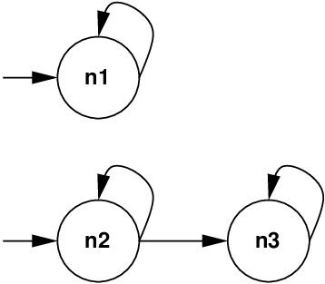
\mathsf{p(}x\mathsf{)}\mbox{:-}\exists y(\mathsf{tell(}x\mathchar 61\relax f(y)\mathsf{)}||p(y))

the constructed tccp Structure is shown in Figure 12. Note that, in each state, we store the new information added during a single time instant, thus the store of the program at a time instant $k$ is given by the union of the information added along the path in the structure, after making $k$ loops. For instance, after $3$ time instants, the derived information is the following: $\{x\mathchar 61\relax f(y),y\mathchar 61\relax f(y^{\prime})\}$ . Roughly speaking, each time we loop on the second node, a renaming of variables which form the constraints in the store is performed. Thus, the renaming $\{x/y,y/y^{\prime}\}$ where $y^{\prime}$ is a new variable, defines the new constraint $y\mathchar 61\relax f(y^{\prime})$ . Following the syntax of the program, $x\mathchar 61\relax f(y)$ and $y^{\prime}\mathchar 61\relax f(y^{\prime\prime})$ are introduced by the tell agent in the first and second time instant respectively. Note that we show the store after 3 instants of time since the information produced by a tell agent in a given time instant (for example, the second), does not appear in the store till the following time instant. This is due to the fact that tell agents take one time instant.

4.1.4 Correctness and Completeness

In this section we prove the correctness and completeness of the automatic construction of the model. We first introduce a function which extracts the information from the states of the tccp Structure. We define $\mathop{st}$ as the set of sequences of the form $\{t\mid t\mathchar 61\relax c_{1}\cdot c_{2}\cdots c_{n}\cdots\}$ where $c_{i}$ is a finite constraint.

Definition 4.10.

Given a tccp Structure $Z$ and $s\in tr(Z)$ of the form $s_{0}\cdot s_{1}\cdot\dots$ , we define the function $\delta_{s}:\mathop{tr(Z)}\rightarrow\mathop{st}$ as follows:

$\displaystyle\hskip 25.00003pt{\delta_{s}(s)\mathchar 61\relax\left\{\begin{array}[]{ll}C(s_{0})&\mbox{if $\mathop{s}\mathchar 61\relax s_{0}$,}\\ \delta(s_{0})\cdot\delta_{s}(s^{\prime})&\mbox{if $s\mathchar 61\relax s_{0}\cdot s^{\prime}$,}\end{array}\right\mathbin{\cdot}}$ where $\delta(s_{i})$ is defined as

$\displaystyle\hskip 25.00003pt{\delta(s_{i})\mathchar 61\relax\cup_{0\leq j\leq i}C(s_{j})}$

The extension of $\delta_{s}$ to sets of sequences is made in the obvious way.

The following theorem shows that the defined graph construction is correct and complete. In other terms it shows that the set of traces which correspond to the tccp structure $Z$ is the same given by the operational semantics of the tccp specification $S$ .

Theorem 4.11.

Let $Z$ be the tccp Structure corresponding to the tccp specification $S$ . Then the construction $Z$ is correct and complete since

$\delta_{s}(tr(Z))\mathchar 61\relax\mathcal{O}(S)$

Proof 4.12.

Let us first define an equivalence relation $\sim$ between configurations of the operational semantics presented in Figure 2 and graph states. Let $\sigma(\Gamma)$ be the store in configuration $\Gamma$ , then we extend $\sigma$ over sequences of configurations in the obvious way. In the graph, stores are ‘extracted’ by using function $C$ . Then, we say that a configuration $\Gamma$ corresponds to a tccp state $s$ if $C(s)\vdash\sigma(\Gamma)$ and $\sigma(\Gamma)\vdash C(s)$ , and the ‘active agent’ (namely one agent immediately reducible given the store in the current configuration) in $\Gamma$ corresponds to that selected for reduction in $s$ ; we denote this by $\Gamma\sim s$ .

A trace $t$ of the form $s_{0},\ldots,s_{i},\ldots$ in a tccp Structure $Z$ and a derivation (trace) $\gamma\mathchar 61\relax\gamma_{0},\ldots,\gamma_{i},\ldots$ in the operational semantics of a specification $S$ correspond iff $\delta_{s}(t)\mathchar 61\relax\gamma$ , i.e., $\forall i$ $\delta(s_{i})\sim\gamma_{i}$ . We must prove that all (the partial) paths in the tccp Structure $Z$ generated from the specification $S$ have an equivalent trace in the operational semantics of $S$ and vice-versa.

Let us first prove that $\delta_{s}(tr(Z))\subseteq\mathcal{O}(S)$ .

We proceed by induction on the length of the partial trace $n$ in $Z$ and on the structure of the agent $A$ selected in step $n$ . Note that each node in the tccp Structure has a finite number of successors, thus we can reason about all of them.

The basic case for $n\mathchar 61\relax 0$ is trivial, since the tccp Structure $Z$ is based on the same initial state $s_{0}$ considered in the operational semantics. Let us consider the inductive case, i.e., $n\mathchar 62\relax 0$ . Thus, let us consider the trace $s_{0},\ldots,s_{n}$ in $Z$ . We assume, by inductive hypothesis, that there exists a corresponding partial derivation $\gamma_{0},\ldots,\gamma_{n}$ in $\mathcal{O}(S)$ . We now prove that, if a further step is made in $Z$ starting from $s_{n}$ , it is possible to make a further step starting from $\gamma_{n}$ in $\mathcal{O}(S)$ and the new states still correspond. Let $\pi\mathchar 61\relax s_{0},\ldots,s_{n}\in\mathop{tr}(Z)$ and let $A$ be the active agent selected in $s_{n}$ . We have to consider several cases corresponding to the possible structure of $A$ .

Tell: $A\mathchar 61\relax\mathsf{tell(}c\mathsf{)}$ . Let $C(s_{n})\mathchar 61\relax d$ and $T(s_{n})\mathchar 61\relax\{l_{tell}\}$ . Then, we have the trace $\gamma\in\mathcal{O}(A)$ with $\gamma\mathchar 61\relax\gamma_{0},\gamma_{1},\ldots,\gamma_{n}$ and $\gamma_{n}\mathchar 61\relax\langle A,d\rangle$ , where $s_{n}$ and $\gamma_{n}$ correspond by inductive hypothesis. By the definition of the construction of the structure and the operational semantics we have that $C(s_{n\mathchar 43\relax 1})\mathchar 61\relax\{c\sqcup d\}$ , $T(s_{n\mathchar 43\relax 1})\mathchar 61\relax\{\}$ and $\gamma_{n\mathchar 43\relax 1}\mathchar 61\relax\langle\emptyset,c\sqcup d\rangle$ which correspond, thus $s_{n\mathchar 43\relax 1}\sim\gamma_{n\mathchar 43\relax 1}$ .
Choice: $A\mathchar 61\relax\sum^{m}_{i\mathchar 61\relax 1}\mathsf{ask(}c_{i}\mathsf{)}\rightarrow A_{i}$ . Let $C(s_{n})\mathchar 61\relax d$ and $T(s_{n})\mathchar 61\relax\{l_{\mathrm{ask}}\}$ . Then, we have the trace $\gamma\in\mathcal{O}(A)$ with $\gamma\mathchar 61\relax\gamma_{0},\gamma_{1},\ldots,\gamma_{n}$ and $\gamma_{n}\mathchar 61\relax\langle A,d\rangle$ . By inductive hypothesis we have that $s_{n}\sim\gamma_{n}$ . By definition of the construction of the structure and the operational semantics we have two cases: the first case is when there is no $c_{i}$ such that $d\vdash c_{i}$ , then in the construction of the tccp Structure there will be a loop, thus the state $s_{n\mathchar 43\relax 1}$ actually is the state $s_{n}$ whereas in the operational semantics there is no possible transition. In this case we just take $\gamma_{n\mathchar 43\relax 1}\mathchar 61\relax\gamma_{n}$ , and clearly $s_{n\mathchar 43\relax 1}\sim\gamma_{n\mathchar 43\relax 1}$ .

The second case is when there exists a $c_{i}$ such that $d\vdash c_{i}$ . This means that we have $C(s_{n\mathchar 43\relax 1})\mathchar 61\relax\{d\}$ and $T(s_{n\mathchar 43\relax 1})\mathchar 61\relax\{l_{A_{i}}\}$ . It is clear that by selecting $A$ in $\gamma_{n}$ , we derive $\gamma_{n\mathchar 43\relax 1}$ , which corresponds to $s_{n\mathchar 43\relax 1}$ .
Conditional: $A\mathchar 61\relax\mathsf{now}\,c\,\mathsf{then}\,A_{1}\,\mathsf{else}\,A_{2}$ . Let $C(s_{n})\mathchar 61\relax d$ and $T(s_{n})\mathchar 61\relax\{l_{\mathrm{now}}\}$ . Then, there exists a trace $\gamma\in\mathcal{O}(A)$ with $\gamma\mathchar 61\relax\gamma_{0},\gamma_{1},\ldots,\gamma_{n}$ and $\gamma_{n}\mathchar 61\relax\langle A,d\rangle$ , such that, by inductive hypothesis, $s_{n}\sim\gamma_{n}$ . By definition of the construction of the structure and the operational semantics we have two possible behaviors: either $d\vdash c$ or $d\not\vdash c$ . In the first case, $C(s_{n\mathchar 43\relax 1})\mathchar 61\relax\{d\sqcup\mathsf{instant(}d,l_{A_{n\mathchar 43\relax 1}}\mathsf{)}\}$ and $T(s_{n\mathchar 43\relax 1})\mathchar 61\relax\mathsf{follows}(A_{n\mathchar 43\relax 1})$ . On the other side, we have $\gamma_{n\mathchar 43\relax 1}\mathchar 61\relax\langle A_{1}^{\prime},d^{\prime}\rangle$ where $A_{1}^{\prime}$ is the agent reached by the execution of $A_{1}$ and $d^{\prime}$ the new store with the information added by the execution of $A_{1}$ . Clearly $s_{n\mathchar 43\relax 1}$ and $\gamma_{n\mathchar 43\relax 1}$ correspond. The case when $d\not\vdash c$ is similar, considering $A_{2}$ for reduction.
Parallel: $A\mathchar 61\relax A_{1}||A_{2}$ . Let $C(s_{n})\mathchar 61\relax d$ and $T(s_{n})\mathchar 61\relax\{l_{\mathrm{||}}\}$ . Then, we have the trace $\gamma\in\mathcal{O}(A)$ with $\gamma\mathchar 61\relax\gamma_{0},\gamma_{1},\ldots,\gamma_{n}$ and $\gamma_{n}\mathchar 61\relax\langle A,d\rangle$ . By inductive hypothesis $s_{n}\sim\gamma_{n}$ . By definition of the construction of the structure and the operational semantics we have that $C(s_{n\mathchar 43\relax 1})\mathchar 61\relax\{d\sqcup\mathsf{instant(}d,l_{A_{n\mathchar 43\relax 1}}\mathsf{)}\sqcup\mathsf{instant(}d,l_{A_{2}}\mathsf{)}\}$ and $T(s_{1})\mathchar 61\relax\{\mathsf{follows}(A_{1})\cup\mathsf{follows}(A_{2})\}$ . Then, we have $\gamma_{n\mathchar 43\relax 1}\mathchar 61\relax\langle A_{1}^{\prime}||A_{2}^{\prime},d^{\prime}\rangle$ where $A_{1}^{\prime}$ ( $A_{2}^{\prime}$ ) is the agent reached by the execution of $A_{1}$ ( $A_{2}$ ) and $d^{\prime}$ is the new store with the information added by the execution of $A_{1}$ and $A_{2}$ . Hence $s_{n\mathchar 43\relax 1}\sim\gamma_{n\mathchar 43\relax 1}$ .
Exists: $A\mathchar 61\relax\exists x\,A_{1}$ . Let $C(s_{n})\mathchar 61\relax d$ and $T(s_{n})\mathchar 61\relax\{l_{\mathrm{e}}\}$ . Then, we have the trace $\gamma\in\mathcal{O}(A)$ with $\gamma\mathchar 61\relax\gamma_{0},\gamma_{1},\ldots,\gamma_{n}$ and $\gamma_{n}\mathchar 61\relax\langle A,d\rangle$ . By inductive hypothesis $s_{n}\sim\gamma_{n}$ . We know that $C(s_{n\mathchar 43\relax 1})\mathchar 61\relax\{d\sqcup\mathsf{instant(}d,l_{A_{1}[y/x]}\mathsf{)}\}$ . Note that $\mathsf{instant(}d,l_{A_{1}[y/x]}\mathsf{)}$ represents the information generated in one time step by the agent $A_{1}[y/x]$ which is the result of the application of the substitution $y/x$ to the agent $A_{1}$ and $T(s_{n\mathchar 43\relax 1})\mathchar 61\relax\mathsf{follows}(A_{1})$ . $y$ is a fresh variable, thus the information generated by $A_{1}$ involving such variable will not affect the rest of the system.

Now, following the operational semantics we derive that $\gamma_{n\mathchar 43\relax 1}\mathchar 61\relax\langle\exists^{e^{\prime}}xB,d\sqcup\exists_{x}e^{\prime}\rangle$ , where $\langle A_{1},\exists_{x}d\rangle\rightarrow\langle B,e^{\prime}\rangle$ . Thus, we can identify $e^{\prime}$ with the information generated from agent $A_{1}$ , and $s_{n\mathchar 43\relax 1}$ and $\gamma_{n\mathchar 43\relax 1}$ correspond.
Procedure Call: $A\mathchar 61\relax\mathsf{p}(X)$ . Let $\mathsf{p(}X\mathsf{)}:\mathchar 0\relax B$ be a clause in the program (in the specification $S$ ). Let $C(s_{n})\mathchar 61\relax d$ and $T(s_{n})\mathchar 61\relax\{l_{p}\}$ . By inductive hypothesis, there exists the trace $\gamma\mathchar 61\relax\gamma_{0},\gamma_{1},\ldots,\gamma_{n}\in\mathcal{O}(A)$ and $\gamma_{n}\mathchar 61\relax\langle A,d\rangle$ . We have that $s_{n\mathchar 43\relax 1}\mathchar 61\relax N$ where $N$ is the first node of the tccp Structure constructed for $\mathsf{p(}X\mathsf{)}$ . We have that $C(s_{n\mathchar 43\relax 1})\mathchar 61\relax C(s_{n})$ and $T(s_{n\mathchar 43\relax 1})\mathchar 61\relax l_{B}$ . By expanding the procedure call in the operational semantics we get $\gamma_{n\mathchar 43\relax 1}\mathchar 61\relax\langle B,d\rangle$ , which clearly corresponds to $s_{n\mathchar 43\relax 1}$ .

Now we have to prove that $\mathcal{O}(S)\subseteq\delta_{s}(tr(Z))$ . This is completely analogous to the inclusion that we have proved.

5 Specification of the property

In this section we present the logic which we use in our model checking algorithm. This is a temporal logic which has also the ability to handle constraints of a given constraint system. In [5], the authors presented a temporal logic for reasoning about tccp programs. In particular, it is an epistemic logic with two modalities, one representing the knowledge and the other one representing the belief. These two modalities allow us to reason with the input-output behavior of programs.

Given an atomic proposition $c$ of the underlying constraint system, $\mathcal{K}(c)$ and $\mathcal{B}(c)$ are formulas of the logic which mean that $c$ is known or $c$ is belief respectively. In other words, $\mathcal{B}(c)$ holds if the process assumes that the environment provides $c$ whereas $\mathcal{K}(c)$ holds if the information $c$ is produced by the process itself.

The syntax of temporal formulas for this logic is shown below (see [5] for details):

Definition 5.13.

Given an underlying constraint system with set of constraints $\mathcal{C}$ , formulas of the temporal logic are defined by

\phi::\mathchar 61\relax\mathcal{K}(s)\mid\mathcal{B}(s)\mid\neg\phi\mid\phi\wedge\psi\mid\exists x\phi\mid\put(3.0,2.0){\circle{5.0}}\;\;\,\phi\mid\phi\,\mathcal{U}\,\psi

As for classical temporal logics, it is possible to define other logic operators such as the always or eventually operators from the basic ones. For example, if we want to express that a formula $\phi$ is satisfied at some point in the future, we write that $\Diamond\phi\mathchar 61\relax\mathit{true}\,\mathcal{U}\,\phi$ . To express that a formula $\phi$ is always satisfied, we can write that $\Box(\phi)\mathchar 61\relax\neg(\mathit{true}\,\mathcal{U}\,\neg\phi)$ . Moreover, as usual we denote by $\phi\rightarrow\psi$ the formula $\neg\phi\vee(\phi\wedge\psi)$ .

A reaction is defined as a pair of constraints of the form $\langle c,d\rangle$ where $c$ represents the input provided by the environment and $d$ corresponds to the information produced by the process itself. Moreover, it holds that $d\geq c$ for every reaction, i.e., the output always contains the input.

The truth value of temporal formulas is defined with respect to reactive sequences. $\langle c_{1},d_{1}\rangle\cdots\langle c_{n},d_{n}\rangle\langle d,d\rangle$ denotes a reactive sequence which consists of a sequence of reactions. Each reaction in the sequence represents a computation step performed by an agent at time $i$ . Intuitively each pair can be seen as the input-output behavior at time $i$ .

Therefore, given a reactive sequence $s$ we can define the truth values of formulas. The function $\mathsf{first}(s)$ returns the first reaction of a sequence, i.e., if $s\mathchar 61\relax\langle c_{1},d_{1}\rangle\cdots\langle c_{n},d_{n}\rangle\langle d,d\rangle$ then $\mathsf{first}(s)\mathchar 61\relax\langle c_{1},d_{1}\rangle$ . $\mathsf{next(}s\mathsf{)}$ returns the sequence obtained by removing the first reaction of it, i.e., if $s\mathchar 61\relax\langle c_{1},d_{1}\rangle\cdots\langle c_{n},d_{n}\rangle\langle d,d\rangle$ then $\mathsf{next}(s)\mathchar 61\relax\langle c_{2},d_{2}\rangle\cdots\langle c_{n},d_{n}\rangle\langle d,d\rangle$ .

We say that $\langle c,d\rangle\models\mathcal{B}(e)$ if $c\vdash e$ , i.e., the reaction “believes” the constraint $e$ if the first component of the reaction ( $c$ ) entails $e$ . Moreover, $\langle c,d\rangle\models\mathcal{K}(e)$ if $d\vdash e$ , i.e., the reaction $\langle c,d\rangle$ “knows” the constraint $e$ if its second component entails $e$ .

Definition 5.14 (by F. de Boer et al.).

Let $s$ be a timed reactive sequence and $\phi$ be a temporal formula. Then we define $s\models\phi$ by:

$\displaystyle\hskip 25.00003pt{\begin{array}[]{ll}s\models\mathcal{K}(c)&\mathrm{if}\hskip 14.22636pt\mathsf{first}(s)\models\mathcal{K}(c)\\ s\models\mathcal{B}(c)&\mathrm{if}\hskip 14.22636pt\mathsf{first}(s)\models\mathcal{B}(c)\\ s\models\neg\phi&\mathrm{if}\hskip 14.22636pts\not\models\phi\\ s\models\phi_{1}\wedge\phi_{2}&\mathrm{if}\hskip 14.22636pts\models\phi_{1}\mathrm{\;and\;}s\models\phi_{2}\\ s\models\exists x\phi&\mathrm{if}\hskip 14.22636pts^{\prime}\models\phi\mbox{ for some }s^{\prime}\;\mbox{such that}\;\exists_{x}s\mathchar 61\relax\exists_{x}s^{\prime}\\ s\models\put(3.0,2.0){\circle{5.0}}\;\;\,\phi&\mathrm{if}\hskip 14.22636pt\mathsf{next}(s)\models\phi\\ s\models\phi\mathcal{U}\psi&\mathrm{if}\hskip 14.22636pt\mathrm{for\;some}\;s^{\prime}\leq s,s^{\prime}\models\psi\;\mathrm{and\;for\;all\;}s^{\prime}\mathchar 60\relax s^{\prime\prime}\leq s,s^{\prime\prime}\models\phi\end{array}}$ where, for a sequence $s\mathchar 61\relax\langle c_{1},d_{1}\rangle\cdots\langle c_{n},d_{n}\rangle$ , we define the existential quantification $\exists_{x}s\mathchar 61\relax\langle\exists_{x}c_{1},\exists_{x}d_{1}\rangle\cdots\langle\exists_{x}c_{n},\exists_{x}d_{n}\rangle$ .

We say that a formula $\phi$ is valid ( $\models\phi$ ) if and only if for every reactive sequence $s$ , $s\models\phi$ holds. The reader can see that the modal operators $\mathcal{K}$ and $\mathcal{B}$ are monotonic w.r.t. the entailment relation of the underlying constraint system.

In this work we want to reason about tccp programs. Since the store of such programs evolves monotonically along the time, the notion of monotonically increasing reactive sequences is defined: let $s$ be a reactive sequence of the form $\langle c_{1},d_{1}\rangle\!\!\cdots\!\!\langle c_{n\mathchar 0\relax 1},d_{n\mathchar 0\relax 1}\rangle\langle c_{n},d_{n}\rangle$ , then we say that $s$ is monotonically increasing if it satisfies that $c_{i}\leq d_{i}$ and $d_{j}\leq c_{j\mathchar 43\relax 1}$ for each $i\in\{1,\ldots,n\}$ and $j\in\{1,\ldots,n\mathchar 0\relax 1\}$ . From now on we consider only monotonically increasing reactive sequences. In Table 1 some properties of the logic operators are shown.

Table 1: Logic Operators Properties

\mathcal{B}(c)\rightarrow\put(2.0,1.0){\line{1}{0}{4.0}}\put(6.0,1.0){\line{0}{1}{4.0}}\put(6.0,5.0){\line{-1}{0}{4.0}}\put(2.0,5.0){\line{0}{-1}{4.0}}\;\;\;(\mathcal{B}(c))

\mathcal{K}(c)\rightarrow\put(2.0,1.0){\line{1}{0}{4.0}}\put(6.0,1.0){\line{0}{1}{4.0}}\put(6.0,5.0){\line{-1}{0}{4.0}}\put(2.0,5.0){\line{0}{-1}{4.0}}\;\;\;(\mathcal{K}(c))

\mathcal{B}(c)\rightarrow\mathcal{K}(c)

\mathcal{K}(c)\rightarrow\put(3.0,2.0){\circle{5.0}}\;\;\,\mathcal{B}(c)

Therefore, whenever a constraint is believed in a specific time instant, then it will be believed also in all the following time instants. Moreover, if a given constraint is known at the present time instant, then it will be known at every time instant in the future.

Finally, we can define a relation between modal operators. In particular, we say that if a constraint $c$ is believed at a specific time instant, then it is also known. Also, if the constraint $c$ is known at a specific time instant, then it is believed at the following one.

The logic presented in this section can be seen as a kind of linear temporal logic. The reader can see that there are no quantifiers over alternative paths. It is considered that each instant of time has only one direct successor. If fact, if we compare this logic with the classical LTL logic (see [12] for example) we can see that each temporal operator corresponds to a temporal operator from LTL.

As we have said in the introduction, in model checking we assume a closed world in the sense that all the agents which can interact with the system are modeled. For this reason, the output in a time instant will always coincide with the input in the following time instant, i.e., it is not possible that other information different from the one generated by the model be introduced as an extra-input in any time instant. This mean that we can work with simple sequences of stores instead of working with sequences of reactions. We simply eliminate (or ignore) the second component of each reaction since it coincides with the fist one of the subsequent reaction.

¿From now, when we speak about sequences in the logic, we mean sequences of the form $s\mathchar 61\relax s_{0},s_{1},\ldots$ where each $s_{i}$ is a store and we omit the modal operator $\mathcal{K}$ . The monotonic properties described above are maintained.

5.1 Some examples

Here we illustrate which kind of properties we are able to specify using this logic. We refer to the program example in Figure 4. Remember that such example models a very simplified program which controls the state of the door of a microwave.

We could check if it is true that when an error is detected, then the microwave has been turned-off. Actually, the error has occurred in the previous time instant since the door was open and the microwave was working, but the program can emit the error signal only in the following time instant, and at the same time the microwave should be turned-off.

The following formula represents such property.

\begin{array}[]{ll}\neg(\mathit{true}\;\mathcal{U}\neg\exists_{\{\mathrm{Error,E,Button,B}\}}(&\mathrm{Error}\mathchar 61\relax[\mathrm{no}\mid E]\vee\\ &(\mathrm{Error}\mathchar 61\relax[\mathrm{yes}\mid E]\wedge\mathrm{Button}\mathchar 61\relax[\mathrm{off}\mid B])))\end{array}

(2)

It could seem that it is a complicate formula but if we think in terms of the always and eventually operators defined before, it becomes a very intuitive formula:

\Box\exists_{\{\mathrm{Error,E,Button,B}\}}(\mathrm{Error}\mathchar 61\relax[\mathrm{no}\mid E]\vee(\mathrm{Error}\mathchar 61\relax[\mathrm{yes}\mid E]\wedge\mathrm{Button}\mathchar 61\relax[\mathrm{off}\mid B]))

We can also model the property that the door will be eventually closed:

\Diamond\exists_{\{\mathrm{Door,D}\}}(\mathrm{Door}\mathchar 61\relax[\mathrm{close}\mid D])

(3)

Let us now remark the importance of the chosen logic in this work. We know that states of the tccp Structure represent only partial information. Therefore, if we want to check properties directly in the tccp Structure, then we need a logic able to handle partial information, as is the case of the logic presented in this section.

If we use any classical logic, we should consider each possible valuation of the variable values for each tccp state. In that case we had the same problem as in [18, 19], i.e., we would not take advantage of the compact representation of the system that constraints can provide. Finally, the model-checking algorithm would not be effectively applicable for the state-explosion problem.

6 The algorithm

The third and last phase of the model-checking technique is to define the algorithm which checks if a given temporal formula is satisfied by the model. The idea of the algorithm is similar to that for the classical tableau algorithm for the LTL model checking problem. The first thing is to construct the closure of the formula $\phi$ that we want to verify. Such closure is reminiscent of the Fischer-Ladner’s one [21].

Actually, if we intend to prove that the model satisfies the formula $\phi$ , then we construct the closure of the negated formula ( $\neg\phi$ ). The atomic propositions of the logic are those of the underlying constraint system. The closure of the negated formula and the tccp Structure are used to construct a graph structure (called the model-checking graph). This graph structure consists of nodes of the form $(q,\Phi)$ where $q$ is a state of the tccp Structure and $\Phi$ is a set of formulas from the closure of $\neg\phi$ . The constructed graph structure allows us to verify if the property is satisfied or not by the system by using well known graph algorithms. In particular, we look for a path which starts from an initial state and reaches a strongly connected component (SCC) which satisfies some properties. If such path exists, then we can say that the property $\neg\phi$ is satisfied, thus $\phi$ is not satisfied in the model of the system. In this section we describe this process more in detail.

The construction of the graph combining the formula and the model might not terminate. It is for this reason that we use the interval of time which the user provides to the system. This interval imposes a time limit. If such time limit is reached, the system aborts the construction of the graph. The idea is that if this occurs, then we have obtained an over-approximation of the model, which nevertheless allows us to make useful verifications over the finite graph calculated.

6.1 The closure of the formula

The closure $CL(\phi)$ of a formula $\phi$ allows us to determine its truth value. Intuitively, it is the set of sub-formulas that can affect the truth value. This set is used classically to define tableaux algorithms where sub-formulas are evaluated as follows: simplest formulas are evaluated first, then more complex formulas are considered. Thus, we can say that the closure of $\phi$ ( $CL(\phi)$ ) is the smallest set of formulas satisfying the following conditions:

•

$\phi\in CL(\phi)$ ,
•

$\neg\phi_{1}\in CL(\phi)$ iff $\phi_{1}\in CL(\phi)$ ,
•

if $\phi_{1}\wedge\phi_{2}\in CL(\phi)$ , then $\phi_{1},\phi_{2}\in CL(\phi)$ ,
•

if $\exists x\phi_{1}\in CL(\phi)$ , then $\phi_{1}\in CL(\phi)$ ,
•

if $\put(3.0,2.0){\circle{5.0}}\;\;\,\phi_{1}\in CL(\phi)$ , then $\phi_{1}\in CL(\phi)$ ,
•

if $\neg\put(3.0,2.0){\circle{5.0}}\;\;\,\phi_{1}\in CL(\phi)$ , then $\put(3.0,2.0){\circle{5.0}}\;\;\,\neg\phi_{1}\in CL(\phi)$ ,
•

if $\phi_{1}\mathcal{U}\phi_{2}\in CL(\phi)$ , then $\phi_{1},\phi_{2},\put(3.0,2.0){\circle{5.0}}\;\;\,\phi_{1}\mathcal{U}\phi_{2}\in CL(\phi)$ .

Note that in the case of $\neg\put(3.0,2.0){\circle{5.0}}\;\;\,\phi_{1}$ it is necessary to introduce the formula $\put(3.0,2.0){\circle{5.0}}\;\;\,\neg\phi_{1}$ which cannot be generated by the other rules.

Now we consider the microwave program example. The formula (2) for which we calculate the closure is that presented in the previous section.

Example 6.15.

For the program showed in Figure 4 we construct the closure of the formula which we want to verify, starting from the negation of Formula (2). Note that we assume that $\neg\neg\phi\mathchar 61\relax\phi$ . We also change in the obvious way the disjunction operator into a conjunction:

\mathit{true}\,\mathcal{U}\,(\neg(\textrm{Error=[no}\mid E])\wedge\neg(\textrm{Error=[yes}\mid E]\wedge\textrm{Button=[off}\mid B]))

(4)

Then, we show the closure of the formula. Note that the size of the set of formulas in the closure increases polynomially with the size of the formula (meaning the number of operators in the formula).

$\begin{array}[]{l}CL(\chi)\mathchar 61\relax\{\mathit{true}\,\mathcal{U}\,(\neg(\mathrm{Error}\mathchar 61\relax[\mathrm{no}\mid E])\wedge\neg(\mathrm{Error}\mathchar 61\relax[\mathrm{yes}\mid E]\wedge\mathrm{Button}\mathchar 61\relax[\mathrm{off}\mid B])),\\ \hskip 20.00003pt\mathit{true},\\ \hskip 20.00003pt\mathit{false},\\ \hskip 20.00003pt\neg(\mathrm{Error}\mathchar 61\relax[\mathrm{no}\mid E])\wedge\neg(\textrm{Error}\mathchar 61\relax[\mathrm{yes}\mid E]\wedge\mathrm{Button}\mathchar 61\relax[\mathrm{off}\mid B]),\\ \hskip 20.00003pt\neg(\mathrm{Error}\mathchar 61\relax[\mathrm{no}\mid E]),\\ \hskip 20.00003pt\neg(\textrm{Error}\mathchar 61\relax[\mathrm{yes}\mid E]\wedge\mathrm{Button}\mathchar 61\relax[\mathrm{off}\mid B]),\\ \hskip 20.00003pt\neg(\neg(\mathrm{Error}\mathchar 61\relax[\mathrm{no}\mid E])\wedge\neg(\textrm{Error}\mathchar 61\relax[\mathrm{yes}\mid E]\wedge\mathrm{Button}\mathchar 61\relax[\mathrm{off}\mid B])),\\ \hskip 20.00003pt\mathrm{Error}\mathchar 61\relax[\mathrm{no}\mid E],\\ \hskip 20.00003pt\mathrm{Error}\mathchar 61\relax[\mathrm{yes}\mid E]\wedge\mathrm{Button}\mathchar 61\relax[\mathrm{off}\mid B],\\ \hskip 20.00003pt\mathrm{Error}\mathchar 61\relax[\mathrm{yes}\mid E],\\ \hskip 20.00003pt\mathrm{Button}\mathchar 61\relax[\mathrm{off}\mid B],\\ \hskip 20.00003pt\neg(\mathrm{Error}\mathchar 61\relax[\mathrm{yes}\mid E]),\\ \hskip 20.00003pt\neg(\mathrm{Button}\mathchar 61\relax[\mathrm{off}\mid B]),\\ {\hskip 20.00003pt}\put(3.0,2.0){\circle{5.0}}\;\;\,\mathit{true}\,\mathcal{U}\,(\neg(\mathrm{Error}\mathchar 61\relax[\mathrm{no}\mid E])\wedge\neg(\mathrm{Error}\mathchar 61\relax[\mathrm{yes}\mid E]\wedge\mathrm{Button}\mathchar 61\relax[\mathrm{off}\mid B])),\\ \hskip 20.00003pt\neg(\put(3.0,2.0){\circle{5.0}}\;\;\,\mathit{true}\,\mathcal{U}\,(\neg(\mathrm{Error}\mathchar 61\relax[\mathrm{no}\mid E])\wedge\neg(\mathrm{Error}\mathchar 61\relax[\mathrm{yes}\mid E]\wedge\mathrm{Button}\mathchar 61\relax[\mathrm{off}\mid B]))),\\ {\hskip 20.00003pt}\put(3.0,2.0){\circle{5.0}}\;\;\,\neg(\mathit{true}\,\mathcal{U}\,(\neg(\mathrm{Error}\mathchar 61\relax[\mathrm{no}\mid E])\wedge\neg(\mathrm{Error}\mathchar 61\relax[\mathrm{yes}\mid E]\wedge\mathrm{Button}\mathchar 61\relax[\mathrm{off}\mid B]))),\\ \hskip 20.00003pt\neg(\mathit{true}\,\mathcal{U}\,(\neg(\mathrm{Error}\mathchar 61\relax[\mathrm{no}\mid E])\wedge\neg(\mathrm{Error}\mathchar 61\relax[\mathrm{yes}\mid E]\wedge\mathrm{Button}\mathchar 61\relax[\mathrm{off}\mid B])))\\ \hskip 20.00003pt\}\end{array}$

6.2 The model-checking graph

Given a formula $\phi$ of the logic described in Section 5, and the tccp Structure $Z$ constructed from the specification, the graph $G(\phi,Z)$ is defined as follows

Definition 6.16 (Model-Checking Graph).

Let $\phi$ be a formula, $CL(\phi)$ the closure of $\phi$ as defined in Section 6.1 and $Z$ the tccp Structure constructed following the algorithm described in Section 4.1.3. A node $n$ of the model-checking graph is formed by a pair of the form $(s_{n},\mathcal{Q}_{n})$ where $s_{n}$ is a state of $Z$ and $\mathcal{Q}_{n}$ is a subset of $CL(\phi)$ and the atomic propositions such that the following conditions are satisfied:

•

for each atomic proposition $p$ , $\mathcal{K}(p)\in\mathcal{Q}_{n}$ iff $p\in C(s_{n})$ ,
•

for every $\exists x\phi_{1}\in CL(\phi),\exists x\phi_{1}\in\mathcal{Q}_{n}$ iff $\exists_{x}\phi_{1}\in C(s_{n})$ ,
•

for every $\phi_{1}\in CL(\phi),\phi_{1}\in\mathcal{Q}_{n}$ iff $\neg\phi_{1}\not\in\mathcal{Q}_{n}$ ,
•

for every $\phi_{1}\wedge\phi_{2}\in CL(\phi),\phi_{1}\wedge\phi_{2}\in\mathcal{Q}_{n}$ iff $\phi_{1}\in\mathcal{Q}_{n}$ and $\phi_{2}\in\mathcal{Q}_{n}$ ,
•

for every $\neg\put(3.0,2.0){\circle{5.0}}\;\;\,\phi_{1}\in CL(\phi),\neg\put(3.0,2.0){\circle{5.0}}\;\;\,\phi_{1}\in\mathcal{Q}_{n}$ iff $\put(3.0,2.0){\circle{5.0}}\;\;\,\neg\phi_{1}\in\mathcal{Q}_{n}$ ,
•

for every $\phi_{1}\,\mathcal{U}\,\phi_{2}\in CL(\phi),\phi_{1}\,\mathcal{U}\,\phi_{2}\in\mathcal{Q}_{n}$ iff $\phi_{2}\in\mathcal{Q}_{n}$ or $\phi_{1},\put(3.0,2.0){\circle{5.0}}\;\;\,\phi_{1}\,\mathcal{U}\,\phi_{2}\in\mathcal{Q}_{n}$ .

An edge in the graph is defined as follows: there will be an edge from one node $n_{1}\mathchar 61\relax(s_{1},Q_{1})$ to another node $n_{2}\mathchar 61\relax(s_{2},Q_{2})$ iff there is an arc from the node $s_{1}$ to the node $s_{2}$ in the tccp Structure and for every formula $\put(3.0,2.0){\circle{5.0}}\;\;\,\phi_{1}\in CL(\phi)$ , $\put(3.0,2.0){\circle{5.0}}\;\;\,\phi_{1}\in Q_{1}$ iff $\phi_{1}\in Q_{2}$ .

Note that, in the definition above, when we take into consideration the set of arcs of the tccp Structure (when analyzing the formulas containing the next operator), we also consider the renaming that may label these arcs.

Intuitively, for each node of the model-checking graph, in $\mathcal{Q}$ we have the largest consistent set of formulas that is also consistent with the labelling function (the function $C$ ) of the tccp Structure. Moreover, two nodes of the graph are related if the temporal formulas in their $\mathcal{Q}$ sets are consistent.

For each node $s_{i}$ of the tccp Structure many nodes are generated in the model-checking graph. All these nodes have as first component the state $s_{i}$ and the second component consists of the different consistent sets of formulas derived from $C(s_{i})$ and the closure of the formula.

Next we show an example to illustrate how the nodes of the model-checking graph are constructed. We construct the graph for the negation of the property since we intend to prove that there is no computation of the system which satisfies the negated property. This is equivalent to prove that the property is satisfied for all the computations.

Example 6.17.

In this example we show some nodes of the graph which would result from our program example. We take the tccp Structure shown in Figure 11 and the closure set of the formula showed in the previous section.

Here we show two of the nodes generated for $s_{1}$ and one of the nodes generated for $s_{2}$ .

$\begin{array}[]{rl}n_{1}\mathchar 61\relax&(s_{1},Q_{1})\;\mathrm{where}\\ Q_{1}\mathchar 61\relax&\{\\ &\mathrm{Door}\mathchar 61\relax[\mathrm{open}\mid D]\wedge\mathrm{Button}\mathchar 61\relax[\mathrm{on}\mid B],\\ &\mathit{true},\;\mathrm{Error}\mathchar 61\relax[\mathrm{no}\mid E],\\ &\neg(\mathrm{Button}\mathchar 61\relax[\mathrm{off}\mid B]),\\ &\neg(\mathrm{Error}\mathchar 61\relax[\mathrm{yes}\mid E]\wedge\mathrm{Button}\mathchar 61\relax[\mathrm{off}\mid B]),\\ &\neg(\neg(\mathrm{Error}\mathchar 61\relax[\mathrm{no}\mid E])\wedge\neg(\mathrm{Error}\mathchar 61\relax[\mathrm{yes}\mid E]\wedge\mathrm{Button}\mathchar 61\relax[\mathrm{off}\mid B])),\\ &\put(3.0,2.0){\circle{5.0}}\;\;\,\mathit{true}\;\mathcal{U}\;(\neg(\mathrm{Error}\mathchar 61\relax[\mathrm{no}\mid E])\wedge\neg(\mathrm{Error}\mathchar 61\relax[\mathrm{yes}\mid E]\wedge\mathrm{Button}\mathchar 61\relax[\mathrm{off}\mid B])),\\ &\mathit{true}\;\mathcal{U}\;(\neg(\mathrm{Error}\mathchar 61\relax[\mathrm{no}\mid E])\wedge\neg(\mathrm{Error}\mathchar 61\relax[\mathrm{yes}\mid E]\wedge\mathrm{Button}\mathchar 61\relax[\mathrm{off}\mid B]))\\ &\}\end{array}$

$\begin{array}[]{rl}n_{2}\mathchar 61\relax&(s_{1},Q_{2})\;\mathrm{where}\\ Q_{2}\mathchar 61\relax&\{\\ &\mathrm{Door}\mathchar 61\relax[\mathrm{open}\mid D]\wedge\mathrm{Button}\mathchar 61\relax[\mathrm{on}\mid B],\\ &\mathit{true},\;\mathrm{Error}\mathchar 61\relax[\mathrm{yes}\mid E],\\ &\neg(\mathrm{Button}\mathchar 61\relax[\mathrm{off}\mid B]),\\ &\neg(\mathrm{Error}\mathchar 61\relax[\mathrm{yes}\mid E]\wedge\mathrm{Button}\mathchar 61\relax[\mathrm{off}\mid B]),\\ &\neg(\mathrm{Error}\mathchar 61\relax[\mathrm{no}\mid E])\wedge\neg(\mathrm{Error}\mathchar 61\relax[\mathrm{yes}\mid E]\wedge\mathrm{Button}\mathchar 61\relax[\mathrm{off}\mid B]),\\ &\mathit{true}\;\mathcal{U}\;(\neg(\mathrm{Error}\mathchar 61\relax[\mathrm{no}\mid E])\wedge\neg(\mathrm{Error}\mathchar 61\relax[\mathrm{yes}\mid E]\wedge\mathrm{Button}\mathchar 61\relax[\mathrm{off}\mid B])),\\ &\put(3.0,2.0){\circle{5.0}}\;\;\,\mathit{true}\;\mathcal{U}\;(\neg(\mathrm{Error}\mathchar 61\relax[\mathrm{no}\mid E])\wedge\neg(\mathrm{Error}\mathchar 61\relax[\mathrm{yes}\mid E]\wedge\mathrm{Button}\mathchar 61\relax[\mathrm{off}\mid B]))\\ &\}\end{array}$

$\begin{array}[]{rl}n_{3}\mathchar 61\relax&(s_{2},Q_{3})\;\mathrm{where}\\ Q_{3}\mathchar 61\relax&\{\\ &\mathrm{Error}\mathchar 61\relax[\mathrm{yes}\mid E],\;\mathrm{Button}\mathchar 61\relax[\mathrm{off}\mid B],\\ &\neg(\mathrm{Door}\mathchar 61\relax[\mathrm{open}\mid D]\wedge\mathrm{Button}\mathchar 61\relax[\mathrm{on}\mid B]),\\ &\mathit{true},\\ &\mathrm{Error}\mathchar 61\relax[\mathrm{yes}\mid E]\wedge\mathrm{Button}\mathchar 61\relax[\mathrm{off}\mid B],\\ &\neg(\neg(\mathrm{Error}\mathchar 61\relax[\mathrm{no}\mid E])\wedge\neg(\mathrm{Error}\mathchar 61\relax[\mathrm{yes}\mid E]\wedge\mathrm{Button}\mathchar 61\relax[\mathrm{off}\mid B])),\\ &\put(3.0,2.0){\circle{5.0}}\;\;\,\mathit{true}\;\mathcal{U}\;(\neg(\mathrm{Error}\mathchar 61\relax[\mathrm{no}\mid E])\wedge\neg(\mathrm{Error}\mathchar 61\relax[\mathrm{yes}\mid E]\wedge\mathrm{Button}\mathchar 61\relax[\mathrm{off}\mid B])),\\ &\mathit{true}\;\mathcal{U}\;(\neg(\mathrm{Error}\mathchar 61\relax[\mathrm{no}\mid E])\wedge\neg(\mathrm{Error}\mathchar 61\relax[\mathrm{yes}\mid E]\wedge\mathrm{Button}\mathchar 61\relax[\mathrm{off}\mid B]))\\ \}\end{array}$

Then, following the definition of the model-checking graph, we can define an arc from $n_{2}$ to $n_{3}$ since for each formula of the form $\put(3.0,2.0){\circle{5.0}}\;\;\,\phi$ in the closure, if it is in $Q_{2}$ then $\phi$ is in $Q_{3}$ .

In this example, a brief time interval is sufficient to build the complete graph without approximation. During the construction, we can annotate how many steps are needed to reach each node from a root note, which determines the current instant of time. If such instant of time is equal to the time limit, then the construction is concluded and the graph obtained since that moment is given as output of the algorithm.

6.3 The searching algorithm

It is well known that in order to prove that a property is satisfied, it is possible to prove that there is no path satisfying the negation of the property. Thus, for verifying the formula $\phi$ , we construct the model-checking graph using the negation of $\phi$ and the model of the system. Then we look for a sequence such that starting from the initial node of the graph, it reaches a self-fulfilling strongly connected component (SCC). Let us now give the formal definitions of SCC and self-fulfilling SCC.

Definition 6.18 (Strongly Connected Component).

Given a graph $G$ , we define a Strongly Connected Component (SCC) $C$ as a maximal subgraph of $G$ such that every node in $C$ is reachable from every other node in $C$ along a directed path entirely contained within $C$ .

We say that $C$ is nontrivial iff either it has more than one node or it contains one node with a self-loop.

Then we can define a kind of strongly connected component. Actually, we will search for SCC satisfying the following properties in our model-checking algorithm.

Definition 6.19 (Self-fulfilling SCC).

Given a model-checking graph $G$ , a self-fulfilling strongly connected component $C$ is defined as a nontrivial strongly connected component in $G$ which satisfies that for every node $n$ in $C$ and for every $\phi_{1}\,\mathcal{U}\,\phi_{2}\in Q_{n}$ , there exists a node $m$ in $C$ such that $\phi_{2}\in Q_{m}$ , and vice-versa.

Now, let $G$ be the model-checking graph generated following the steps described in Definition 6.16. We say that a sequence is an eventually sequence if it is an infinite path in $G$ such that if there exists a node $n$ in the path with $\phi_{1}\,\mathcal{U}\,\phi_{2}\in\mathcal{Q}_{n}$ , then there exists another node $n^{\prime}$ in the same path reachable from $n$ along the path, such that $\phi_{2}\in\mathcal{Q}_{n^{\prime}}$ .

Moreover, we can prove the following result, which says that if we find a self-fulfilling strongly connected component in the corresponding model-checking graph, then the property represented by the formula is satisfied by the system. Our problem will be to prove that such self-fulfilling SCC does not exist³³ 3 Note that the result assumes that the construction of the graph has terminated before reaching the time limit provided by the user..

Theorem 6.20.

Let $\phi$ be a formula, $Z$ a tccp Structure and $G(\phi,Z)$ the corresponding model-checking graph. If there exists a path in $G$ , which satisfies a formula $\phi$ , from an initial node to a self-fulfilling strongly connected component, then the model $Z$ satisfies the formula $\phi$ .

Proof 6.21.

In order to prove this theorem we prove instead an equivalent result. We prove that if there exists an eventually sequence starting at an initial node $n\mathchar 61\relax(s,\mathcal{Q}_{n})$ such that the formula $\phi$ is in $\mathcal{Q}_{n}$ , then the model satisfies the formula $\phi$ . This result is equivalent to the statement of the theorem since classical results [12, 26] show that there exists an eventually sequence starting at a node $n\mathchar 61\relax(s,\mathcal{Q}_{n})$ if and only if there is a path in $G(\phi,Z)$ from $n$ to a self-fulfilling SCC. We show that we can extend this result directly to our framework.

Assume that we have an eventually sequence $n_{1},n_{2},\ldots$ where $n_{1}\mathchar 61\relax(s_{1},\mathcal{Q}_{n_{1}})$ , $n_{2}\mathchar 61\relax(s_{2},\mathcal{Q}_{n_{2}})$ , etc., starting with $n_{1}\mathchar 61\relax n$ . This eventually sequence starts at node $n_{1}$ with $\phi\in\mathcal{Q}_{n_{1}}$ . By definition, $\pi\mathchar 61\relax s_{1},s_{2},\ldots$ is a path in the model $Z$ starting at $s\mathchar 61\relax s_{1}$ . We want to show that $\pi\models\phi$ . We will prove a stronger result: for every formula $\psi$ in the closure of the formula $\phi$ ( $\psi\in CL(\phi)$ ) and every $i\geq 0,\pi^{i}\models\psi$ iff $\psi\in\mathcal{Q}_{n_{i}}$ . We follow the classical notations and by $\pi^{i}$ with $i\geq 0$ we mean the suffix of the path $\pi$ starting from the $i$ -th component: $\pi^{i}\mathchar 61\relax s_{i},s_{i\mathchar 43\relax 1},\ldots$ . The proof proceeds by structural induction over the sub-formulas. There will be six cases corresponding to the six considered operators of the logic.

1.

If $\psi$ is an atomic formula, then by Definition 6.16 of node $n_{i}$ , $\psi\in\mathcal{Q}_{n_{i}}$ iff $\psi\in C(s_{i})$ .
2.

if $\psi\mathchar 61\relax\exists x\chi$ then $\pi^{i}\models\psi$ iff $\psi\in C(s_{i})$ .
3.

If $\psi\mathchar 61\relax\neg\chi$ then $\pi^{i}\models\psi$ iff $\pi^{i}\not\models\chi$ . By the inductive hypothesis, this holds iff $\chi\not\in\mathcal{Q}_{n_{i}}$ . By Definition 6.16, this guarantees that $\psi\in\mathcal{Q}_{n_{i}}$ .
4.

If $\psi\mathchar 61\relax\chi_{1}\wedge\chi_{2}$ then $\pi^{i}\models\psi$ iff $\pi^{i}\models\chi_{1}$ and $\pi^{i}\models\chi_{2}$ . By the inductive hypothesis, this holds iff $\chi_{1}\in\mathcal{Q}_{n_{i}}$ and $\chi_{2}\in\mathcal{Q}_{n_{i}}$ . By Definition 6.16 this is true iff $\psi\in\mathcal{Q}_{n_{i}}$ .
5.

if $\psi\mathchar 61\relax\put(3.0,2.0){\circle{5.0}}\;\;\,\chi$ then $\pi^{i}\models\psi$ iff $\pi^{i\mathchar 43\relax 1}\models\chi$ . By the inductive hypothesis this holds iff $\chi\in\mathcal{Q}_{n_{i\mathchar 43\relax 1}}$ . Since $((s_{i},\mathcal{Q}_{n_{i}}),(s_{i\mathchar 43\relax 1},\mathcal{Q}_{n_{i\mathchar 43\relax 1}}))\in R$ , the above holds iff $\put(3.0,2.0){\circle{5.0}}\;\;\,\chi\in\mathcal{Q}_{n_{i}}$ .
6.

if $\psi\mathchar 61\relax\chi_{1}\,\mathcal{U}\,\chi_{2}$ then by definition of an eventually sequence, there is some $j\geq i$ such that $\chi_{2}\in\mathcal{Q}_{n_{j}}$ . Since $\psi\in\mathcal{Q}_{n_{i}}$ , the definition of a node implies that if $\chi_{2}\not\in\mathcal{Q}_{n_{i}}$ , then $\chi_{1}\in\mathcal{Q}_{n_{i}}$ and $\put(3.0,2.0){\circle{5.0}}\;\;\,\psi\in\mathcal{Q}_{n_{i}}$ . In this case, the definition of the transition relation of $G$ implies that $\psi\in\mathcal{Q}_{n_{i\mathchar 43\relax 1}}$ . It follows that for every $i\leq k\mathchar 60\relax j$ , $\chi_{1}\in\mathcal{Q}_{n_{k}}$ . By the inductive hypothesis, $\pi^{j}\models\chi_{2}$ and for every $i\leq k\mathchar 60\relax j$ , $\pi^{k}\models\chi_{1}$ . Hence $\pi^{i}\models\psi$ .

Since $\pi^{i}\models\psi$ , then there exists $j\geq i$ such that $\pi^{j}\models\chi_{2}$ and for all $i\leq k\mathchar 60\relax j$ , $\pi^{k}\models\chi_{1}$ . We take the minimum $j$ . By the inductive hypothesis, $\chi_{2}\in\mathcal{Q}_{n_{j}}$ and for every $i\leq k\mathchar 60\relax j$ , $\chi_{1}\in\mathcal{Q}_{n_{k}}$ . Suppose $\psi\not\in\mathcal{Q}_{n_{i}}$ . Since $\chi_{1}\in\mathcal{Q}_{n_{i}}$ , by Definition 6.16 $\put(3.0,2.0){\circle{5.0}}\;\;\,\psi\not\in\mathcal{Q}_{n_{i}}$ , which implies that $\put(3.0,2.0){\circle{5.0}}\;\;\,\neg\psi\in\mathcal{Q}_{n_{i}}$ . Now by definition of the transition relation of $G$ , $\neg\psi\in\mathcal{Q}_{n_{i\mathchar 43\relax 1}}$ , and hence $\psi\not\in\mathcal{Q}_{n_{i\mathchar 43\relax 1}}$ . Continuing the argument inductively, we would eventually find $\psi\not\in\mathcal{Q}_{n_{k}}$ , which is a contradiction since $\chi_{2}\in\mathcal{Q}_{n_{j}}$ .

This proves that if we have an eventually sequence, the model satisfies the formula $\phi$ . Now we have the classical result that can be applied to the graph $G$ . If we look for an eventually sequence, we can instead look for a path from the initial node $n$ to a self-fulfilling SCC. There are algorithms that implement this search with a complexity linear in the size of the graph and exponential in the size of the formula.

For the complexity of the algorithm, we can see that the method is quite inefficient since it is based on the tableau algorithm for LTL. Note that such algorithm is PSPACE-complete. The important thing is the fact that we are dealing with a programming language and we can handle constraints as a powerful way to represent systems. Moreover, we obtain a similar complexity to the classical approach since we use a logic which is able to handle tccp states. If we had used a classical logic, the complexity would have increased too much since it would be necessary to unfold the states of the graph structures in order to consider all the possible valuations of variables which could satisfy a given constraint.

7 Related Works

We can find in the literature some related works which use the notion of constraint in order to solve the automatic verification problem for infinite-state systems. For example, in [16] and [15], the authors introduce a methodology to translate concurrent systems into CLP programs and verify safety and liveness properties over such CLP programs. [17] introduces a semi-decision algorithm that uses constraint programming in order to verify 1-safe Petri nets. Actually, while in [16, 15], constraints are used as an abstract representation of sets of system states, in [17] constraint programming is used for solving linear constraints in the implementation of the algorithm.

Constraints are useful for different purposes in software verification. They can be used in the checking algorithms as is done in [17]; they can be used to model the problem as Delzanno and Podelsky do; and they can also be integrated into the specification language, that is used to model the system, as we do.

Regarding the systems that our approach is able to verify, we have seen that there are basically two main cases. The first case is when we are able to verify a system without the limitation on the time interval and the second case is when the time limit is reached. The first case corresponds to systems whose infinite nature comes from the fact that they use variables with an infinite domain. These systems are somehow similar to the ones that can be verified in [16] for the properties of safety. In the second case we consider a large class of systems by using the time interval “approximation”. If we reach the limit of time imposed by the user (obviously, if the user provides a too short time interval, then some systems of the first class end up in this second category) then we must stop the construction of the graph $G$ at that point. Thus, we can verify the system, but we must consider that it is an approximation of the original system.

We note that there are some limitations in the tccp language since, for example, tccp is not able to model strong preemption while [16] considers a language which can express this behavior.

In the last years many different extensions over time have been presented in the literature. There are approaches which extend the cc paradigm with a notion of discrete time (tccp, tcc [32] or ntcc [35]) and there is also an extension of the model with a notion of continuous notion of time (hybrid cc language [22]). Regarding ntcc, in [36], the author presented some decidability results with respect to such language. Those results show that it is possible to apply model checking to ntcc but no algorithm nor complexity studies are presented.

In [18, 19] a method to construct a structure was presented as a first step towards the definition of a model-checking technique for tcc. Nevertheless, the structure defined in [18, 19] to model tcc programs was quite different from the structure defined in this work. Actually, in those works the modeling phase was defined in detail, giving only a brief description of the specification and the algorithmic phase.

The tcc structure had two kind of transitions: the timed transitions and the normal transitions. The set of states of the tcc Structure were defined in a way as similar to the tccp Structure and could also be seen as sets of classical states for a Kripke Structure. However, also in this case, classical model checking algorithms cannot be applied to tcc Structures. First of all because tcc Structures have two kind of transitions, and secondly because the algorithms cannot handle the notion of state of the graph structure. Note that in the tccp approach we have only one kind of transition relation, thus we have only one problem: how to handle states.

Another main difference between the tcc and the tccp Structure lies in the interpretation of branching points. Branching points in tcc Structures are due to the interleaving nature of the model. The normal transitions are instantaneous in the sense that they do not cause time steps. The branching points of the tccp Structure due to conditional agents can be viewed as the branching points which could appear in the quiescence points of the tcc Structure, i.e., when passing from one time instant to the following one. However, branching points of the tccp Structure due to Choice agents cannot be identified with anything in the tcc Structure since the tcc model is deterministic.

In [18, 19] the idea was to transform the tcc Structure into a Kripke structure, and hence the problem at this point was the huge number of states of the transformed structure. Essentially, we lost the possibility to take advantage of the compact representation that the notion of constraint provides.

In the tccp approach it is not necessary to eliminate the kind of transitions (since there is only one type). More important is the fact that it is not necessary to unfold the possible values of variables in order to define a model-checking method. Actually, we use a temporal logic which is able to handle the tccp states.

In [20] a first approach to the problem of verification of hcc, which is similar to the problem for tccp was presented. The idea was the essentially similar, i.e., to define a structure able to represent the system behavior and to check properties over such structure. However, we just constructed the basic model which was transformed into a linear time automaton which could be given as input to a classical model checker such as HyTech.

8 Conclusions

In this work we have introduced a method that allows us to check properties from a temporal logic over reactive systems that are specified in the Temporal Concurrent Constraint Language defined in [4]. We have seen that we can adapt the classical method of LTL model checking to the logic presented in [5] and the tccp Structure defined in this paper which models the system behavior. We have described a method that can handle generic programs written in tccp, which means that we are not restricting ourselves to finite-state systems. By using tccp we can define infinite-state systems that can be handled by the logic which we have used. This epistemic logic allows us to work with constraints. Constraints can be seen as a compact representation of (possibly infinite) many states. In a previous work [18, 19] the authors have defined a structure which can help to verify a different class of reactive systems specified using another language from the ccp framework. [18, 19] defined a kind of structure that may seem similar to the tccp Structure but it is essentially different: the nodes and the arcs of the graph structure are interpreted in a different manner. Furthermore [18, 19] do not define any model-checking algorithm, rather they only concentrate on the modeling phase. We have proved that our verification method is correct and have illustrated how it works.

We plan to make a prototypical implementation of our system and test it on a set of benchmarks, such as protocol verification and verification of properties of concurrent systems like safety or liveness properties.

We also want to study how our method can be optimized in order to improve its efficiency. It is well known that this kind of classical model-checking algorithm is exponential in the size of the formula. Hence as future work we want to extend to our framework some efficient model-checking algorithms, such as symbolic model checking, for avoiding a complete construction of the graph.

References

Abdulla et al. (1999) Abdulla, P., Annichini, A., Bensalem, S., Bouajjani, A., Habermehl, P., and Lakhnech, Y. 1999. Verification of Infinite-State Systems by Combining Abstraction and Reachability Analysis. In Proceedings of the 11th International Conference on Computer Aided Verification, N. Halbwachs and D. Peled, Eds. Lecture Notes in Computer Science, vol. 1633. Springer-Verlag, Berlin, 146–159.
Alur et al. (1995) Alur, R., Courcoubetis, C., Halbwachs, N., Henzinger, T. A., Ho, P.-H., Nicollin, X., Olivero, A., Sifakis, J., and Yovine, S. 1995. The algorithmic analysis of hybrid systems. Theoretical Computer Science 138, 1, 3–34.
Alur et al. (1997) Alur, R., Henzinger, T., and Wong-Toi, H. 1997. Symbolic analysis of hybrid systems. In Proceedings of the 37th IEEE Conference on Decision and Control, 702–707.
Boer et al. (2000) de Boer, F. S., Gabbrielli, M., and Meo, M. C. 2000. A Timed Concurrent Constraint Language. Information and Computation 161, 45–83.
Boer et al. (2001) de Boer, F. S., Gabbrielli, M., and Meo, M. C. 2001. A Temporal Logic for reasoning about Timed Concurrent Constraint Programs. In Proceedings of 8th International Symposium on Temporal Representation and Reasoning, G. Smolka, Ed. IEEE Computer Society Press, 227–233.
Boer et al. (2002) de Boer, F. S., Gabbrielli, M., and Meo, M. C. 2002. Proving Correctness of Timed Concurrent Constraint Programs. ACM Transactions on Computational Logic (TOCL) To appear.
Boigelot and Godefroid (1996) Boigelot, B. and Godefroid, P. 1996. Symbolic Verification of Communication Protocols with infinite State Spaces using QDDs. In Proceedings of the 8th International Conference on Computer Aided Verification, R. Alur and T. A. Henzinger, Eds. Vol. 1102. Springer Verlag, Berlin, 1–12.
Bouajjani et al. (1997) Bouajjani, A., Esparza, J., and Maler, O. 1997. Reachability Analysis of Pushdown Automata: Application to Model-Checking. In International Conference on Concurrency Theory, A. Mazurkiewicz and J. Winkowski, Eds. Lecture Notes in Computer Science, vol. 1243. Springer-Verlag, Berlin, 135–150.
Bouajjani et al. (2000) Bouajjani, A., Jonsson, B., Nilsson, M., and Touili, T. 2000. Regular Model Checking. In Proceedings of the 12th International Conference on Computer Aided Verification, E. A. Emerson and A. P. Sistla, Eds. Lecture Notes in Computer Science, vol. 1855. Springer-Verlag, 403–418.
Clarke and Emerson (1981) Clarke, E. M. and Emerson, E. A. 1981. Design and synthesis of synchronization skeletons using branching time temporal logic. In Proceedings of Workshop on Logic of programs. Lecture Notes in Computer Science, vol. 131. Springer-Verlag, Berlin, 52–71.
Clarke et al. (1994) Clarke, E. M., Grumberg, O., and Long, D. E. 1994. Model Checking and Abstraction. ACM Transactions on Programming Languages and Systems 16, 1512–1542.
Clarke et al. (1999) Clarke, E. M., Grumberg, O., and Peled, D. 1999. Model Checking. The MIT Press, Cambridge, MA.
Cousot and Halbwachs (1978) Cousot, P. and Halbwachs, N. 1978. Automatic discovery of linear restraints among variables of a program. In Conference Record of the 5th Annual ACM SIGPLAN-SIGACT Symposium on Principles of Programming Languages. ACM Press, 84–97.
Dams (1996) Dams, D. R. 1996. Abstract Interpretation and Partition Refinement for Model Checking. Eindhoven University of Technology, P.O. Box 513, 5600 MB Eindhoven, The Netherlands. PhD thesis.
Delzanno and Podelski (1999) Delzanno, G. and Podelski, A. 1999. Model Checking in CLP. In Proceedings 5th International Conference on Tools and Algorithms for the Construction and Analysis of Systems, R. Cleaveland, Ed. Lecture Notes in Computer Science, vol. 1579. Springer-Verlag, Berlin, 223–239.
Delzanno and Podelski (2001) Delzanno, G. and Podelski, A. 2001. Constraint-based deductive model checking. International Journal on Software Tools for Technology Transfer 3, 3, 250–270.
Esparza and Melzer (1997) Esparza, J. and Melzer, S. 1997. Model Checking LTL Using Constraint Programming. In Proceedings of the International Conference on Application and Theory of Petri Nets, P. Azéma and G. Balbo, Eds. Lecture Notes in Computer Science, vol. 1248. Springer-Verlag, Berlin, 1–20.
Falaschi et al. (2000a) Falaschi, M., Policriti, A., and Villanueva, A. 2000a. Modeling Timed Concurrent systems in a Temporal Concurrent Constraint language. In Proceedings of the 2000 Joint Conference on Declarative Programming. University of La Habana, La Habana, Cuba.
Falaschi et al. (2000b) Falaschi, M., Policriti, A., and Villanueva, A. 2000b. Modeling Timed Concurrent systems in a Temporal Concurrent Constraint language - I. In Selected papers from 2000 Joint Conference on Declarative Programming, A. Dovier, M. C. Meo, and A. Omicini, Eds. Electronic Notes in Theoretical Computer Science, vol. 48. Elsevier Science Publishers.
Falaschi et al. (2001) Falaschi, M., Policriti, A., and Villanueva, A. 2001. Time Limited Model Checking. In Proceedings of International Workshop on Specification Analysis and Validation for Emerging Technologies in Computational Logic (SAVE’01), G. Delzanno, S. Etalle, and M. Gabbrielli, Eds.
Fischer and Ladner (1979) Fischer, M. J. and Ladner, R. E. 1979. Propositional Dynamic Logic of Regular Programs. Journal of Computer and System Sciences 18, 2, 194–211.
Gupta et al. (1998) Gupta, V., Jagadeesan, R., and Saraswat, V. A. 1998. Computing with continuous change. Science of Computer Programming 30, 1–2, 3–49.
Hughes and Creswell (1968) Hughes, G. E. and Creswell, M. J. 1968. Introduction to Modal Logic. Methuen and Co LTD.
Kesten et al. (1997) Kesten, Y., Maler, O., Marcus, M., Pnueli, A., and Shahar, E. 1997. Symbolic model checking with rich assertional languages. In Proceedings of the 9th International Conference on Computer Aided Verification, O. Grumberg, Ed. Lecture Notes in Computer Science, vol. 1254. Springer-Verlag, 424–435.
Loiseaux et al. (1995) Loiseaux, C., Graf, S., Sifakis, J., Bouajjani, A., and Bensalem, S. 1995. Property Preserving Abstractions for the Verification of Concurrent Systems. Formal Methods in System Design 6, 1, 11–44.
Manna and Pnueli (1995) Manna, Z. and Pnueli, A. 1995. Temporal Verification of Reactive Systems. Safety. Springer-Verlag, Berlin.
McMillan (1993) McMillan, K. L. 1993. Symbolic Model Checking: An Approach to the State Explosion Problem. Kluwer Academic.
Nielsen et al. (2002) Nielsen, M., Palamidessi, C., and Valencia, F. 2002. Temporal Concurrent Constraint Programming: Denotation, Logic and Applications. Nordic Journal of Computing 1, 145–188.
Pnueli and Shahar (2000) Pnueli, A. and Shahar, E. 2000. Liveness and Acceleration in Parametrized Verification. In Proceedings of the 12th International Conference on Computer Aided Verification, E. A. Emerson and A. P. Sistla, Eds. Lecture Notes in Computer Science, vol. 1855. Springer-Verlag, 328–343.
Quielle and Sifakis (1982) Quielle, J. P. and Sifakis, J. 1982. Specification and verification of concurrent systems in CESAR. In Proceedings of the 5th International Symposium on Programming. Lecture Notes in Computer Science, vol. 137. Springer-Verlag, Berlin, 337–350.
Saraswat (1989) Saraswat, V. A. 1989. Concurrent Constraint Programming Languages. In PhD Thesis, Carnegie-Mellon University.
Saraswat et al. (1994) Saraswat, V. A., Jagadeesan, R., and Gupta, V. 1994. Foundations of Timed Concurrent Constraint Programming. In Proceedings of 9th Annual IEEE Symposium on Logic in Computer Science. IEEE, New York, 71–80.
Saraswat and Rinard (1990) Saraswat, V. A. and Rinard, M. 1990. Concurrent Constraint Programming. In Proceedings of 17th Annual ACM Symposium on Principles of Programming Languages. ACM Press, New York, 232–245.
Saraswat et al. (1991) Saraswat, V. A., Rinard, M., and Panangaden, P. 1991. Semantic Foundations of Concurrent Constraint Programming. In Proceedings of 18th Annual ACM Symposium on Principles of Programming Languages. ACM Press, New York, 333–352.
Valencia (2002) Valencia, F. 2002. Temporal Concurrent Constraint Programming. Ph.D. thesis, BRICS, University of Aarhus.
Valencia (2003) Valencia, F. 2003. Timed Concurrent Constraint Programming: Decidability Results and their Application to LTL. In Proceedings of the Nineteenth International Conference on Logic Programming (ICLP’03). Lecture Notes in Computer Science, vol. 2916. Springer-Verlag, 422–437.
Villanueva (2003) Villanueva, A. 2003. Model checking for the concurrent constraint paradigm. Ph.D. thesis, University of Udine in cotutela with Technical University of Valencia.