Mapping Fusion and Synchronized Hyperedge Replacement into Logic ProgrammingThanks: Work supported in part by the European IST-FET Global Computing project IST-2001-33100 PROFUNDIS and the European IST-FET Global Computing 2 project IST-2005-16004 Sensoria.

IVAN LANESE and UGO MONTANARI
Dipartimento di Informatica Università di Pisa
Largo Bruno Pontecorvo 3 56127 Pisa Italia Email: {lanese,ugo}@di.unipi.it

Revised 14 April 2005; Accepted 5 January 2006

Abstract

In this paper we compare three different formalisms that can be used in the area of models for distributed, concurrent and mobile systems. In particular we analyze the relationships between a process calculus, the Fusion Calculus, graph transformations in the Synchronized Hyperedge Replacement with Hoare synchronization (HSHR) approach and logic programming. We present a translation from Fusion Calculus into HSHR (whereas Fusion Calculus uses Milner synchronization) and prove a correspondence between the reduction semantics of Fusion Calculus and HSHR transitions. We also present a mapping from HSHR into a transactional version of logic programming and prove that there is a full correspondence between the two formalisms. The resulting mapping from Fusion Calculus to logic programming is interesting since it shows the tight analogies between the two formalisms, in particular for handling name generation and mobility. The intermediate step in terms of HSHR is convenient since graph transformations allow for multiple, remote synchronizations, as required by Fusion Calculus semantics. To appear in Theory and Practice of Logic Programming (TPLP).

keywords

Fusion Calculus, graph transformation, Synchronized Hyperedge Replacement, logic programming, mobility

1 Introduction

In this paper we compare different formalisms that can be used to specify and model systems which are distributed, concurrent and mobile, as those that are usually found in the global computing area.
Global computing is becoming very important because of the great development of networks which are deployed on huge areas, first of all Internet, but also other kinds of networks such as networks for wireless communications. In order to build and program these networks one needs to deal with issues such as reconfigurability, synchronization and transactions at a suitable level of abstraction. Thus powerful formal models and tools are needed. Until now no model has been able to emerge as the standard one for this kind of systems, but there are a lot of approaches with different merits and drawbacks.

An important approach is based on process calculi, like Milner’s CCS and Hoare’s CSP. These two calculi deal with communication and synchronization in a simple way, but they lack the concept of mobility. An important successor of CCS, the $\pi$ -calculus [20], allows to study a wide range of mobility problems in a simple mathematical framework. We are mainly interested in the Fusion Calculus [22, 24, 7, 8], which is an evolution of $\pi$ -calculus. The interesting aspect of this calculus is that it has been obtained by simplifying and making more symmetric the $\pi$ -calculus.

One of the known limitations of process-calculi when applied to distributed systems is that they lack an intuitive representation because they are equipped with an interleaving semantics and they use the same constructions for representing both the agents and their configurations. An approach that solves this kind of problems is based on graph transformations [4]. In this case the structure of the system is explicitly represented by a graph which offers both a clean mathematical semantics and a suggestive representation. In particular we represent computational entities such as processes or hosts with hyperedges (namely edges attached to any number of nodes) and channels between them with shared nodes. As far as the dynamic aspect is concerned, we use Synchronized Hyperedge Replacement with Hoare synchronization (HSHR) [3]. This approach uses productions to specify the behaviour of single hyperedges, which are synchronized by exposing actions on nodes. Actions exposed by different hyperedges on the same node must be compatible. In the case of Hoare synchronization all the edges must expose the same action (in the CSP style). This approach has the advantage, w.r.t. other graphical frameworks such as Double Pushout [5] or Bigraphs [12], of allowing a distributed implementation since productions have a local effect and synchronization can be performed using a distributed algorithm.
We use the extension of HSHR with mobility [10, 11, 13, 6, 14], that allows edges to expose node references together with actions, and nodes whose references are matched during synchronization are unified.

For us HSHR is a good step in the direction of logic programming [19]. We consider logic programming as a formalism for modelling concurrent and distributed systems. This is a non-standard view of logic programming (see [2] for a presentation of our approach) which considers goals as processes whose evolution is defined by Horn clauses and whose interactions use variables as channels and are managed by the unification engine. In this framework we are not interested only in refutations, but in any partial computation that rewrites a goal into another.

In this paper we analyze the relationships between these three formalisms and we find tight analogies among them, like the same parallel composition operator and the use of unification for name mobility. However we also emphasize the differences between these models:

•

the Fusion Calculus is interleaving and relies on Milner synchronization (in the CCS style);
•

HSHR is inherently concurrent since many actions can be performed at the same time on different nodes and uses Hoare synchronization;
•

logic programming is concurrent, has a wide spectrum of possible controls which are based on the Hoare synchronization model, and also is equipped with a more complex data management.

We will show a mapping from Fusion Calculus to HSHR and prove a correspondence theorem. Note that HSHR is a good intermediate step between Fusion Calculus and logic programming since in HSHR hyperedges can perform multiple actions at each step, and this allows to build chains of synchronizations. This additional power is needed to model Milner synchronization, which requires synchronous, atomic routing capabilities. To simplify our treatment we consider only reduction semantics. The interleaving behaviour is imposed with an external condition on the allowed HSHR transitions.

Finally we present the connections between HSHR and logic programming. Since the logic programming paradigm allows for many computational strategies and is equipped with powerful data structures, we need to constrain it in order to have a close correspondence with HSHR. We define to this end Synchronized Logic Programming (SLP), which is a transactional version of logic programming. The idea is that function symbols are pending constraints that must be satisfied before a transaction can commit, as for zero tokens in zero-safe nets [1]. In the mapping from HSHR to SLP edges are translated into predicates, nodes into variables and parallel composition into AND composition.

This translation was already presented in the MSc. thesis of the first author [14] and in ?). Fusion Calculus was mapped into SHR with Milner synchronization (a simpler task) in ?) where Fusion LTS was considered instead of Fusion reduction semantics. The paper ?) also contains a mapping of Ambient calculus into HSHR. This result can be combined with the one here, thus obtaining a mapping of Ambient calculus into SLP. An extensive treatment of all the topics in this paper can also be found in the forthcoming Ph.D. thesis of the first author [15].

Since logic programming is not only a theoretical framework, but also a well developed programming style, the connections between Fusion, HSHR and logic programming can be used for implementation purposes. SLP has been implemented in ?) through meta-interpretation. Thus we can use translations from Fusion and HSHR to implement them. In particular, since implementations of logic programming are not distributed, this can be useful mainly for simulation purposes.

In Section 2 we present the required background, in particular we introduce the Fusion Calculus (2.1), the algebraic representation of graphs and the HSHR (2.2), and logic programming (2.3). Section 3 is dedicated to the mapping from Fusion Calculus to HSHR. Section 4 analyzes the relationships between HSHR and logic programming, in particular we introduce SLP (4.1), we prove the correspondence between it and HSHR (4.2) and we give some hints on how to implement Fusion Calculus and HSHR using Prolog (4.3). In Section 5 we present some conclusions and traces for future work. Finally, proofs and technical lemmas are in A.

2 Background

Mathematical notation.

We use $T\sigma$ to denote the application of substitution $\sigma$ to $T$ (where $T$ can be a term or a set/vector of terms). We write substitutions as sets of pairs of the form $t/x$ , denoting that variable $x$ is replaced by term $t$ . We also denote with $\sigma_{1}\sigma_{2}$ the composition of substitutions $\sigma_{1}$ and $\sigma_{2}$ . We denote with $\sigma^{-1}(x)$ the set of elements mapped to $x$ by $\sigma$ . We use $|-|$ to denote the operation that computes the number of elements in a set/vector. Given a function $f$ we denote with $\dom(f)$ its domain, with $\im(f)$ its image and with $f|_{S}$ the restriction of $f$ to the new domain $S$ . We use on functions and substitutions set theoretic operations (such as $\cup$ ) referring to their representation as sets of pairs. Similarly, we apply them to vectors, referring to the set of the elements in the vector. In particular, $\setminus$ is set difference. Given a set $S$ we denote with $S^{*}$ the set of strings on $S$ . Also, given a vector $\vec{v}$ and an integer $i$ , $\vec{v}[i]$ is the $i$ -th element of $\vec{v}$ . Finally, a vector is given by listing its elements inside angle brackets $\langle-\rangle$ .

2.1 The Fusion Calculus

The Fusion Calculus [22, 24] is a calculus for modelling distributed and mobile systems which is based on the concepts of fusion and scope. It is an evolution of the $\pi$ -calculus [20] and the interesting point is that it is obtained by simplifying the calculus. In fact the two action prefixes for input and output communication are symmetric, whereas in the $\pi$ -calculus they are not, and there is just one binding operator called scope, whereas the $\pi$ -calculus has two (restriction and input). As shown in [22] (?), the $\pi$ -calculus is syntactically a subcalculus of the Fusion Calculus (the key point is that the input of $\pi$ -calculus is obtained using input and scope). In order to have these properties fusion actions have to be introduced. An asynchronous version of Fusion Calculus is described in ?), ?), where name fusions are handled explicitly as messages. Here we follow the approach by Parrow and Victor.

We now present in details the syntax and the reduction semantics of Fusion Calculus. In our work we deal with a subcalculus of the Fusion Calculus, which has no match and no mismatch operators, and has only guarded summation and recursion. All these restrictions are quite standard, apart from the one concerning the match operator, which is needed to have an expansion lemma. To extend our approach to deal with match we would need to extend SHR by allowing production applications to be tagged with a unique identifier. We leave this extension for future work. In our discussion we distinguish between sequential processes (which have a guarded summation as topmost operator) and general processes.

We assume to have an infinite set $\mathcal{N}$ of names ranged over by $u,v,\dots,z$ and an infinite set of agent variables (disjoint w.r.t. the set of names) with meta-variable $X$ . Names represent communication channels. We use $\phi$ to denote an equivalence relation on $\mathcal{N}$ , called fusion, which is represented in the syntax by a finite set of equalities. Function $\n(\phi)$ returns all names which are fused, i.e. those contained in an equivalence class of $\phi$ which is not a singleton.

Definition 1

The prefixes are defined by:

$\displaystyle\alpha$	$\displaystyle\grammar$	$\displaystyle u\vec{x}\qquad\textrm{(Input)}$
		$\displaystyle\overline{u}\vec{x}\qquad\textrm{(Output)}$
		$\displaystyle\phi\qquad\ \ \textrm{(Fusion)}$

Definition 2

The agents are defined by:

\displaystyle S\grammar

\displaystyle\sum_{i}\alpha_{i}.P_{i}

(Guarded sum)

$\displaystyle P\grammar$	$\displaystyle 0$	(Inaction)
	$\displaystyle S$	(Sequential Agent)
	$\displaystyle P_{1}\|P_{2}$	(Composition)
	$\displaystyle(x)P$	(Scope)
	$\displaystyle\rec X.P$	(Recursion)
	$\displaystyle X$	(Agent variable)

The scope restriction operator is a binder for names, thus $x$ is bound in $(x)P$ . Similarly $\rec$ is a binder for agent variables. We will only consider agents which are closed w.r.t. both names and agent variables and where in $\rec X.P$ each occurrence of $X$ in $P$ is within a sequential agent (guarded recursion). We use recursion to define infinite processes instead of other operators (e.g. replication) since it simplifies the mapping and since their expressive power is essentially the same. We use infix $+$ for binary sum (which thus is associative and commutative).

Given an agent $P$ , functions $\fn$ , $\bn$ and $\n$ compute the sets $\fn(P)$ , $\bn(P)$ and $\n(P)$ of its free, bound and all names respectively.

Processes are agents considered up to structural axioms defined as follows.

Definition 3 (Structural congruence)

The structural congruence $\equiv$ between agents is the least congruence satisfying the $\alpha$ -conversion law (both for names and for agent variables), the abelian monoid laws for composition (associativity, commutativity and 0 as identity), the scope laws $(x)0\equiv 0$ , $(x)(y)P\equiv(y)(x)P$ , the scope extrusion law $P|(z)Q\equiv(z)(P|Q)$ where $z\notin\fn(P)$ and the recursion law $\rec X.P\equiv P\{\rec X.P/X\}$ .

Note that $\fn$ is also well-defined on processes.

In order to deal with fusions we need the following definition.

Definition 4 (Substitutive effect)

A substitutive effect of a fusion $\phi$ is any idempotent substitution $\sigma:\mathcal{N}\rightarrow\mathcal{N}$ having $\phi$ as its kernel. In other words $x\sigma=y\sigma$ iff $x\phi y$ and $\sigma$ sends all members of each equivalence class of $\phi$ to one representative in the class¹¹ 1 Essentially $\sigma$ is a most general unifier of $\phi$ , when it is considered as a set of equations..

The reduction semantics for Fusion Calculus is the least relation satisfying the following rules.

Definition 5 (Reduction semantics for Fusion Calculus)

(\vec{z})(R|(\dots+u\vec{x}.P)|(\overline{u}\vec{y}.Q+\dots))\rightarrow(\vec{z})(R|P|Q)\sigma

where $|\vec{x}|=|\vec{y}|$ and $\sigma$ is a substitutive effect of $\{\vec{x}=\vec{y}\}$ such that $\dom(\sigma)\subseteq\vec{z}$ .

(\vec{z})(R|(\dots+\phi.P))\rightarrow(\vec{z})(R|P)\sigma

where $\sigma$ is a substitutive effect of $\phi$ such that $\dom(\sigma)\subseteq\vec{z}$ .

\frac{P\equiv P^{\prime},P^{\prime}\rightarrow Q^{\prime},Q^{\prime}\equiv Q}{P\rightarrow Q}

2.2 Synchronized Hyperedge Replacement

Synchronized Hyperedge Replacement (SHR) [3] is an approach to (hyper)graph transformations that defines global transitions using local productions. Productions define how a single (hyper)edge can be rewritten and the conditions that this rewriting imposes on adjacent nodes. Thus the global transition is obtained by applying in parallel different productions whose conditions are compatible. What exactly compatible means depends on which synchronization model we use. In this work we will use the Hoare synchronization model (HSHR), which requires that all the edges connected to a node expose the same action on it. For a general definition of synchronization models see ?).
We use the extension of HSHR with mobility [10, 11, 13, 6, 14], that allows edges to expose node references together with actions, and nodes whose references are matched during synchronization are unified.

We will give a formal description of HSHR as labelled transition system, but first of all we need an algebraic representation for graphs.

An edge is an atomic item with a label and with as many ordered tentacles as the rank $\rank(L)$ of its label $L$ . A set of nodes, together with a set of such edges, forms a graph if each edge is connected, by its tentacles, to its attachment nodes. We will consider graphs up to isomorphisms that preserve²² 2 In our approach nodes usually represent free names, and they are preserved by isomorphisms. nodes, labels of edges, and connections between edges and nodes.
Now, we present a definition of graphs as syntactic judgements, where nodes correspond to names and edges to basic terms of the form $L(x_{1},\dots,x_{n})$ , where the $x_{i}$ are arbitrary names and $\rank(L)=n$ . Also, $nil$ represents the empty graph and $|$ is the parallel composition of graphs (merging nodes with the same name).

Definition 6 (Graphs as syntactic judgements)

Let $\mathcal{N}$ be a fixed infinite set of names and $LE$ a ranked alphabet of labels. A syntactic judgement (or simply a judgement) is of the form $\Gamma\vdash G$ where:

1.

$\Gamma\subseteq\mathcal{N}$ is the (finite) set of nodes in the graph.
2.

$G$ is a term generated by the grammar
$G\grammar L(\vec{x})\ |\ G_{1}|G_{2}\ |\ nil$
where $\vec{x}$ is a vector of names and $L$ is an edge label with $\rank(L)=|\vec{x}|$ .

We denote with $\n$ the function that given a graph $G$ returns the set $\n(G)$ of all the names in $G$ . We use the notation $\Gamma,x$ to denote the set obtained by adding $x$ to $\Gamma$ , assuming $x\notin\Gamma$ . Similarly, we write $\Gamma_{1},\Gamma_{2}$ to state that the resulting set of names is the disjoint union of $\Gamma_{1}$ and $\Gamma_{2}$ .

Definition 7 (Structural congruence and well-formed judgements)

The structural congruence $\equiv$ on terms $G$ obeys the following axioms:

\textrm{(AG1)}\ (G_{1}|G_{2})|G_{3}\equiv G_{1}|(G_{2}|G_{3})

\textrm{(AG2)}\ G_{1}|G_{2}\equiv G_{2}|G_{1}

\textrm{(AG3)}\ G|nil\equiv G

The well-formed judgements $\Gamma\vdash G$ over $LE$ and $\mathcal{N}$ are those where $\n(G)\subseteq\Gamma$ .

Axioms (AG1),(AG2) and (AG3) define respectively the associativity, commutativity and identity over $nil$ for operation $|$ .

Well-formed judgements up to structural axioms are isomorphic to graphs up to isomorphisms. For a formal statement of the correspondence see ?).

We will now present the steps of a SHR computation.

Definition 8 (SHR transition)

Let $Act$ be a set of actions. For each action $a\in Act$ , let $\ar(a)$ be its arity.
A SHR transition is of the form:

\Gamma\vdash G\xrightarrow{\Lambda,\pi}\Phi\vdash G^{\prime}

where $\Gamma\vdash G$ and $\Phi\vdash G^{\prime}$ are well-formed judgements for graphs, $\Lambda:\Gamma\rightarrow(Act\times\mathcal{N}^{*})$ is a total function and $\pi:\Gamma\rightarrow\Gamma$ is an idempotent substitution. Function $\Lambda$ assigns to each node $x$ the action $a$ and the vector $\vec{y}$ of node references exposed on $x$ by the transition. If $\Lambda(x)=(a,\vec{y})$ then we define $\act_{\Lambda}(x)=a$ and $\n_{\Lambda}(x)=\vec{y}$ . We require that $\ar(\act_{\Lambda}(x))=|\n_{\Lambda}(x)|$ , namely the arity of the action must equal the length of the vector.
We define:

•

$\n(\Lambda)=\{z|\exists x.z\in\n_{\Lambda}(x)\}$
set of exposed names;
•

$\Gamma_{\Lambda}=\n(\Lambda)\setminus\Gamma$
set of fresh names that are exposed;
•

$\n(\pi)=\{x|\exists x^{\prime}\neq x.x\pi=x^{\prime}\pi\}$
set of fused names.

Substitution $\pi$ allows to merge nodes. Since $\pi$ is idempotent, it maps every node into a standard representative of its equivalence class. We require that $\forall x\in\n(\Lambda).x\pi=x$ , i.e. only references to representatives can be exposed. Furthermore we require $\Phi\supseteq\Gamma\pi\cup\Gamma_{\Lambda}$ , namely nodes are never erased. Nodes in $\Gamma_{Int}=\Phi\setminus(\Gamma\pi\cup\Gamma_{\Lambda})$ are fresh internal nodes, silently created in the transition. We require that no isolate, internal nodes are created, namely $\Gamma_{Int}\subseteq\n(G^{\prime})$ .

Note that the set of names $\Phi$ of the resulting graph is fully determined by $\Gamma$ , $\Lambda$ , $\pi$ and $G^{\prime}$ thus we will have no need to write its definition explicitly in the inference rules. Notice also that we can write a SHR transition as:

\Gamma\vdash G\xrightarrow{\Lambda,\pi}\Gamma\pi,\Gamma_{\Lambda},\Gamma_{Int}\vdash G^{\prime}.

We usually assume to have an action $\epsilon\in Act$ of arity $0$ to denote “no synchronization”. We may not write explicitly $\pi$ if it is the identity, and some actions if they are $(\epsilon,\langle\rangle)$ . Furthermore we use $\Lambda_{\epsilon}$ to denote the function that assigns $(\epsilon,\langle\rangle)$ to each node in $\Gamma$ (note that the dependence on $\Gamma$ is implicit).

We derive SHR transitions from basic productions using a set of inference rules. Productions define the behaviour of single edges.

Definition 9 (Production)

A production is a SHR transition of the form:

x_{1},\dots,x_{n}\vdash L(x_{1},\dots,x_{n})\xrightarrow{\Lambda,\pi}\Phi\vdash G

where all $x_{i}$ , $i=1\dots n$ are distinct.
Productions are considered as schemas and so they are $\alpha$ -convertible w.r.t. names in $\{x_{1},\dots,x_{n}\}\cup\Phi$ .

We will now present the set of inference rules for Hoare synchronization. The intuitive idea of Hoare synchronization is that all the edges connected to a node must expose the same action on that node.

Definition 10 (Rules for Hoare synchronization)

\textrm{(par)}\quad\frac{\Gamma\vdash G_{1}\xrightarrow{\Lambda,\pi}\Phi\vdash G_{2}\quad\Gamma^{\prime}\vdash G^{\prime}_{1}\xrightarrow{\Lambda^{\prime},\pi^{\prime}}\Phi^{\prime}\vdash G^{\prime}_{2}\quad(\Gamma\cup\Phi)\cap(\Gamma^{\prime}\cup\Phi^{\prime})=\emptyset}{\Gamma,\Gamma^{\prime}\vdash G_{1}|G^{\prime}_{1}\xrightarrow{\Lambda\cup\Lambda^{\prime},\pi\cup\pi^{\prime}}\Phi,\Phi^{\prime}\vdash G_{2}|G^{\prime}_{2}}

\textrm{(merge)}\quad\frac{\Gamma\vdash G_{1}\xrightarrow{\Lambda,\pi}\Phi\vdash G_{2}\quad\forall x,y\in\Gamma.x\sigma=y\sigma\wedge x\neq y\Rightarrow\act_{\Lambda}(x)=\act_{\Lambda}(y)}{\Gamma\sigma\vdash G_{1}\sigma\xrightarrow{\Lambda^{\prime},\pi^{\prime}}\Phi^{\prime}\vdash G_{2}\sigma\rho}

where $\sigma:\Gamma\rightarrow\Gamma$ is an idempotent substitution and:

[(iii).]
(i).

$\rho=\mgu(\{(\n_{\Lambda}(x))\sigma=(\n_{\Lambda}(y))\sigma|x\sigma=y\sigma\}\cup\{x\sigma=y\sigma|x\pi=y\pi\})$ where $\rho$ maps names to representatives in $\Gamma\sigma$ whenever possible
(ii).

$\forall z\in\Gamma.\Lambda^{\prime}(z\sigma)=(\Lambda(z))\sigma\rho$
(iii).

$\pi^{\prime}=\rho|_{\Gamma\sigma}$

\textrm{(idle)}\quad\Gamma\vdash G\xrightarrow{\Lambda_{\epsilon},id}\Gamma\vdash G

\textrm{(new)}\quad\frac{\Gamma\vdash G_{1}\xrightarrow{\Lambda,\pi}\Phi\vdash G_{2}\quad x\notin\Gamma\quad\vec{y}\cap(\Gamma\cup\Phi\cup\{x\})=\emptyset}{\Gamma,x\vdash G_{1}\xrightarrow{\Lambda\cup\{(x,a,\vec{y})\},\pi}\Phi^{\prime}\vdash G_{2}}

A transition is obtained by composing productions, which are first applied on disconnected edges, and then by connecting the edges by merging nodes. In particular rule (par) deals with the composition of transitions which have disjoint sets of nodes and rule (merge) allows to merge nodes (note that $\sigma$ is a projection into representatives of equivalence classes). The side condition requires that we have the same action on merged nodes. Definition (i) introduces the most general unifier $\rho$ of the union of two sets of equations: the first set identifies (the representatives of) the tuples associated to nodes merged by $\sigma$ , while the second set of equations is just the kernel of $\pi$ . Thus $\rho$ is the merge resulting from both $\pi$ and $\sigma$ . Note that (ii) $\Lambda$ is updated with these merges and that (iii) $\pi^{\prime}$ is $\rho$ restricted to the nodes of the graph which is the source of the transition. Rule (idle) guarantees that each edge can always make an explicit idle step. Rule (new) allows adding to the source graph an isolated node where arbitrary actions (with fresh names) are exposed.

We write $\mathcal{P}\Vdash(\Gamma\vdash G\xrightarrow{\Lambda,\pi}\Phi\vdash G^{\prime})$ if $\Gamma\vdash G\xrightarrow{\Lambda,\pi}\Phi\vdash G^{\prime}$ can be obtained from the productions in $\mathcal{P}$ using Hoare inference rules.

We will now present an example of HSHR computation.

Example 1 ([10])

We show now how to use HSHR to derive a 4 elements ring starting from a one element ring, and how we can then specify a reconfiguration that transforms the ring into the star graph in Figure 1.

We use the following productions:

x,y\vdash C(x,y)\xrightarrow{(x,\epsilon,\langle\rangle),(y,\epsilon,\langle\rangle)}x,y,z\vdash C(x,z)|C(z,y)

x,y\vdash C(x,y)\xrightarrow{(x,r,\langle w\rangle),(y,r,\langle w\rangle)}x,y,w\vdash S(y,w)

that are graphically represented in Figure 2. Notice that $\Lambda$ is represented by decorating every node $x$ in the left hand with $\act_{\Lambda}(x)$ and $\n_{\Lambda}(x)$ .

The first rule allows to create rings, in fact we can create all rings with computations like:

x\vdash C(x,x)\rightarrow x,y\vdash C(x,y)|C(y,x)\rightarrow\\ \rightarrow x,y,z\vdash C(x,y)|C(y,z)|C(z,x)\rightarrow\\ \rightarrow x,y,z,v\vdash C(x,y)|C(y,z)|C(z,v)|C(v,x)

In order to perform the reconfiguration into a star we need rules with nontrivial actions, like the second one. This allows to do:

x,y,z,v\vdash C(x,y)|C(y,z)|C(z,v)|C(v,x)\xrightarrow{(x,r,\langle w\rangle),(y,r,\langle w\rangle),(z,r,\langle w\rangle),(v,r,\langle w\rangle)}\\ \rightarrow x,y,z,v,w\vdash S(x,w)|S(y,w)|S(z,w)|S(v,w)

Note that if an edge $C$ is rewritten into an edge $S$ , then all the edges in the ring must use the same production, since they must synchronize via action $r$ . They must agree also on $\n_{\Lambda}(x)$ for every $x$ , thus all the newly created nodes are merged. The whole transition is represented in Figure 3.

It is easy to show that if we can derive a transition $T$ , then we can also derive every transition obtainable from $T$ by applying an injective renaming.

Lemma 1

Let $\mathcal{P}$ be a set of productions and $\sigma$ an injective substitution.
$\mathcal{P}\Vdash(\Gamma\vdash G\xrightarrow{\Lambda,\pi}\Phi\vdash G^{\prime})$ iff:
$\mathcal{P}\Vdash(\Gamma\sigma\vdash G\sigma\xrightarrow{\Lambda^{\prime},\pi^{\prime}}\Phi\sigma\vdash G^{\prime}\sigma)$
where $\Lambda^{\prime}(x\sigma)=(\Lambda(x))\sigma$ and $x\sigma\pi^{\prime}=x\pi\sigma$ .

By rule induction.

2.3 Logic programming

In this paper we are not interested in logic computations as refutations of goals for problem solving or artificial intelligence, but we consider logic programming [19] as a goal rewriting mechanism. We can consider logic subgoals as concurrent communicating processes that evolve according to the rules defined by the clauses and that use unification as the fundamental interaction primitive. A presentation of this kind of use of logic programming can be found in [2] (?).

In order to stress the similarities between logic programming and process calculi we present a semantics of logic programming based on a labelled transition system.

Definition 11

We have for clauses ( $C$ ) and goals ( $G$ ) the following grammar:

C\grammar A\leftarrow G

G\grammar G,G\ |\ A\ |\ \square

where $A$ is a logic atom, “,” is the AND conjunction and $\square$ is the empty goal.
We can assume “,” to be associative and commutative and with unit $\square$ .

The informal semantics of $A\leftarrow B_{1},\dots,B_{n}$ is “for every assignment of the variables, if $B_{1},\dots,B_{n}$ are all true, then $A$ is true”.

A logic program is a set of clauses. Derivations in logic programming are called SLD-derivations (from “Linear resolution for Definite clauses with Selection function”). We will also consider partial SLD-derivations.

Definition 12 (Partial SLD-derivation)

Let $P$ be a logic program.
We define a step of a SLD-resolution computation using the following rules:

\frac{H\leftarrow B_{1},\dots,B_{k}\in P\qquad\theta=\mgu(\{A=H\rho\})}{P\Vdash A\xrightarrow{\theta}(B_{1},\dots,B_{k})\rho\theta}\qquad\textrm{atomic goal}

where $\rho$ is an injective renaming of variables such that all the variables in the clause variant $(H\leftarrow B_{1},\dots,B_{k})\rho$ are fresh.

\frac{P\Vdash G\xrightarrow{\theta}F}{P\Vdash G,G^{\prime}\xrightarrow{\theta}F,G^{\prime}\theta}\qquad\textrm{conjunctive goal}

We will omit $P\Vdash$ if $P$ is clear from the context.
A partial SLD-derivation of $P\cup\{G\}$ is a sequence (possibly empty) of steps of SLD-resolution allowed by program $P$ with initial goal $G$ .

3 Mapping Fusion Calculus into Synchronized Hyperedge Replacement

In this section we present a mapping from Fusion Calculus to HSHR.
This mapping is quite complex since there are many differences between the two formalisms. First of all we need to bridge the gap between a process calculus and a graph transformation formalism, and this is done by associating edges to sequential processes and by connecting them according to the structure of the system. Moreover we need to map Milner synchronization, which is used in Fusion Calculus, into Hoare synchronization. In order to do this we define some connection structures that we call amoeboids which implement Milner synchronization using Hoare connectors. Since Hoare synchronization involves all the edges attached to a node while Milner one involves just pairs of connectors, we use amoeboids to force each node to be shared by exactly two edges (one if the node is an interface to the outside) since in that case the behaviour of Hoare and Milner synchronization is similar. An amoeboid is essentially a router (with no path-selection abilities) that connects an action with the corresponding coaction. This is possible since in HSHR an edge can do many synchronizations on different nodes at the same time. Finally, some restrictions have to be imposed on HSHR in order to have an interleaving behaviour as required by Fusion Calculus.

We define the translation on processes in the form $(\vec{x})P$ where $P$ is the parallel composition of sequential processes. Notice that every process can be reduced to the above form by applying the structural axioms: recursive definitions which are not inside a sequential agent have to be unfolded once and scope operators which are not inside a sequential agent must be taken to the outside. We define the translation also in the case $(\vec{x})P$ is not closed w.r.t. names (but it must be closed w.r.t. process variables) since this case is needed for defining productions.

In the form $(\vec{x})P$ we assume that the ordering of names in $(\vec{x})$ is fixed, dictated by some structural condition on their occurrences in $P$ .
For our purposes, it is also convenient to express process $P$ in $(\vec{x})P$ as $P=P^{\prime}\sigma$ , where $P^{\prime}$ is a linear agent, i.e. every name in it appears once. We assume that the free names of $P^{\prime}$ are fresh, namely $\fn(P^{\prime})\cap\fn(P)=\emptyset$ , and again structurally ordered. The corresponding vector is called $\fnarray(P^{\prime})$ .

The decomposition $P=P^{\prime}\sigma$ highlights the role of amoeboids. In fact, in the translation, substitution $\sigma$ is made concrete by a graph consisting of amoeboids, which implement a router for every name in $\fn(P)$ . More precisely, we assume the existence of edge labels $m_{i}$ and $n$ of ranks $i=2,3,\dots$ and $1$ respectively. Edges labelled by $m_{i}$ implement routers among $i$ nodes, while $n$ edges “close” restricted names $\vec{x}$ in $(\vec{x})P^{\prime}\sigma$ .

Finally, linear sequential processes $S$ in $P^{\prime}$ must also be given a standard form. In fact, they will be modelled in the HSHR translation by edges labelled by $L_{S}$ , namely by a label encapsulating $S$ itself. However in the derivatives of a recursive process the same sequential process can appear with different names an unbound number of times. To make the number of labels (and also of productions, as we will see in short) finite, for every given process, we choose standard names $x_{1},\dots,x_{n}$ and order them structurally:
$S=\hat{S}(x_{1},\dots,x_{n})\rho_{S}$ with $S_{1}=S_{2}\rho$ implying $\hat{S}_{1}=\hat{S}_{2}$ and $\rho_{S_{1}}=\rho\rho_{S_{2}}$ .

We can now define the translation from Fusion Calculus to HSHR. The translation is parametrized by the nodes in the vectors $\vec{v}$ and $\vec{w}$ we choose to represent the names in $\vec{x}$ and $\fnarray(P^{\prime})$ . We denote with $\bigpar_{x\in S}G_{x}$ the parallel composition of graphs $G_{x}$ for each $x\in S$ .

Definition 13 (Translation from Fusion Calculus to HSHR)

$\llbracket(\vec{x})P^{\prime}\sigma\rrbracket_{\vec{v},\vec{w}}=\Gamma\vdash\llbracket P^{\prime}\rrbracket\{\vec{w}/\fnarray(P^{\prime})\}|\llbracket\sigma\rrbracket\{\vec{v}/\vec{x}\}\{\vec{w}/\fnarray(P^{\prime})\}|\bigpar_{x\in\vec{v}}n(x)$
where:
$|\vec{v}|=|\vec{x}|$ ,
$|\vec{w}|=|\fnarray(P^{\prime})|$ ,
$\vec{v}\cap\vec{w}=\emptyset$
and with:
$\Gamma=\fn((\vec{x})P^{\prime}\sigma),\vec{v},\vec{w}$ .
$\llbracket 0\rrbracket=nil$
$\llbracket S\rrbracket=L_{\hat{S}}(x_{1},\dots,x_{n})\rho_{S}$ with $n=|\fn(\hat{S})|$
$\llbracket P_{1}|P_{2}\rrbracket=\llbracket P_{1}\rrbracket|\llbracket P_{2}\rrbracket$
$\llbracket\sigma\rrbracket=\bigpar_{x\in\im(\sigma)}m_{k+1}(x,\sigma^{-1}(x))$ where $k=|\sigma^{-1}(x)|$ .

In the above translation, graph $\llbracket P^{\prime}\rrbracket$ consists of a set of disconnected edges, one for each sequential process of $(\vec{x})P^{\prime}\sigma$ . The translation produces a graph with three kinds of nodes. The nodes of the first kind are those in $\vec{w}$ . Each of them is adjacent to exactly two edges, one representing a sequential process of $P^{\prime}$ , and the other an amoeboid. Also the nodes in $\vec{v}$ are adjacent to two edges, an amoeboid and an $n$ edge. Finally the nodes in $\fn((\vec{x})P^{\prime}\sigma)$ are adjacent only to an amoeboid.

As mentioned above, translation $\llbracket\sigma\rrbracket$ builds an amoeboid for every free name $x$ of $P^{\prime}\sigma$ : it has $k+1$ tentacles, where $k$ are the occurrences of $x$ in $P^{\prime}\sigma$ , namely the free names of $P^{\prime}$ mapped to it. Notice that the choice of the order within $\sigma^{-1}(x)$ is immaterial, since we will see that amoeboids are commutative w.r.t. their tentacles. However, to make the translation deterministic, $\sigma^{-1}(x)$ could be ordered according to some fixed precedence of the names.

Example 2 (Translation of a substitution)

Let $\sigma=\{y/x,y/z,r/w\}$ . The translation of $\sigma$ is in Figure 4.

Example 3 (Translation of a process)

Let us consider the (closed) process $(uz)\overline{u}z.0|\rec X.(x)ux.(\overline{u}x.0|X)$ . We can write it in the form $(\vec{x})P$ as:
$(uzy)\overline{u}z.0|uy.(\overline{u}y.0|\rec X.(x)ux.(\overline{u}x.0|X))$
Furthermore we can decompose $P$ into $P^{\prime}\sigma$ where:
$P^{\prime}=\overline{u_{1}}z_{1}.0|u_{2}y_{1}.(\overline{u_{3}}y_{2}.0|\rec X.(x)u_{4}x.(\overline{u_{5}}x.0|X))$
$\sigma=\{u/u_{1},z/z_{1},u/u_{2},y/y_{1},u/u_{3},y/y_{2},u/u_{4},u/u_{5}\}$ .
We can now perform the translation.
We choose $\vec{v}=(u,z,y)$ and $\vec{w}=(u_{1},z_{1},u_{2},y_{1},u_{3},y_{2},u_{4},u_{5})$ :

\llbracket(\vec{x})P^{\prime}\sigma\rrbracket_{\vec{v},\vec{w}}=u,z,y,u_{1},z_{1},u_{2},y_{1},u_{3},y_{2},u_{4},u_{5}\vdash\\ L_{\overline{x_{1}}x_{2}.0}(u_{1},z_{1})|L_{x_{1}x_{2}.(\overline{x_{3}}x_{4}.0|\rec X.(x)x_{5}x.(\overline{x_{6}}x.0|X))}(u_{2},y_{1},u_{3},y_{2},u_{4},u_{5})|\\ m_{6}(u,u_{1},u_{2},u_{3},u_{4},u_{5})|m_{2}(z,z_{1})|m_{3}(y,y_{1},y_{2})|n(u)|n(z)|n(y)

Now we define the productions used in the HSHR system.
We have two kinds of productions: auxiliary productions that are applied to amoeboid edges and process productions that are applied to process edges.
Before showing process productions we need to present the translation from Fusion Calculus prefixes into HSHR transition labels.

Definition 14

The translation from Fusion Calculus prefixes into HSHR transition labels is the following:
$\llbracket\alpha\rrbracket=(\Lambda,\pi)$ where
if $\alpha=u\vec{x}$ then $\Lambda(u)=(in_{n},\vec{x})$ , $\Lambda(x)=(\epsilon,\langle\rangle)$ if $x\neq u$ with $n=|\vec{x}|$ , $\pi=id$
if $\alpha=\overline{u}\vec{x}$ then $\Lambda(u)=(out_{n},\vec{x})$ , $\Lambda(x)=(\epsilon,\langle\rangle)$ if $x\neq u$ and $n=|\vec{x}|$ , $\pi=id$
if $\alpha=\phi$ then $\Lambda=\Lambda_{\epsilon}$ and $\pi$ is any substitutive effect of $\phi$ .
We will write $\llbracket u\vec{x}\rrbracket$ and $\llbracket\overline{u}\vec{x}\rrbracket$ as $(u,in_{n},\vec{x})$ and $(u,out_{n},\vec{x})$ respectively.

Definition 15 (Process productions)

We have a process production for each prefix at the top level of a linear standard sequential process (which has $\{x_{1},\dots,x_{n}\}$ as free names). Let $\sum_{i}\alpha_{i}.P_{i}$ be such a process. Its productions can be derived with the following inference rule:

\frac{\llbracket P_{j}\xi\rrbracket_{\vec{v},\vec{w}}=\Gamma\vdash G\qquad\llbracket\alpha_{j}\rrbracket=(\Lambda,\pi)}{x_{1},\dots,x_{n}\vdash L_{\sum_{i}\alpha_{i}.P_{i}}(x_{1},\dots,x_{n})\xrightarrow{\llbracket\alpha_{j}\rrbracket}\Gamma,\Gamma^{\prime}\vdash G|\llbracket\xi\rrbracket|\llbracket\pi\rrbracket|\bigpar_{x\in\Gamma^{\prime\prime}}n(x)}

if $\vec{v}\cup\vec{w}$ , $\{x_{1},\dots,x_{n}\}$ and $\fn(P_{j})\xi$ are pairwise disjoint with $\xi$ injective renaming from $\fn(P_{j})$ to fresh names, $\Gamma^{\prime}=x_{1},\dots,x_{n}$ and $\Gamma^{\prime\prime}=\Gamma^{\prime}\setminus(\n(\Lambda)\cup\n(\pi)\cup\fn(P_{j}))$ .

We add some explanations on the derivable productions. Essentially, if $\alpha_{j}.P_{j}$ is a possible choice, the edge labelled by the process can have a transition labelled by $\llbracket\alpha_{j}\rrbracket$ to something related to $\llbracket P_{j}\rrbracket_{\vec{v},\vec{w}}$ . We use $P_{j}\xi$ instead of $P_{j}$ (and then we add the translation of $\xi$ ) to preserve the parity of the number of amoeboid edges on each path (see Definition 17). The parameter $\vec{v}$ of the translation contains fresh nodes for restricted names that are taken to the top level during the normalization of $P_{j}$ while $\vec{w}$ contains the free names in the normalization of $P_{j}$ (note that some of them may be duplicated w.r.t. $P_{j}$ , if this one contains recursion). If $\alpha_{j}$ is a fusion $\phi$ , according to the semantics of the calculus, a substitutive effect $\pi$ of it should be applied to $P_{j}$ , and this is obtained by adding the amoeboids $\llbracket\pi\rrbracket$ in parallel. Furthermore, $\Gamma\vdash G$ must be enriched in other two ways: since nodes can never be erased, nodes which are present in the sequential process, i.e. the nodes in $\Gamma^{\prime}$ , must be added to $\Gamma$ . Also “close” $n$ edges must be associated to forgotten nodes (to forbid further transitions on them and to have them connected to exactly two edges in the result of the transition), provided they are not exposed, i.e. to nodes in $\Gamma^{\prime\prime}$ .

Note that when translating the RHS $(\vec{x})P\sigma$ of productions we may have names in $P\sigma$ which occur just once. Since they are renamed by $\sigma$ and $\xi$ , they will produce in the translation some chains of $m_{2}$ connectors of even length, which, as we will see shortly, are behaviourally equivalent to simple nodes. For simplicity, in the examples we will use the equivalent productions where these connectors have been removed and the nodes connected by them have been merged.

Example 4 (Translation of a production)

Let us consider firstly the simple agent $\overline{x_{1}}x_{2}.0$ .
The only production for this agent (where $\vec{v}=\vec{w}=\langle\rangle$ ) is:
$x_{1},x_{2}\vdash L_{\overline{x_{1}}x_{2}.0}(x_{1},x_{2})\xrightarrow{(x_{1},out_{1},\langle x_{2}\rangle)}x_{1},x_{2}\vdash n(x_{1})$
where we closed node $x_{1}$ but not node $x_{2}$ since the second one is exposed on $x_{1}$ .
Let us consider a more complex example:
$x_{1}x_{2}.(\overline{x_{3}}x_{4}.0|\rec X.(x)x_{5}x.(\overline{x_{6}}x.0|X))$ .
The process $\overline{x_{3}}x_{4}.0|\rec X.(x)x_{5}x.(\overline{x_{6}}x.0|X)\xi$ where $x_{i}\xi=x^{\prime}_{i}$ can be transformed into:
$(y)\overline{y_{1}}y_{2}.0|y_{3}y_{4}.(\overline{y_{5}}y_{6}.0|\rec X.((x)y_{7}x.(\overline{y_{8}}x.0|X)))\sigma$
where $\sigma=\{x^{\prime}_{3}/y_{1},x^{\prime}_{4}/y_{2},x^{\prime}_{5}/y_{3},y/y_{4},x^{\prime}_{6}/y_{5},y/y_{6},x^{\prime}_{5}/y_{7},x^{\prime}_{6}/y_{8}\}$ .
Its translation (with $\vec{v}=\langle y\rangle$ and $\vec{w}=\langle y_{1},y_{2},y_{3},y_{4},y_{5},y_{6},y_{7},y_{8}\rangle$ ) is:

x^{\prime}_{3},x^{\prime}_{4},x^{\prime}_{5},x^{\prime}_{6},y_{1},y_{2},y_{3},y_{4},y_{5},y_{6},y_{7},y_{8},y\vdash\\ L_{\overline{x_{1}}x_{2}.0}(y_{1},y_{2})|L_{x_{1}x_{2}.(\overline{x_{3}}x_{4}.0|\rec X.((x)x_{5}x.(\overline{x_{6}}x.0|X)))}(y_{3},y_{4},y_{5},y_{6},y_{7},y_{8})|\\ m_{2}(x^{\prime}_{3},y_{1})|m_{2}(x^{\prime}_{4},y_{2})|m_{3}(x^{\prime}_{5},y_{3},y_{7})|m_{3}(x^{\prime}_{6},y_{5},y_{8})|m_{3}(y,y_{4},y_{6})|n(y)

Thus the production is:

x_{1},x_{2},x_{3},x_{4},x_{5},x_{6}\vdash L_{x_{1}x_{2}.(\overline{x_{3}}x_{4}.0|\rec X.(x)x_{5}x.(\overline{x_{6}}x.0|X))}(x_{1},x_{2},x_{3},x_{4},x_{5},x_{6})\\ \xrightarrow{(x_{1},in_{1},\langle x_{2}\rangle)}\\ x_{1},x_{2},x_{3},x_{4},x_{5},x_{6},y_{3},y_{4},y_{5},y_{6},y_{7},y_{8},y,x^{\prime}_{5},x^{\prime}_{6}\vdash\\ L_{\overline{x_{1}}x_{2}.0}(x_{3},x_{4})|L_{x_{1}x_{2}.(\overline{x_{3}}x_{4}.0|\rec X.((x)x_{5}x.(\overline{x_{6}}x.0|X)))}(y_{3},y_{4},y_{5},y_{6},y_{7},y_{8})|\\ m_{3}(x^{\prime}_{5},y_{3},y_{7})|m_{3}(x^{\prime}_{6},y_{5},y_{8})|m_{3}(y,y_{4},y_{6})|n(y)|m_{2}(x_{5},x^{\prime}_{5})|m_{2}(x_{6},x^{\prime}_{6})|n(x_{1})

where for simplicity we collapsed $y_{1}$ with $x_{3}$ and $y_{2}$ with $x_{4}$ .

We will now show the productions for amoeboids.

Definition 16 (Auxiliary productions)

We have auxiliary productions of the form:

\Gamma\vdash m_{k}(\Gamma)\xrightarrow{(x_{1},in_{n},\vec{y}_{1}),(x_{2},out_{n},\vec{y}_{2})}\Gamma,\vec{y}_{1},\vec{y}_{2}\vdash m_{k}(\Gamma)|\bigpar_{i=1\dots|\vec{y}_{1}|}m_{2}(\vec{y}_{1}[i],\vec{y}_{2}[i])

We need such a production for each $k$ and $n$ and each pair of nodes $x_{1}$ and $x_{2}$ in $\Gamma$ where $\Gamma$ is a chosen tuple of distinct names with $k$ components and $\vec{y}_{1}$ and $\vec{y}_{2}$ are two vectors of fresh names such that $|\vec{y}_{1}|=|\vec{y}_{2}|=n$ .
Note that we also have the analogous production where $x_{1}$ and $x_{2}$ are swapped. In particular, the set of productions for a $m_{k}$ edge is invariant w.r.t. permutations of the tentacles, modelling the fact that its tentacles are essentially unordered.
We have no productions for edges labelled with $n$ , which thus forbid any synchronization.

The notion of amoeboid introduced previously is not sufficient for our purposes. In fact, existing amoeboids can be connected using $m_{2}$ edges and nodes that are no more used can be closed using $n$ edges. Thus we present a more general definition of amoeboid for a set of nodes and we show that, in the situations of interest, these amoeboids behave exactly as the simpler $m_{i}$ edges.

Definition 17 (Structured amoeboid)

Given a vector of nodes $\vec{s}$ , a structured amoeboid $M(\vec{s})$ for the set of nodes $S$ containing all the nodes in $\vec{s}$ is any connected graph composed by $m$ and $n$ edges that satisfies the following properties:

•

its set of nodes is of the form $S\cup I$ , with $S\cap I=\emptyset$ ;
•

nodes in $S$ are connected to exactly one edge of the amoeboid;
•

nodes in $I$ are connected to exactly two edges of the amoeboid;
•

the number of edges composing each path connecting two distinct nodes of $S$ is odd.

Nodes in $S$ are called external, nodes in $I$ are called internal. We consider equivalent all the amoeboids with the same set $S$ of external nodes. The last condition is required since each connector inverts the polarity of the synchronization, and we want amoeboids to invert it.
Note that $m_{|S|}(\vec{s})$ is an amoeboid for $S$ .

Lemma 2

If $M(\vec{s})$ is a structured amoeboid for S, the transitions for $M(\vec{s})$ which are non idle and expose non $\epsilon$ actions on at most two nodes $x_{1},x_{2}\in S$ are of the form:

S,I\vdash M(\vec{s})\xrightarrow{\Lambda,id}S,I,I^{\prime},\vec{y}_{1},\vec{y}_{2}\vdash M(\vec{s})|\bigpar_{i=1\dots|\vec{y}_{1}|}M(\vec{y}_{1}[i],\vec{y}_{2}[i])|\bigpar\tilde{M}(\emptyset)

where $\Lambda(x_{1})=(in_{n},\vec{y}_{1})$ and $\Lambda(x_{2})=(out_{n},\vec{y}_{2})$ (non trivial actions may be exposed also on some internal nodes) and $\vec{y}_{1}$ and $\vec{y}_{2}$ are two vectors of fresh names such that $|\vec{y}_{1}|=|\vec{y}_{2}|=n$ . Here $\tilde{M}(\emptyset)$ contains rings of $m_{2}$ connectors connected only to fresh nodes which thus are disconnected from the rest of the graph. We call them pseudoamoeboids. Furthermore we have at least one transition of this kind for each choice of $x_{1}$ , $x_{2}$ , $\vec{y}_{1}$ and $\vec{y}_{2}$ .

See A.

Thanks to the above result we will refer to structured amoeboids simply as amoeboids.

We can now present the results on the correctness and completeness of our translation.

Theorem 1 (Correctness)

For each closed fusion process $P$ and each pair of vectors $\vec{v}$ and $\vec{w}$ satisfying the constraints of Definition 13, if $P\rightarrow P^{\prime}$ then there exist $\Lambda$ , $\Gamma$ and $G$ such that $\llbracket P\rrbracket_{\vec{v},\vec{w}}\xrightarrow{\Lambda,id}\Gamma\vdash G$ . Furthermore $\Gamma\vdash G$ is equal to $\llbracket P^{\prime}\rrbracket_{\vec{v^{\prime}},\vec{w^{\prime}}}$ (for some $\vec{v^{\prime}}$ and $\vec{w^{\prime}}$ ) up to isolated nodes, up to injective renamings, up to equivalence of amoeboids ( $\Gamma\vdash G$ can have a structured amoeboid where $\llbracket P^{\prime}\rrbracket_{\vec{v^{\prime}},\vec{w^{\prime}}}$ has a simple one) and up to pseudoamoeboids.

The proof is by rule induction on the reduction semantics.
See A.

Theorem 2 (Completeness)

For each closed fusion process $P$ and each pair of vectors $\vec{v}$ and $\vec{w}$ if $\llbracket P\rrbracket_{\vec{v},\vec{w}}\xrightarrow{\Lambda,\pi}\Gamma\vdash G$ with a HSHR transition that uses exactly two productions for communication or one production for a fusion action (plus any number of auxiliary productions) then $P\rightarrow P^{\prime}$ and $\Gamma\vdash G$ is equal to $\llbracket P^{\prime}\rrbracket_{\vec{v^{\prime}},\vec{w^{\prime}}}$ (for some $\vec{v^{\prime}}$ and $\vec{w^{\prime}}$ ) up to isolate nodes, up to injective renamings, up to equivalence of amoeboids ( $\Gamma\vdash G$ can have a structured amoeboid where $\llbracket P^{\prime}\rrbracket_{\vec{v^{\prime}},\vec{w^{\prime}}}$ has a simple one) and up to pseudoamoeboids.

See A.

These two theorems prove that the allowed transitions in the HSHR setting correspond to reductions in the Fusion Calculus setting. Note that in HSHR we must consider only transitions where we have either two productions for communication or one production for a fusion action. This is necessary to model the interleaving behaviour of Fusion Calculus within the HSHR formalism, which is concurrent. On the contrary, one can consider the fusion equivalent of all the HSHR transitions: these correspond to concurrent executions of many fusion reductions. One can give a semantics for Fusion Calculus with that behaviour. Anyway in that case the notion of equivalence of amoeboids is no more valid, since different amoeboids allow different degrees of concurrency. We thus need to constrain them. The simplest case is to have only simple amoeboids, that is to have no concurrency inside a single channel, but there is no way to force normalization of amoeboids to happen before undesired transitions can occur. The opposite case (all the processes can interact in pairs, also on the same channel) can be realized, but it requires more complex auxiliary productions.

Note that the differences between the final graph of a transition and the translation of the final process of a Fusion Calculus reduction are not important, since the two graphs have essentially the same behaviours (see Lemma 1 for the effect of an injective renaming and Lemma 2 for the characterization of the behaviour of a complex amoeboid; isolated nodes and pseudoamoeboids are not relevant since different connected components evolve independently). Thus the previous results can be extended from transitions to whole computations.

Note that in the HSHR model the behavioural part of the system is represented by productions while the topological part is represented by graphs. Thus we have a convenient separation between the two different aspects.

Example 5 (Translation of a transition)

We will now show an example of the translation. Let us consider the process:

(uxyzw)(Q(x,y,z)|\overline{u}xy.R(u,x)|uzw.S(z,w))

Note that it is already in the form $(\vec{x})P$ . It can do the following transition:

(uxyzw)(Q(x,y,z)|\overline{u}xy.R(u,x)|uzw.S(z,w))\rightarrow\\ (uxy)(Q(x,y,z)|R(u,x)|S(z,w))\{x/z,y/w\}

We can write $P$ in the form:
$(Q(x_{1},y_{1},z_{1})|\overline{u_{1}}x_{2}y_{2}.R(u_{2},x_{3})|u_{3}z_{2}w_{1}.S(z_{3},w_{2}))\sigma$
where:
$\sigma=\{x/x_{1},y/y_{1},z/z_{1},u/u_{1},x/x_{2},y/y_{2},u/u_{2},x/x_{3},u/u_{3},z/z_{2},w/w_{1},z/z_{3},w/w_{2}\}$ .

A translation of the starting process is:

u,x,y,w,z,x_{1},y_{1},z_{1},u_{1},x_{2},y_{2},u_{2},x_{3},u_{3},z_{2},w_{1},z_{3},w_{2}\vdash\\ L_{Q(x_{1},x_{2},x_{3})}(x_{1},y_{1},z_{1})|L_{\overline{x_{1}}x_{2}x_{3}.R(x_{4},x_{5})}(u_{1},x_{2},y_{2},u_{2},x_{3})|\\ L_{x_{1}x_{2}x_{3}.S(x_{4},x_{5})}(u_{3},z_{2},w_{1},z_{3},w_{2})|m_{4}(u,u_{1},u_{2},u_{3})|m_{4}(x,x_{1},x_{2},x_{3})|\\ m_{3}(y,y_{1},y_{2})|m_{4}(z,z_{1},z_{2},z_{3})|m_{3}(w,w_{1},w_{2})|n(u)|n(x)|n(y)|n(w)|n(z)

A graphical representation is in Figure 5.

We have the following process productions:

y_{1},y_{2},y_{3},y_{4},y_{5}\vdash L_{\overline{x_{1}}x_{2}x_{3}.R(x_{4},x_{5})}(y_{1},y_{2},y_{3},y_{4},y_{5})\xrightarrow{(y_{1},out_{2},\langle y_{2},y_{3}\rangle)}\\ y_{1},y_{2},y_{3},y_{4},y_{5}\vdash L_{R(x_{1},x_{2})}(y_{4},y_{5})|n(y_{1})

y_{1},y_{2},y_{3},y_{4},y_{5}\vdash L_{x_{1}x_{2}x_{3}.S(x_{4},x_{5})}(y_{1},y_{2},y_{3},y_{4},y_{5})\xrightarrow{(y_{1},in_{2},\langle y_{2},y_{3}\rangle)}\\ y_{1},y_{2},y_{3},y_{4},y_{5}\vdash L_{S(x_{1},x_{2})}(y_{4},y_{5})|n(y_{1})

In order to apply (suitable variants of) these two productions concurrently we have to synchronize their actions. This can be done since in the actual transition actions are exposed on nodes $u_{1}$ and $u_{3}$ respectively, which are connected to the same $m_{4}$ edge. Thus the synchronization can be performed (see Figure 6) and we obtain as final graph:

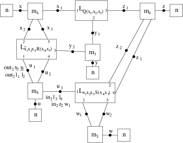
u,x,y,w,z,x_{1},y_{1},z_{1},u_{1},x_{2},y_{2},u_{2},x_{3},u_{3},z_{2},w_{1},z_{3},w_{2}\vdash\\ L_{Q(x_{1},x_{2},x_{3})}(x_{1},y_{1},z_{1})|L_{R(x_{1},x_{2})}(u_{2},x_{3})|n(u_{1})|L_{S(x_{1},x_{2})}(z_{3},w_{2})|n(u_{3})|\\ m_{4}(u,u_{1},u_{2},u_{3})|m_{4}(x,x_{1},x_{2},x_{3})|m_{3}(y,y_{1},y_{2})|m_{4}(z,z_{1},z_{2},z_{3})|m_{3}(w,w_{1},w_{2})|\\ m_{2}(x_{2},z_{2})|m_{2}(y_{2},w_{1})|n(u)|n(x)|n(y)|n(w)|n(z)

which is represented in Figure 7.

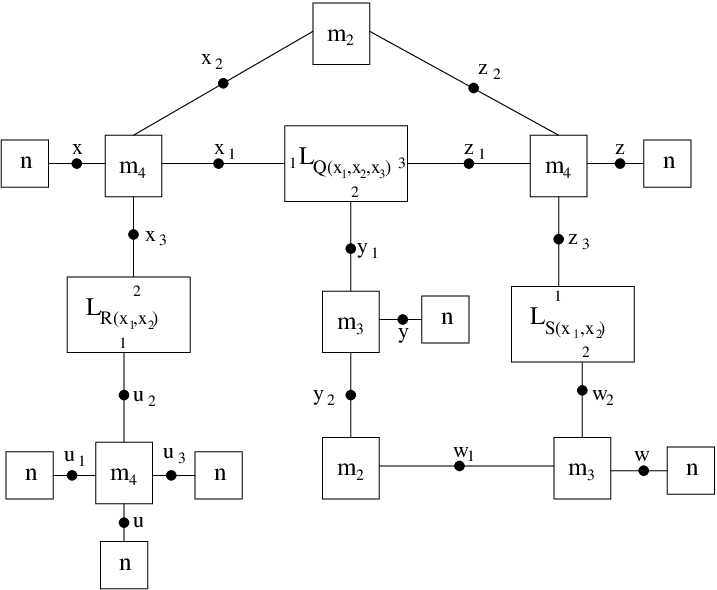
The amoeboids connect the following tuples of nodes:
$(u,u_{1},u_{2},u_{3})$ , $(x,x_{1},x_{2},x_{3},z_{2},z,z_{1},z_{3})$ , $(w,w_{1},w_{2},y_{2},y,y_{1})$ . Thus, if we connect these sets of nodes with simple amoeboids instead of with complex ones, we have up to injective renamings a translation of $(uxy)Q(x,y,x)|R(u,x)|S(x,y)$ as required.

Example 6 (Translation of a transition with recursion)

We will show here an example that uses recursion. Let us consider the closed process $(uz)\overline{u}z|\rec X.(x)ux.(\overline{u}x.0|X)$ . The translation of this process, as shown in Example 3 is:

u,z,y,u_{1},z_{1},u_{2},y_{1},u_{3},y_{2},u_{4},u_{5}\vdash\\ L_{\overline{x_{1}}x_{2}.0}(u_{1},z_{1})|L_{x_{1}x_{2}.(\overline{x_{3}}x_{4}.0|\rec X.(x)x_{5}x.(\overline{x_{6}}x.0|X))}(u_{2},y_{1},u_{3},y_{2},u_{4},u_{5})|\\ m_{6}(u,u_{1},u_{2},u_{3},u_{4},u_{5})|m_{2}(z,z_{1})|m_{3}(y,y_{1},y_{2})|n(u)|n(z)|n(y)

We need the productions for two sequential edges (for the first step): $\overline{x_{1}}x_{2}.0$ and $x_{1}x_{2}.(\overline{x_{3}}x_{4}.0|\rec X.(x)x_{5}x.(\overline{u}x_{6}.0|X))$ .
The productions are the ones of Example 4 (we write them here in a suitable $\alpha$ -converted form):

\hskip 56.9055ptu_{1},z_{1}\vdash L_{\overline{x_{1}}x_{2}.0}(u_{1},z_{1})\xrightarrow{(u_{1},out_{1},\langle z_{1}\rangle)}u_{1},z_{1}\vdash n(u_{1})\hskip 56.9055pt

u_{2},y_{1},u_{3},y_{2},u_{4},u_{5}\vdash L_{x_{1}x_{2}.(\overline{x_{3}}x_{4}.0|\rec X.(x)x_{5}x.(\overline{x_{6}}x.0|X))}(u_{2},y_{1},u_{3},y_{2},u_{4},u_{5})\\ \xrightarrow{u_{2},in_{1},\langle y_{1}\rangle}\\ u_{2},y_{1},u_{3},y_{2},u_{4},u_{5},w_{1},w_{2},w_{3},w_{4},w_{5},w_{6},y^{\prime},u^{\prime}_{4},u^{\prime}_{5}\vdash\\ L_{\overline{x_{1}}x_{2}.0}(u_{3},y_{2})|L_{x_{1}x_{2}.(\overline{x_{3}}x_{4}.0|\rec X.((x)x_{5}x.(\overline{x_{6}}x.0|X)))}(w_{1},w_{2},w_{3},w_{4},w_{5},w_{6})|\\ m_{3}(u^{\prime}_{4},w_{1},w_{5})|m_{3}(u^{\prime}_{5},w_{3},w_{6})|m_{3}(y^{\prime},w_{2},w_{4})|n(y^{\prime})|m_{2}(u_{4},u^{\prime}_{4})|m_{2}(u_{5},u^{\prime}_{5})|n(u_{2})

By using these two productions and a production for $m_{6}$ (the other edges stay idle) we have the following transition:

u,z,y,u_{1},z_{1},u_{2},y_{1},u_{3},y_{2},u_{4},u_{5}\vdash\\ L_{\overline{x_{1}}x_{2}.0}(u_{1},z_{1})|L_{x_{1}x_{2}.(\overline{x_{3}}x_{4}.0|\rec X.(x)x_{5}x.(\overline{x_{6}}x.0|X))}(u_{2},y_{1},u_{3},y_{2},u_{4},u_{5})|\\ m_{6}(u,u_{1},u_{2},u_{3},u_{4},u_{5})|m_{2}(z,z_{1})|m_{3}(y,y_{1},y_{2})|n(u)|n(z)|n(y)\\ \xrightarrow{(u_{1},out_{1},\langle z_{1}\rangle)(u_{2},in_{1},\langle y_{1}\rangle)}\\ u,y,z,x,u_{1},z_{1},u_{2},y_{1},u_{3},y_{2},u_{4},u_{5},w_{1},w_{2},w_{3},w_{4},w_{5},w_{6},y^{\prime},u^{\prime}_{4},u^{\prime}_{5}\vdash\\ n(u_{1})|L_{\overline{x_{1}}x_{2}.0}(u_{3},y_{2})|L_{x_{1}x_{2}.(\overline{x_{3}}x_{4}.0|\rec X.((x)x_{5}x.(\overline{x_{6}}x.0|X)))}(w_{1},w_{2},w_{3},w_{4},w_{5},w_{6})|\\ m_{3}(u^{\prime}_{4},w_{1},w_{5})|m_{3}(u^{\prime}_{5},w_{3},w_{6})|m_{3}(y^{\prime},w_{2},w_{4})|n(y^{\prime})|m_{2}(u_{4},u^{\prime}_{4})|m_{2}(u_{5},u^{\prime}_{5})|n(u_{2})|\\ m_{6}(u,u_{1},u_{2},u_{3},u_{4},u_{5})|m_{2}(z_{1},y_{1})|m_{2}(z,z_{1})|m_{3}(y,y_{1},y_{2})|n(u)|n(z)|n(y)

The resulting graph is, up to injective renaming and equivalence of amoeboids, a translation of:
$(uyy^{\prime})(\overline{u}y.0|uy^{\prime}.(\overline{u}y^{\prime}.0|\rec X.(x)ux.(\overline{u}x.0|X)))$
as required.

We end this section with a simple schema on the correspondence between the two models.
Fusion HSHR Fusion HSHR Closed process Graph Reduction Transition Sequential process Edge Name Amoeboid Prefix execution Production 0 $Nil$

As shown in the table, we represent (closed) processes by graphs where edges are sequential processes and amoeboids model names. The inactive process $0$ is the empty graph $nil$ . From a dynamic point of view, Fusion reductions are modelled by HSHR transitions obtained composing productions that represent prefix executions.

4 Mapping Hoare SHR into logic programming

We will now present a mapping from HSHR into a subset of logic programming called Synchronized Logic Programming (SLP). The idea is to compose this mapping with the previous one obtaining a mapping from Fusion Calculus into logic programming.

4.1 Synchronized Logic Programming

In this subsection we present Synchronized Logic Programming.
SLP has been introduced because logic programming allows for many execution strategies and for complex interactions. Essentially SLP is obtained from standard logic programming by adding a mechanism of transactions. The approach is similar to the zero-safe nets approach [1] for Petri nets. In particular we consider that function symbols are resources that can be used only inside a transaction. A transaction can thus end only when the goal contains just predicates and variables. During a transaction, which is called big-step in this setting, each atom can be rewritten at most once. If a transaction can not be terminated, then the computation is not allowed. A computation is thus a sequence of big-steps.

This synchronized flavour of logic programming corresponds to HSHR since:

•

used goals correspond to graphs (goal-graphs);
•

clauses in programs correspond to HSHR productions (synchronized clauses);
•

resulting computations model HSHR computations (synchronized computations).

Definition 18 (Goal-graph)

We call goal-graph a goal which has no function symbols (constants are considered as functions of arity $0$ ).

Definition 19 (Synchronized program)

A synchronized program is a finite set of synchronized rules, i.e. definite program clauses such that:

•

the body of each rule is a goal-graph;
•

the head of each rule is $A(t_{1},\dots,t_{n})$ where $t_{i}$ is either a variable or a single function (of arity at least $1$ ) symbol applied to variables. If it is a variable then it also appears in the body of the clause.

Example 7

$q(f(x),y)\leftarrow p(x,y)$ synchronized rule; $q(f(x),y)\leftarrow p(x,f(y))$ not synchronized since $p(x,f(y))$ is not a goal-graph; $q(g(f(x)),y)\leftarrow p(x,y)$ not synchronized since it contains nested functions; $q(f(x),y,f(z))\leftarrow p(x)$ not synchronized since $y$ is an argument of the head predicate but it does not appear in the body; $q(f(x),f(z))\leftarrow p(x)$ synchronized, even if $z$ does not appear in the body.

In the mapping, the transaction mechanism is used to model the synchronization of HSHR, where edges can be rewritten only if the synchronization constraints are satisfied. In particular, a clause $A(t_{1},\dots,t_{n})\leftarrow B_{1},\dots,B_{n}$ will represent a production where the head predicate $A$ is the label of the edge in the left hand side, and the body $B_{1},\dots,B_{n}$ is the graph in the right hand side. Term $t_{i}$ in the head represents the action occurring in $x_{i}$ , if $A(x_{1},\dots,x_{n})$ is the edge matched by the production. Intuitively, the first condition of Definition 19 says that the result of a local rewriting must be a goal-graph. The second condition forbids synchronizations with structured actions, which are not allowed in HSHR (this would correspond to allow an action in a production to synchronize with a sequence of actions from a computation of an adjacent subgraph). Furthermore it imposes that we cannot disconnect from a node without synchronizing on it ³³ 3 This condition has only the technical meaning of making impossible some rewritings in which an incorrect transition may not be forbidden because its only effect is on the discarded variable. Luckily, we can impose this condition without altering the power of the formalism, because we can always perform a special $foo$ action on the node we disconnect from and make sure that all the other edges can freely do the same action. For example we can rewrite $q(f(x),y,f(z))\leftarrow p(x)$ as $q(f(x),foo(y),f(z))\leftarrow p(x)$ , which is an allowed synchronized rule. An explicit translation of action $\epsilon$ can be used too..

Now we will define the subset of computations we are interested in.

Definition 20 (Synchronized Logic Programming)

Given a synchronized program $P$ we write:

G_{1}\stackrel{{\scriptstyle\theta}}{{\Rightarrow}}G_{2}

iff $G_{1}\xrightarrow{\theta^{\prime}}\mstar G_{2}$ and all steps performed in the computation expand different atoms of $G_{1}$ , $\theta^{\prime}|_{\n(G_{1})}=\theta$ and both $G_{1}$ and $G_{2}$ are goal-graphs.
We call $G_{1}\stackrel{{\scriptstyle\theta}}{{\Rightarrow}}G_{2}$ a big-step and all the $\rightarrow$ steps in a big-step small-steps.
A SLP computation is:
$G_{1}\Rightarrow^{*}G_{2}$ i.e. a sequence of 0 or more big-steps.

4.2 The mapping

We want to use SLP to model HSHR systems. As a first step we need to translate graphs, i.e. syntactic judgements, to goals. In this translation, edge labels are mapped into SLP predicates. Goals corresponding to graphs will have no function symbols. However function symbols will be used to represent actions. In the translation we will lose the context $\Gamma$ .

Definition 21 (Translation for syntactic judgements)

We define the translation operator $\llbracket-\rrbracket$ as:

\llbracket\Gamma\vdash L(x_{1},\dots,x_{n})\rrbracket=L(x_{1},\dots,x_{n})

\llbracket\Gamma\vdash G_{1}|G_{2}\rrbracket=\llbracket\Gamma\vdash G_{1}\rrbracket,\llbracket\Gamma\vdash G_{2}\rrbracket

\llbracket\Gamma\vdash nil\rrbracket=\square

Sometimes we will omit the $\Gamma$ part of the syntactic judgement. We can do this because it does not influence the translation. For simplicity, we suppose that the set of nodes in the SHR model coincides with the set of variables in SLP (otherwise we need a bijective translation function). We do the same for edge labels and names of predicates, and for actions and function symbols.

Definition 22

Let $\Gamma\vdash G$ and $\Gamma^{\prime}\vdash G^{\prime}$ be graphs. We define the equivalence relation $\cong$ in the following way: $\Gamma\vdash G\cong\Gamma^{\prime}\vdash G^{\prime}$ iff $G\equiv G^{\prime}$ .

Observe that if two judgements are equivalent then they can be written as:
$\Gamma,\Gamma_{unused}\vdash G$
$\Gamma,\Gamma_{unused}^{\prime}\vdash G$
where $\Gamma=\n(G)$ .

Theorem 3 (Correspondence of judgements and goal-graphs)

The operator $\llbracket-\rrbracket$ defines an isomorphism between judgements (defined up to $\cong$ ) and goal-graphs.

Proof 4.4.

The proof is straightforward observing that the operator $\llbracket-\rrbracket$ defines a bijection between representatives of syntactic judgements and representatives of goal-graphs and the congruence on the two structures is essentially the same.

We now define the translation from HSHR productions to definite clauses.

Definition 23 (Translation from productions to clauses)

We define the translation operator $\llbracket-\rrbracket$ as:

\llbracket L(x_{1},\dots,x_{n})\xrightarrow{\Lambda,\pi}G\rrbracket=L(a_{1}(x_{1}\pi,\vec{y}_{1}),\dots,a_{n}(x_{n}\pi,\vec{y}_{n}))\leftarrow\llbracket G\rrbracket

if $\Lambda(x_{i})=(a_{i},\vec{y}_{i})$ for each $i\in\{1,\dots,n\}$ and if $a_{i}\neq\epsilon$ . If $a_{i}=\epsilon$ we write simply $x_{i}\pi$ instead of $\epsilon(x_{i}\pi)$ .

The idea of the translation is that the condition given by an action $(x,a,\vec{y})$ is represented by using the term $a(x\pi,\vec{y})$ as argument in the position that corresponds to $x$ . Notice that in this term $a$ is a function symbol and $\pi$ is a substitution. During unification, $x$ will be bound to that term and, when other instances of $x$ are met, the corresponding term must contain the same function symbol (as required by Hoare synchronization) in order to be unifiable. Furthermore the corresponding tuples of transmitted nodes are unified. Since $x$ will disappear we need another variable to represent the node that corresponds to $x$ . We use the first argument of $a$ to this purpose. If two nodes are merged by $\pi$ then their successors are the same as required.

Observe that we do not need to translate all the possible variants of the rules since variants with fresh variables are automatically built when the clauses are applied. Notice also that the clauses we obtain are synchronized clauses.

The observable substitution contains information on $\Lambda$ and $\pi$ . Thus given a transition we can associate to it a substitution $\theta$ . We have different choices for $\theta$ according to where we map variables. In fact in HSHR nodes are mapped to their representatives according to $\pi$ , while, in SLP, $\theta$ cannot do the same, since the variables of the clause variant must be all fresh. The possible choices of fresh names for the variables change by an injective renaming the result of the big-step.

Definition 24 (Substitution associated to a transition)

Let $\Gamma\vdash G\xrightarrow{\Lambda,\pi}\Phi\vdash G^{\prime}$ be a transition. We say that the substitution $\theta_{\rho}$ associated to this transition is:
$\theta_{\rho}=\{(a(x\pi\rho,\vec{y}\rho)/x|\Lambda(x)=(a,\vec{y}),a\neq\epsilon\}\cup\{x\pi\rho/x\}|\Lambda(x)=(\epsilon,\langle\rangle)\}$
for some injective renaming $\rho$ .

We will now prove the correctness and the completeness of our translation.

Theorem 4.5 (Correctness).

Let $\mathcal{P}$ be a set of productions of a HSHR system as defined in definitions 9 and 10. Let $P$ be the logic program obtained by translating the productions in $\mathcal{P}$ according to Definition 23. If:
$\mathcal{P}\Vdash(\Gamma\vdash G\xrightarrow{\Lambda,\pi}\Phi\vdash G^{\prime})$
then we can have in $P$ a big-step of Synchronized Logic Programming:
$\llbracket\Gamma\vdash G\rrbracket\stackrel{{\scriptstyle\theta_{\rho}}}{{\Rightarrow}}T$
for every $\rho$ such that $x\rho$ is a fresh variable unless possibly when $x\in\Gamma\land\Lambda(x)=(\epsilon,\langle\rangle)$ . In that case we may have $x\rho=x$ . Furthermore $\theta_{\rho}$ is associated to $\Gamma\vdash G\xrightarrow{\Lambda,\pi}\Phi\vdash G^{\prime}$ and $T=\llbracket\Phi\vdash G^{\prime}\rrbracket\rho$ . Finally, used productions translate into the clauses used in the big-step and are applied to the edges that translate into the predicates rewritten by them.

Proof 4.6.

The proof is by rule induction.
See A.

Theorem 4.7 (Completeness).

Let $\mathcal{P}$ be a set of productions of a HSHR system. Let $P$ be the logic program obtained by translating the productions in $\mathcal{P}$ according to Definition 23. If we have in $P$ a big-step of logic programming:
$\llbracket\Gamma\vdash G\rrbracket\stackrel{{\scriptstyle\theta}}{{\Rightarrow}}T$
then there exist $\rho$ , $\theta^{\prime}$ , $\Lambda$ , $\pi$ , $\Phi$ and $G^{\prime}$ such that $\theta=\theta^{\prime}_{\rho}$ is associated to $\Gamma\vdash G\xrightarrow{\Lambda,\pi}\Phi\vdash G^{\prime}$ . Furthermore $T=\llbracket\Phi\vdash G^{\prime}\rrbracket\rho$ and $\mathcal{P}\Vdash(\Gamma\vdash G\xrightarrow{\Lambda,\pi}\Phi\vdash G^{\prime})$ .

Proof 4.8.

See A.

Example 8

We continue here Example 5 by showing how that fusion computation can be translated into a Synchronized Logic Programming computation.

(uxyzw)(Q(x,y,z)|\overline{u}xy.R(u,x)|uzw.S(z,w))\rightarrow\\ (uxy)(Q(x,y,z)|R(u,x)|S(z,w))\{x/z,y/w\}

Remember that a translation of the starting process is:

u,x,y,w,z,x_{1},y_{1},z_{1},u_{1},x_{2},y_{2},u_{2},x_{3},u_{3},z_{2},w_{1},z_{3},w_{2}\vdash\\ L_{Q(x_{1},x_{2},x_{3})}(x_{1},y_{1},z_{1})|L_{\overline{x_{1}}x_{2}x_{3}.R(x_{4},x_{5})}(u_{1},x_{2},y_{2},u_{2},x_{3})|\\ L_{x_{1}x_{2}x_{3}.S(x_{4},x_{5})}(u_{3},z_{2},w_{1},z_{3},w_{2})|m_{4}(u,u_{1},u_{2},u_{3})|m_{4}(x,x_{1},x_{2},x_{3})|\\ m_{3}(y,y_{1},y_{2})|m_{4}(z,z_{1},z_{2},z_{3})|m_{3}(w,w_{1},w_{2})|n(u)|n(x)|n(y)|n(w)|n(z)

We have the following productions:

y_{1},y_{2},y_{3},y_{4},y_{5}\vdash L_{\overline{x_{1}}x_{2}x_{3}.R(x_{4},x_{5})}(y_{1},y_{2},y_{3},y_{4},y_{5})\xrightarrow{(y_{1},out_{2},\langle y_{2},y_{3}\rangle)}\\ y_{1},y_{2},y_{3},y_{4},y_{5}\vdash L_{R(x_{1},x_{2})}(y_{4},y_{5})|n(y_{1})

y_{1},y_{2},y_{3},y_{4},y_{5}\vdash L_{x_{1}x_{2}x_{3}.S(x_{4},x_{5})}(y_{1},y_{2},y_{3},y_{4},y_{5})\xrightarrow{(y_{1},in_{2},\langle y_{2},y_{3}\rangle)}\\ y_{1},y_{2},y_{3},y_{4},y_{5}\vdash L_{S(x_{1},x_{2})}(y_{4},y_{5})|n(y_{1})

that corresponds to the clauses (we directly write suitably renamed variants):
$L_{\overline{x_{1}}x_{2}x_{3}.R(x_{4},x_{5})}(out_{2}(u^{\prime}_{1},x^{\prime}_{2},y^{\prime}_{2}),x^{\prime}_{2},y^{\prime}_{2},u^{\prime}_{2},x^{\prime}_{3})\leftarrow L_{R(x_{1},x_{2})}(u^{\prime}_{2},x^{\prime}_{3})|n(u^{\prime}_{1})$
$L_{x_{1}x_{2}x_{3}.S(x_{4},x_{5})}(in_{2}(u^{\prime\prime\prime}_{3},z^{\prime\prime\prime}_{2},w^{\prime\prime\prime}_{1}),z^{\prime\prime\prime}_{2},w^{\prime\prime\prime}_{1},z^{\prime\prime\prime}_{3},w^{\prime\prime\prime}_{2})\leftarrow L_{S(x_{1},x_{2})}(z^{\prime\prime\prime}_{3},w^{\prime\prime\prime}_{2})|n(u^{\prime\prime\prime}_{3})$
plus the clause obtained from the auxiliary production:

m_{4}(u^{\prime\prime},out_{2}(u^{\prime\prime}_{1},x^{\prime\prime}_{2},y^{\prime\prime}_{2}),u^{\prime\prime}_{2},in_{2}(u^{\prime\prime}_{3},z^{\prime\prime}_{2},w^{\prime\prime}_{1}))\leftarrow\\ m_{4}(u^{\prime\prime},u^{\prime\prime}_{1},u^{\prime\prime}_{2},u^{\prime\prime}_{3}),m_{2}(x^{\prime\prime}_{2},z^{\prime\prime}_{2}),m_{2}(y^{\prime\prime}_{2},w^{\prime\prime}_{1})

We obtain the big-step represented in Figure 8.

Figure 8: Big-step for a Fusion transition

L_{Q(x_{1},x_{2},x_{3})}(x_{1},y_{1},z_{1}),L_{\overline{x_{1}}x_{2}x_{3}.R(x_{4},x_{5})}(u_{1},x_{2},y_{2},u_{2},x_{3}),\\ L_{x_{1}x_{2}x_{3}.S(x_{4},x_{5})}(u_{3},z_{2},w_{1},z_{3},w_{2}),\\ m_{4}(u,u_{1},u_{2},u_{3}),m_{4}(x,x_{1},x_{2},x_{3}),m_{3}(y,y_{1},y_{2}),m_{4}(z,z_{1},z_{2},z_{3}),m_{3}(w,w_{1},w_{2}),\\ n(u),n(x),n(y),n(w),n(z)\\ \xrightarrow{out_{2}(u^{\prime}_{1},x_{2},y_{2})/u_{1},x_{2}/x^{\prime}_{2},y_{2}/y^{\prime}_{2},u_{2}/u^{\prime}_{2},x_{3}/x^{\prime}_{3}}\\ L_{Q(x_{1},x_{2},x_{3})}(x_{1},y_{1},z_{1}),L_{R(x_{1},x_{2})}(u_{2},x_{3}),n(u^{\prime}_{1}),L_{x_{1}x_{2}x_{3}.S(x_{4},x_{5})}(u_{3},z_{2},w_{1},z_{3},w_{2}),\\ m_{4}(u,out_{2}(u^{\prime}_{1},x_{2},y_{2}),u_{2},u_{3}),m_{4}(x,x_{1},x_{2},x_{3}),m_{3}(y,y_{1},y_{2}),\\ m_{4}(z,z_{1},z_{2},z_{3}),m_{3}(w,w_{1},w_{2}),n(u),n(x),n(y),n(w),n(z)\\ \xrightarrow{u/u^{\prime\prime},u^{\prime}_{1}/u^{\prime\prime}_{1},x_{2}/x^{\prime\prime}_{2},y_{2}/y^{\prime\prime}_{2},u_{2}/u^{\prime\prime}_{2},in_{2}(u^{\prime\prime}_{3},z^{\prime\prime}_{2},w^{\prime\prime}_{1})/u_{3}}\\ L_{Q(x_{1},x_{2},x_{3})}(x_{1},y_{1},z_{1}),L_{R(x_{1},x_{2})}(u_{2},x_{3}),n(u^{\prime}_{1}),\\ L_{x_{1}x_{2}x_{3}.S(x_{4},x_{5})}(in_{2}(u^{\prime\prime}_{3},z^{\prime\prime}_{2},w^{\prime\prime}_{1}),z_{2},w_{1},z_{3},w_{2}),\\ m_{4}(u,u^{\prime}_{1},u_{2},u^{\prime\prime}_{3}),m_{2}(x_{2},z^{\prime\prime}_{2}),m_{2}(y_{2},w^{\prime\prime}_{1}),m_{4}(x,x_{1},x_{2},x_{3}),m_{3}(y,y_{1},y_{2}),\\ m_{4}(z,z_{1},z_{2},z_{3}),m_{3}(w,w_{1},w_{2}),n(u),n(x),n(y),n(w),n(z)\\ \xrightarrow{u^{\prime\prime}_{3}/u^{\prime\prime\prime}_{3},z_{2}/z^{\prime\prime}_{2},w_{1}/w^{\prime\prime}_{1},z_{2}/z^{\prime\prime\prime}_{2},w_{1}/w^{\prime\prime\prime}_{1},z_{3}/z^{\prime\prime\prime}_{3},w_{2}/w^{\prime\prime\prime}_{2}}\\ L_{Q(x_{1},x_{2},x_{3})}(x_{1},y_{1},z_{1}),L_{R(x_{1},x_{2})}(u_{2},x_{3}),n(u^{\prime}_{1}),L_{S(x_{1},x_{2})}(z_{3},w_{2}),n(u^{\prime\prime}_{3}),\\ m_{4}(u,u^{\prime}_{1},u_{2},u^{\prime\prime}_{3}),m_{2}(x_{2},z_{2}),m_{2}(y_{2},w_{1}),m_{4}(x,x_{1},x_{2},x_{3}),m_{3}(y,y_{1},y_{2}),\\ m_{4}(z,z_{1},z_{2},z_{3}),m_{3}(w,w_{1},w_{2}),n(u),n(x),n(y),n(w),n(z)

The observable substitution of the big-step is $\{out_{2}(u^{\prime}_{1},x_{2},y_{2})/u_{1},in_{2}(u^{\prime\prime}_{3},z_{2},w_{1})/u_{3}\}$ . This is associated to the wanted HSHR transition with $\rho=\{u^{\prime}_{1}/u_{1},u^{\prime\prime}_{3}/u_{3}\}$ and by applying $\rho$ to the final graph of the HSHR transition we obtain:

L_{Q(x_{1},x_{2},x_{3})}(x_{1},y_{1},z_{1})|L_{R(x_{1},x_{2})}(u_{2},x_{3})|n(u^{\prime}_{1})|L_{S(x_{1},x_{2})}(z_{3},w_{2})|n(u^{\prime\prime}_{3})|\\ m_{4}(u,u^{\prime}_{1},u_{2},u^{\prime\prime}_{3})|m_{4}(x,x_{1},x_{2},x_{3})|m_{3}(y,y_{1},y_{2})|m_{4}(z,z_{1},z_{2},z_{3})|m_{3}(w,w_{1},w_{2})|\\ m_{2}(x_{2},z_{2})|m_{2}(y_{2},w_{1})|n(u)|n(x)|n(y)|n(w)|n(z)

that, translated, becomes the final goal of the big-step as required.

We end this section with a simple schema on the correspondence between the two models.
HSHR SLP HSHR SLP Graph Goal Transition Big-step Edge Atomic goal Node Variable Parallel comp. And comp. $Nil$ $\square$ Production Clause Action Function s.

Essentially the correspondence is given by the homomorphism between graphs and goals, with edges mapped to atomic goals, nodes to variables, parallel composition to And composition and $nil$ to $\square$ . Dynamically, HSHR transitions are modelled by big-steps, that are transactional applications of clauses which model productions. Finally, HSHR actions are modelled by function symbols.

4.3 Using Prolog to implement Fusion Calculus

The theorems seen in the previous sections can be used for implementation purposes. As far as Synchronized Logic Programming is concerned, in [14] (?) a simple meta-interpreter is presented.

The idea is to use Prolog ability of dynamically changing the clause database to insert into it a set of clauses and a goal and to compute the possible synchronized computations of given length. This can be directly used to simulate HSHR transitions. In order to simulate Fusion Calculus processes we have to implement amoeboids using a bounded number of different connectors (note that $m_{2}$ , $m_{3}$ and $n$ are enough) and to implement in the meta-interpreter the condition under which productions can be applied in a single big-step. This can be easily done. Furthermore this decreases the possible choices of applicable productions and thus improves the efficiency w.r.t. the general case.

5 Conclusion

In this paper we have analyzed the relationships between three different formalisms, namely Fusion Calculus, HSHR and logic programming.

The correspondence between HSHR and the chosen transactional version of logic programming, SLP, is complete and quite natural. Thus we can consider HSHR as a “subcalculus” of (synchronized) logic programming.

The mapping between Fusion Calculus and HSHR is instead more involved because it has to deal with many important differences:

•

process calculi features vs graph transformation features;
•

interleaving models vs concurrent models;
•

Milner synchronization vs Hoare synchronization.

Hoare synchronization was necessary since our aim was to eventually map Fusion Calculus to logic programming. If the aim is just to compare Fusion Calculus and SHR it is possible to use SHR with Milner synchronization, achieving a much simpler and complete mapping, which considers the LTS of Fusion Calculus instead of reductions (see [17]).

We think that the present work can suggest several interesting lines of development, dictated by the comparison of the three formalisms studied in the paper. First, our implementation of routers in terms of amoeboids is rather general and abstract, and shows that Fusion Calculus names are a rather high level concept. They abstract out the behaviour of an underlying network of connections which must be open and reconfigurable. Had we chosen $\pi$ -calculus instead (see a translation of $\pi$ -calculus to Milner SHR in [11]), we would have noticed important differences. For instance, fusions are also considered in the semantics of open $\pi$ -calculus by Davide Sangiorgi [23], but in that work not all the names can be fused: newly extruded names cannot be merged with previously generated names. This is essential for specifying nonces and session keys for secure protocols. Instead, Fusion Calculus does not provide equivalent constructs. Looking at our translation, we can conclude that logic programming does not offer this feature, either. Thus logic programming is a suitable counterpart of Fusion Calculus, but it should be properly extended for matching open $\pi$ -calculus and security applications.

In a similar line of thought, we observe that we have a scope restriction operator in the Fusion Calculus, but no restriction is found in our version of HSHR. We think this omission simplifies our development, since no restriction exists in ordinary logic programming, either. However versions of SHR with restriction have been considered [11, 6, 14]. Also (synchronized) logic programming can be smoothly extended with a restriction operator [14]. More importantly, Fusion Calculus is equipped with an observational abstract semantics based on (hyper) bisimulation. We did not consider a similar concept for SHR or logic programming, since we considered it outside the scope of the paper. Furthermore our operational correspondence between HSHR and SLP is very strong and it should respect any reasonable abstract semantics. The mapping from Fusion Calculus into HSHR deals only with closed terms, thus no observations can be considered. However a bisimulation semantics of SHR has been considered in [13], and an observational semantics of logic programming is discussed in [2].

Another comment concerns concurrency. To prove the equivalence of Fusion Calculus and of its translation into HSHR we had to restrict the possible computations of the latter. On the contrary, if all computations were allowed, the same translation would yield a concurrent semantics of Fusion Calculus, that we think is worth studying. For instance in the presence of concurrent computations not all equivalent amoeboids would have the same behaviour, since some of them would allow for more parallelism than others.

Finally we would like to emphasize some practical implication of our work. In fact, logic programming is not only a model of computation, but also a well developed programming paradigm. Following the lines of our translation, implementations of languages based on Fusion Calculus and HSHR could be designed, allowing to exploit existing ideas, algorithms and tools developed for logic programming.

References

Bruni and Montanari (2000) Bruni, R. and Montanari, U. 2000. Zero-safe nets: Comparing the collective and individual token approaches. Information and Computation 156, 1-2, 46–89.
Bruni et al. (2001) Bruni, R., Montanari, U., and Rossi, F. 2001. An interactive semantics of logic programming. Theory and Practice of Logic Programming 1, 6, 647–690.
Degano and Montanari (1987) Degano, P. and Montanari, U. 1987. A model for distributed systems based on graph rewriting. Journal of the ACM (JACM) 34, 2, 411–449.
Ehrig et al. (1999) Ehrig, H., Kreowski, H.-J., Montanari, U., and Rozenberg, G., Eds. 1999. Handbook of Graph Grammars and Computing by Graph Transformation, Vol.3: Concurrency, Parallelism, and Distribution. World Scientific.
Ehrig et al. (1973) Ehrig, H., Pfender, M., and Schneider, H. J. 1973. Graph grammars: an algebraic approach. In Proc. of IEEE Conference on Automata and Switching Theory. IEEE Computer Society, 167–180.
Ferrari et al. (2001) Ferrari, G. L., Montanari, U., and Tuosto, E. 2001. A LTS semantics of ambients via graph synchronization with mobility. In Proc. of ICTCS’01. LNCS, vol. 2202. Springer, 1–16.
Gardner and Wischik (2000) Gardner, P. and Wischik, L. 2000. Explicit fusions. In Mathematical Foundations of Computer Science. 373–382.
Gardner and Wischik (2004) Gardner, P. and Wischik, L. 2004. Strong bisimulation for the explicit fusion calculus. In Proc. of FoSSaCS’04. LNCS, vol. 2987. Springer, 484–498.
Hirsch (2003) Hirsch, D. 2003. Graph transformation models for software architecture styles. Ph.D. thesis, Departamento de Computación, Facultad de Ciencias Exactas y Naturales, Universidad de Buenos Aires, Argentina.
Hirsch et al. (2000) Hirsch, D., Inverardi, P., and Montanari, U. 2000. Reconfiguration of software architecture styles with name mobility. In Proc. of COORDINATION 2000. LNCS, vol. 1906. Springer, 148–163.
Hirsch and Montanari (2001) Hirsch, D. and Montanari, U. 2001. Synchronized hyperedge replacement with name mobility. In Proc. of CONCUR’01. LNCS, vol. 2154. Springer, 121–136.
Jensen and Milner (2003) Jensen, O. H. and Milner, R. 2003. Bigraphs and transitions. SIGPLAN Not. 38, 1, 38–49.
König and Montanari (2001) König, B. and Montanari, U. 2001. Observational equivalence for synchronized graph rewriting. In Proc. of TACS’01. LNCS, vol. 2215. Springer, 145–164.
Lanese (2002) Lanese, I. 2002. Process synchronization in distributed systems via Horn clauses. M.S. thesis, Computer Science Department, University of Pisa, Pisa, Italy. Downloadable from http://www.di.unipi.it/˜lanese/tesi.ps.
Lanese (2006) Lanese, I. 2006. Synchronization strategies for global computing models. Ph.D. thesis, Computer Science Department, University of Pisa, Pisa, Italy. Forthcoming.
Lanese and Montanari (2002) Lanese, I. and Montanari, U. 2002. Software architectures, global computing and graph transformation via logic programming. In Proc SBES’2002 - 16th Brazilian Symposium on Software Engineering. Anais, 11–35.
Lanese and Montanari (2004a) Lanese, I. and Montanari, U. 2004a. A graphical fusion calculus. In Proc. of the Workshop of the COMETA Project on Computational Metamodels. Electronic Notes in Theoretical Computer Science, vol. 104. Elsevier Science, 199–215.
Lanese and Montanari (2004b) Lanese, I. and Montanari, U. 2004b. Synchronization algebras with mobility for graph transformations. In Proc. of FGUC’04 – Foundations of Global Ubiquitous Computing. Electronic Notes in Theoretical Computer Science, vol. 138. Elsevier Science, 43–60.
Lloyd (1993) Lloyd, J. W. 1993. Foundations of Logic Programming, Second Extended Edition. Springer.
Milner et al. (1992) Milner, R., Parrow, J., and Walker, D. 1992. A calculus of mobile processes. Information and Computation 100, 1–77.
Palamidessi (1990) Palamidessi, C. 1990. Algebraic properties of idempotent substitutions. In Proc. of ICALP’90. LNCS, vol. 443. Springer, 386–399.
Parrow and Victor (1998) Parrow, J. and Victor, B. 1998. The fusion calculus: Expressiveness and symmetry in mobile processes. In Proc. of LICS ’98. IEEE, Computer Society Press.
Sangiorgi (1993) Sangiorgi, D. 1993. A theory of bisimulation for the pi-calculus. In Proc. of CONCUR’93. LNCS, vol. 715. Springer, 127–142.
Victor (1998) Victor, B. 1998. The fusion calculus: Expressiveness and symmetry in mobile processes. Ph.D. thesis, Dept. of Computer Systems, Uppsala University, Sweden.

Appendix A Proofs

We have here the proofs that are missing in the main part and some lemmas used in these proofs. Lemmas are just before the proofs that use them.

Proof A.9 (Proof of Lemma 2).

Notice that all the auxiliary productions perform two non trivial actions, and because of Hoare synchronization and because each node is shared by at most two edges, synchronizing edges form chains. There are two alternatives: each chain either starts and begins on an external node, or it is a cycle that contains only internal nodes. Exactly one chain must be of the first type. In fact if we have no chain of that kind we have only trivial actions on nodes in $S$ . Also, if we have more than one, we have more than two non trivial actions on nodes in $S$ . Thanks to the last condition of Definition 17 this chain contains an odd number of connectors, which must be $m$ connectors. One can easily check by induction on the (odd) length of the chain that the transition creates an amoeboid $M(\vec{y}_{1}[i],\vec{y}_{2}[i])$ for each component of vectors $\vec{y}_{1}$ and $\vec{y}_{2}$ of fresh names and that these vectors are exposed on the external nodes together with an $in_{n}$ and an $out_{n}$ action, where $n=|\vec{y}_{1}|=|\vec{y}_{2}|$ .

Let us now consider the other kind of chains: these chains produce rings of $m_{2}$ edges connected only to fresh nodes, which thus correspond to isolate subgraphs. Furthermore, they affect only the labels of internal nodes as required.

Lemma A.10.

Given a set of amoeboids for $\sigma$ and a substitutive effect $\theta$ of a fusion $\phi=\{x_{i}=y_{i}|i=1\dots n\}$ then $\llbracket\sigma\rrbracket|\bigpar_{i=1\dots n}M(x_{i},y_{i})$ is a set of amoeboids for $\sigma\theta$ .

Proof A.11.

Since we are working up to injective renamings we only have to prove that two names are connected by $\llbracket\sigma\rrbracket|\bigpar_{i=1\dots n}M(x_{i},y_{i})$ iff they are merged by $\sigma\theta$ and that all the paths connecting external nodes in the final graph have odd length. By definition two names are connected by $\llbracket\sigma\rrbracket$ iff they are merged by $\sigma$ . Assume that two names $x$ and $y$ are merged by $\sigma\theta$ . Then their images along $\sigma$ are merged by $\theta$ . This means that we have in $\phi$ a chain of equalities from $x\sigma$ to $y\sigma$ . Thus we have amoeboids connecting the amoeboids of $x\sigma$ and of $y\sigma$ , thus $x$ and $y$ are connected. Assume now that $x$ and $y$ are connected. Then there exists an amoeboid connecting the amoeboids for $x\sigma$ and for $y\sigma$ . Thus $\theta$ merges $x\sigma$ and $y\sigma$ as required. Finally note that all the paths between external nodes are created by connecting existing paths via new amoeboids. In particular, each new path is composed by $n$ old paths and $n-1$ new amoeboids. Thus its length is the sum of $2n-1$ odd lengths and thus it is odd.

Proof A.12 (Proof of Theorem 1).

The proof is by rule induction on the reduction semantics.
Let us consider the reduction rule:

(\vec{z})(R|(\dots+u\vec{x}.P)|(\overline{u}\vec{y}.Q+\dots))\rightarrow(\vec{z})(R|P|Q)\sigma

where $|\vec{x}|=|\vec{y}|$ and $\sigma$ is a substitutive effect of $\{\vec{x}=\vec{y}\}$ such that $\dom(\sigma)\subseteq\vec{z}$ .

In order for that process to be in the standard form we just need to make $R$ sequential by unfolding recursion and taking bound names to the outside if required. For simplicity, we show just the case where $R$ is already sequential, the other being essentially equal.

Let $P_{1}$ be $(\dots+u\vec{x}.P)$ and $Q_{1}$ be $(\overline{u}\vec{y}.Q+\dots)$ .

The translation of the LHS has the form:

\Gamma\vdash L_{\hat{R}^{\prime}}(\vec{r})|L_{\hat{P}^{\prime}_{1}}(\vec{p}_{1})|L_{\hat{Q}^{\prime}_{1}}(\vec{q}_{1})|\llbracket\theta\rrbracket|\bigpar_{x\in\vec{v}}n(x)

where $R^{\prime}=\hat{R}^{\prime}\rho_{R^{\prime}}$ , $P^{\prime}_{1}=\hat{P}^{\prime}_{1}\rho_{P^{\prime}_{1}}$ , $Q^{\prime}_{1}=\hat{Q}^{\prime}_{1}\rho_{Q^{\prime}_{1}}$ and $R^{\prime}\theta=R$ , $P^{\prime}_{1}\theta=P_{1}$ , $Q^{\prime}_{1}\theta=Q_{1}$ . We also use $(u^{\prime}_{1}\vec{x}^{\prime}.P^{\prime})\theta=u\vec{x}.P$ and $(u^{\prime}_{2}\vec{y}^{\prime}.Q^{\prime})\theta=u\vec{y}.Q$ .

We have for $L_{\hat{P}^{\prime}_{1}}$ and $L_{\hat{Q}^{\prime}_{1}}$ the two following productions:

\vec{p}_{1}\vdash L_{\hat{P}^{\prime}_{1}}(\vec{p}_{1})\xrightarrow{(u^{\prime}_{1},in_{|\vec{x}^{\prime}|},\vec{x}^{\prime})}\vec{p}_{1},\vec{x}^{\prime},\vec{v}_{P}\vdash\llbracket P\rrbracket_{\vec{v}_{p},\vec{w}_{P}}|\bigpar_{x\in\Gamma^{\prime\prime}_{P}}n(x)

\vec{q}_{1}\vdash L_{\hat{Q}^{\prime}_{1}}(\vec{q}_{1})\xrightarrow{(u^{\prime}_{2},out_{|\vec{y}^{\prime}|},\vec{y}^{\prime})}\vec{q}_{1},\vec{y}^{\prime},\vec{v}_{Q}\vdash\llbracket Q\rrbracket_{\vec{v}_{Q},\vec{w}_{Q}}|\bigpar_{x\in\Gamma^{\prime\prime}_{Q}}n(x)

The choice of the parameters $\vec{v}_{P}$ and $\vec{v}_{Q}$ is not important since they are fresh names and we work up to injective renamings. The choice of $\vec{w}_{P}$ and $\vec{w}_{Q}$ is important instead, since they have to correspond to the nodes in the LHS that are still used by the process. The choice performed in Definition 15 ensures that.

Note that $\llbracket\theta\rrbracket$ contains an amoeboid for a set $U$ with $u^{\prime}_{1},u^{\prime}_{2}\in U$ . Thus from Lemma 2 the two above productions can synchronize via the amoeboid. Using rule (idle) for the other edges, we obtain as a result:

\Gamma,\Gamma_{Int}\vdash L_{\hat{R}^{\prime}}(\vec{r})|\llbracket P\rrbracket_{\vec{v}_{P},\vec{w}_{P}}|\bigpar_{x\in\Gamma^{\prime\prime}_{P}}n(x)|\llbracket Q\rrbracket_{\vec{v}_{Q},\vec{w}_{Q}}|\bigpar_{x\in\Gamma^{\prime\prime}_{Q}}n(x)|\llbracket\theta\rrbracket|\bigpar_{x\in\vec{v}}n(x)|\\ \bigpar_{i=1\dots|\vec{x}^{\prime}|}M(\vec{x}^{\prime}[i],\vec{y}^{\prime}[i])|\bigpar\tilde{M}(\emptyset)

Note that the fusion $\pi$ of the transition is the identity since each synchronization involves two edges, and at least one of them is an amoeboid which exposes fresh names. Furthermore amoeboids expose each fresh name twice. Thus no names in $\Gamma$ are merged.

Also, in the final graph each node is shared by two edges. In fact, the only connections whose cardinality is not preserved by productions are the ones between nodes whose references are exposed, namely $\vec{x}^{\prime}$ and $\vec{y}^{\prime}$ , and the corresponding process edges, but these nodes are connected to the new $M$ amoeboids created by the auxiliary productions.

In particular, $\bigpar_{x\in\Gamma^{\prime\prime}_{P}}n(x)|\bigpar_{x\in\Gamma^{\prime\prime}_{Q}}n(x)|\llbracket\theta\rrbracket$ is an amoeboid for $\theta|_{\fn(R^{\prime}|P^{\prime}|Q^{\prime})}$ . Furthermore thanks to Lemma A.10 by adding in parallel $\bigpar_{i=1\dots|\vec{x}^{\prime}|}M(\vec{x}^{\prime}[i],\vec{y}^{\prime}[i])$ we obtain an amoeboid for $\theta|_{\fn(R^{\prime}|P^{\prime}|Q^{\prime})}\sigma$ .

Thus we can rewrite the final graph up to pseudoamoeboids as:

\Gamma,\Gamma_{Int}\vdash L_{\hat{R}^{\prime}}(\vec{r})|\llbracket P\rrbracket_{\vec{v}_{P},\vec{w}_{P}}|\llbracket Q\rrbracket_{\vec{v}_{Q},\vec{w}_{Q}}|\llbracket\theta|_{\fn(R^{\prime}|P^{\prime}|Q^{\prime})}\sigma\rrbracket|\bigpar_{x\in\vec{v}}n(x)

The RHS of the fusion rule is $(\vec{z})(R|P|Q)\sigma$ , which has to be normalized into $(\vec{z}\vec{v}_{P}\vec{v}_{Q})(R|\tilde{P}|\tilde{Q})\theta_{1}\sigma$ with $(\vec{v}_{P})\tilde{P}\equiv P$ and $(\vec{v}_{Q})\tilde{Q}\equiv Q$ . Furthermore we can choose the names (since we are reasoning up to injective renamings) in such a way that $\theta_{1}=\theta|_{\fn(R^{\prime}|P^{\prime}|Q^{\prime})}$ (plus an injective renaming on names in $\vec{v}_{p}$ and $\vec{v}_{Q}$ which corresponds to an equivalence on the resulting amoeboids).

Thus the translation of the RHS is equivalent to:

\Gamma,\Gamma_{Int^{\prime}}\vdash L_{\hat{R}^{\prime}}(\vec{r})|\llbracket P\rrbracket_{\vec{v}_{P},\vec{w}_{P}}|\llbracket Q\rrbracket_{\vec{v}_{Q},\vec{w}_{Q}}|\llbracket\theta_{1}\sigma\rrbracket|\bigpar_{x\in\vec{v}}n(x)

The correctness of the rule follows.

Let us consider now rule:

(\vec{z})(R|(\dots+\phi.P))\rightarrow(\vec{z})(R|P)\sigma

where $\sigma$ is a substitutive effect of $\phi$ such that $\dom(\sigma)\subseteq\vec{z}$ .

We use essentially the same technique as before. Let us suppose $R$ already sequential. Let $P_{1}$ be $\dots+\phi.P$ . The translation of the LHS has the form:

\Gamma\vdash L_{\hat{R}^{\prime}}(\vec{r})|L_{\hat{P}^{\prime}_{1}}(\vec{p}_{1})|\llbracket\theta\rrbracket|\bigpar_{x\in\vec{v}}n(x)

where $R^{\prime}=\hat{R}^{\prime}\rho_{R^{\prime}}$ , $P^{\prime}_{1}=\hat{P}^{\prime}_{1}\rho_{P^{\prime}_{1}}$ and $R^{\prime}\theta=R$ , $P^{\prime}_{1}\theta=P_{1}$ . We also use $(\phi^{\prime}.P^{\prime})\theta=\phi.P$ .

We have for $L_{\hat{P}^{\prime}_{1}}$ the following production:

\vec{p}_{1}\vdash L_{\hat{P}^{\prime}_{1}}(\vec{p}_{1})\xrightarrow{\Lambda_{\epsilon}}\vec{p}_{1},\vec{v}_{P}\vdash\llbracket P\rrbracket_{\vec{v}_{P},\vec{w}_{P}}|\llbracket\sigma\rrbracket|\bigpar_{x\in\Gamma^{\prime\prime}}n(x)

For $\vec{v}_{P}$ and $\vec{w}_{P}$ the considerations for the preceding rule are still valid.

Using rule (idle) for the other edges, we obtain as a result:

\Gamma,\Gamma_{Int}\vdash L_{\hat{R}^{\prime}}(\vec{r})|\llbracket P\rrbracket_{\vec{v}_{P},\vec{w}_{P}}|\llbracket\sigma\rrbracket|\bigpar_{x\in\Gamma^{\prime\prime}_{P}}n(x)|\llbracket\theta\rrbracket|\bigpar_{x\in\vec{v}}n(x)

Note that the fusion part of the transition label is an identity since we have only trivial synchronizations.

Also, in the final graph each node is shared by two edges since the production preserves the cardinality of connected edges for each node.

In particular, $\bigpar_{x\in\Gamma^{\prime\prime}_{P}}n(x)|\llbracket\theta\rrbracket$ is an amoeboid for $\theta|_{\fn(R^{\prime}|P^{\prime})}$ . Furthermore, note that $\llbracket\sigma\rrbracket$ has the form $\bigpar_{i=1\dots n}m_{2}(x_{i},y_{i})$ and thus thanks to Lemma A.10 by adding it in parallel we obtain an amoeboid for $\theta|_{\fn(R^{\prime}|P^{\prime})}\sigma$ .

Thus we can rewrite the final graph as:

\Gamma,\Gamma_{Int}\vdash L_{\hat{R}^{\prime}}(\vec{r})|\llbracket P\rrbracket_{\vec{v}_{P},\vec{w}_{P}}|\llbracket\theta|_{\fn(R^{\prime}|P^{\prime})}\sigma\rrbracket|\bigpar_{x\in\vec{v}}n(x)

The RHS of the fusion rule is $(\vec{z})(R|P)\sigma$ , which has to be normalized into $(\vec{z}\vec{v}_{P})(R|\tilde{P})\theta_{1}\sigma$ with $(\vec{v}_{P})\tilde{P}\equiv P$ . Furthermore we can choose the names (since we are reasoning up to injective renamings) in such a way that $\theta_{1}=\theta|_{\fn(R^{\prime}|P^{\prime})}$ (plus an injective renaming on names in $\vec{v}_{P}$ which corresponds to an equivalence on the resulting amoeboids).

Thus the translation of the RHS is equivalent to:

\Gamma,\Gamma_{Int^{\prime}}\vdash L_{\hat{R}^{\prime}}(\vec{r})|\llbracket P\rrbracket_{\vec{v}_{P},\vec{w}_{P}}|\llbracket\theta_{1}\sigma\rrbracket|\bigpar_{x\in\vec{v}}n(x)

The correctness of the rule follows.

Consider now the rule:

\frac{P\equiv P^{\prime},P^{\prime}\rightarrow Q^{\prime},Q^{\prime}\equiv Q}{P\rightarrow Q}

Equivalent agents are converted into the same representative (up to $\alpha$ -conversion) before being translated, thus the translation of $P$ and $P^{\prime}$ are equal up to injective renamings. Similarly for the translation of $Q$ and $Q^{\prime}$ , thus the thesis follows.

Lemma A.13.

Let $\theta_{1}$ and $\theta_{2}$ be idempotent substitutions. Let $\eqn(\theta_{1})=\{x=y|x/y\in\theta_{1}\}$ . Then $\mgu(\eqn(\theta_{1})\cup\eqn(\theta_{2}))=\theta_{1}\mgu(\eqn(\theta_{2})\theta_{1})$ .

Proof A.14.

See ?).

Lemma A.15.

Given a graph $\Gamma\vdash G$ and one or zero productions for each edge in $G$ let:
$\Gamma\vdash G\xrightarrow{\Lambda_{1},\pi_{1}}\Phi_{1}\vdash G^{\prime}_{1}$
$\Gamma\vdash G\xrightarrow{\Lambda_{2},\pi_{2}}\Phi_{2}\vdash G^{\prime}_{2}$
be two transitions obtained by applying the chosen production for each edge (and using the (idle) rule if no production is chosen). Then there exists an injective renaming $\sigma$ such that:

•

$\Lambda_{1}(x)=\sigma(\Lambda_{2}(x))$ if $x$ is not an isolated node;
•

$\pi_{1}=\sigma\pi_{2}$ ;
•

$\Phi_{1}=\sigma(\Phi_{2})$ ;
•

$G^{\prime}_{1}=\sigma(G^{\prime}_{2})$ .

Proof A.16.

The proof is a simple rule induction if one proves that derivations can be done in a standard way, namely by applying to the axioms first rules (par), then rule (merge) and finally rules (new). This can be proved by showing that one can exchange the order of rules and that one can substitute two applications of (merge) with substitutions $\sigma$ and $\sigma^{\prime}$ with just one application with substitution $\sigma^{\prime}\sigma$ . We have many cases to consider, but they are not so interesting. As examples we will show the detailed proof for commutation of rule (merge) and (par) and for composition of two different rules (merge).

Let us consider the first case. Suppose we have a part of a derivation of the form:

\Gamma\sigma,\Gamma^{\prime}\vdash G_{1}\sigma|G^{\prime}_{1}\xrightarrow{\Lambda_{1}\cup\Lambda^{\prime},\pi_{1}\cup\pi^{\prime}}\Phi_{1},\Phi^{\prime}\vdash G_{2}\sigma\rho|G^{\prime}_{2}\lx@proof@logical@and\Gamma\sigma\vdash G_{1}\sigma\xrightarrow{\Lambda_{1},\pi_{1}}\Phi_{1}\vdash G_{2}\sigma\rho\Gamma\vdash G_{1}\xrightarrow{\Lambda,\pi}\Phi\vdash G_{2}\Gamma^{\prime}\vdash G^{\prime}_{1}\xrightarrow{\Lambda^{\prime},\pi^{\prime}}\Phi^{\prime}\vdash G^{\prime}_{2}

(1)

where for readability we have not written explicitly the side conditions (see Definition 10). Then we must also have a derivation for the same transition obtained applying rule (par) first and then rule (merge):

(\Gamma,\Gamma^{\prime})\sigma\vdash(G_{1}|G^{\prime}_{1})\sigma\xrightarrow{\Lambda^{\prime\prime},\pi^{\prime\prime}}\Phi^{\prime\prime}\vdash(G_{2}|G^{\prime}_{2})\sigma\rho^{\prime}\Gamma,\Gamma^{\prime}\vdash G_{1}|G^{\prime}_{1}\xrightarrow{\Lambda\cup\Lambda^{\prime},\pi\cup\pi^{\prime}}\Phi,\Phi^{\prime}\vdash G_{2}|G^{\prime}_{2}\lx@proof@logical@and\Gamma\vdash G_{1}\xrightarrow{\Lambda,\pi}\Phi\vdash G_{2}\Gamma^{\prime}\vdash G^{\prime}_{1}\xrightarrow{\Lambda^{\prime},\pi^{\prime}}\Phi^{\prime}\vdash G^{\prime}_{2}

(2)

We have to prove that this derivation is allowed and that the resulting transition is the one derived also by derivation 1. The first step is allowed iff $(\Gamma\cup\Phi)\cap(\Gamma^{\prime}\cup\Phi^{\prime})=\emptyset$ . Since the first derivation is allowed by hypothesis, then $(\Gamma\sigma\cup\Phi_{1})\cap(\Gamma^{\prime}\cup\Phi^{\prime})=\emptyset$ . Thus the only problem is when a name which is after renamed (by $\sigma$ or $\rho$ ) creates a conflict. In that case thanks to Lemma 1 we can suppose to start with a different name. The final result of the derivation is not changed by that since the name disappears. Thus the first step is legal.

For the second step we need $\forall x,y\in\Gamma,\Gamma^{\prime}.x\sigma=y\sigma\wedge x\neq y\Rightarrow\act_{\Lambda\cup\Lambda^{\prime}}(x)=\act_{\Lambda\cup\Lambda^{\prime}}(y)$ . Note that since $(\Gamma\cup\Phi)\cap(\Gamma^{\prime}\cup\Phi^{\prime})=\emptyset$ and $\sigma:\Gamma\rightarrow\Gamma$ , we have that $\sigma$ is the identity on $\Gamma^{\prime}$ , thus the only $x,y$ such that $x\sigma=y\sigma\wedge x\neq y$ are in $\Gamma$ , thus the condition is satisfied since it was satisfied in derivation 1. Furthermore we have $(\Gamma,\Gamma^{\prime})\sigma=\Gamma\sigma,\Gamma^{\prime}$ and $(G_{1}|G^{\prime}_{1})\sigma=G_{1}\sigma|G^{\prime}_{1}$ .

We must now consider $\rho^{\prime}$ . We have:

\rho^{\prime}=\mgu(\{(\n_{\Lambda\cup\Lambda^{\prime}}(x))\sigma=(\n_{\Lambda\cup\Lambda^{\prime}}(y))\sigma|x\sigma=y\sigma\}\cup\{x\sigma=y\sigma|x(\pi\cup\pi^{\prime})=y(\pi\cup\pi^{\prime})\})

For what already said we have $\rho^{\prime}=\mgu(\{(\n_{\Lambda}(x))\sigma=(\n_{\Lambda}(y))\sigma|x\sigma=y\sigma\}\cup\{x\sigma=y\sigma|x\pi=y\pi\}\cup\{x\sigma=y\sigma|x\pi^{\prime}=y\pi^{\prime}\})=\rho\pi^{\prime}$ where $\rho$ is the one used in derivation 1.

In particular, $\Lambda^{\prime\prime}(x)=\Lambda_{1}(x)$ if $x\in\Gamma\sigma$ and $\Lambda^{\prime\prime}(x)=\Lambda^{\prime}(x)\pi^{\prime}=\Lambda^{\prime}(x)$ since $\pi^{\prime}$ is the identity on representatives (see Definition 8). Thus $\Lambda^{\prime\prime}=\Lambda_{1}\cup\Lambda^{\prime}$ . Furthermore $\pi^{\prime\prime}=\rho^{\prime}|_{\Gamma\sigma,\Gamma^{\prime}}=\pi_{1}\cup\pi^{\prime}$ .

Also, $\Phi^{\prime\prime}=\Phi_{1},\Phi^{\prime}$ since it is determined by the first part of transition. Finally $(G_{2}|G^{\prime}_{2})\sigma\rho^{\prime}=G_{2}\sigma\rho^{\prime}|G^{\prime}_{2}\sigma\rho^{\prime}=G_{2}\sigma\rho|G^{\prime}_{2}\pi^{\prime}=G_{2}\sigma\rho|G^{\prime}_{2}$ . This proves that case.

We will now consider the composition of two (merge) rules, with substitutions $\sigma$ and $\sigma^{\prime}$ respectively. Suppose we have a derivation of the form:

\Gamma\sigma\sigma^{\prime}\vdash G_{1}\sigma\sigma^{\prime}\xrightarrow{\Lambda^{\prime\prime},\pi^{\prime\prime}}\Phi^{\prime\prime}\vdash G_{2}\sigma\rho\sigma^{\prime}\rho^{\prime}\Gamma\sigma\vdash G_{1}\sigma\xrightarrow{\Lambda^{\prime},\pi^{\prime}}\Phi^{\prime}\vdash G_{2}\sigma\rho\Gamma\vdash G_{1}\xrightarrow{\Lambda,\pi}\Phi\vdash G_{2}

(3)

We want to be able to derive the same transition using just one inference step, with substitution $\sigma\sigma^{\prime}$ . We have:

\Gamma\sigma\sigma^{\prime}\vdash G_{1}\sigma\sigma^{\prime}\xrightarrow{\Lambda_{1},\pi_{1}}\Phi_{1}\vdash G_{2}\sigma\sigma^{\prime}\rho_{1}\Gamma\vdash G_{1}\xrightarrow{\Lambda,\pi}\Phi\vdash G_{2}

(4)

First of all we have to prove that the step is allowed. The required condition is that $\forall x,y\in\Gamma.x\sigma\sigma^{\prime}=y\sigma\sigma^{\prime}\land x\neq y\Rightarrow\act_{\Lambda}(x)=\act_{\Lambda}(y)$ . We have two cases. If $x\sigma=y\sigma$ then the thesis follows from the analogous condition of the first step of derivation 3. Otherwise we can rewrite the condition as $\forall x,y\in\Gamma.x\sigma\sigma^{\prime}=y\sigma\sigma^{\prime}\land x\sigma\neq y\sigma\Rightarrow\act_{\Lambda}(x)=\act_{\Lambda}(y)$ . Note that $\act_{\Lambda^{\prime}}(x\sigma)=\act_{\Lambda}(x)$ thus we can rewrite the condition as $\forall x^{\prime},y^{\prime}\in\Gamma\sigma.x^{\prime}\sigma^{\prime}=y^{\prime}\sigma^{\prime}\land x^{\prime}\neq y^{\prime}\Rightarrow\act_{\Lambda^{\prime}}(x^{\prime})=\act_{\Lambda^{\prime}}(y^{\prime})$ what is the condition for the second step of derivation 3.

The main step now is to prove that $\sigma\sigma^{\prime}\rho_{1}=\sigma\rho\sigma^{\prime}\rho^{\prime}$ . We have:
$\rho=\mgu(\{(\n_{\Lambda}(x))\sigma=(\n_{\Lambda}(y))\sigma|x\sigma=y\sigma\}\cup\{x\sigma=y\sigma|x\pi=y\pi\})$
$\rho^{\prime}=\mgu(\{(\n_{\Lambda^{\prime}}(x))\sigma^{\prime}=(\n_{\Lambda^{\prime}}(y))\sigma^{\prime}|x\sigma^{\prime}=y\sigma^{\prime}\}\cup\{x\sigma^{\prime}=y\sigma^{\prime}|x\pi^{\prime}=y\pi^{\prime}\})$
$\rho_{1}=\mgu(\{(\n_{\Lambda}(x))\sigma\sigma^{\prime}=(\n_{\Lambda}(y))\sigma\sigma^{\prime}|x\sigma\sigma^{\prime}=y\sigma\sigma^{\prime}\}\cup\{x\sigma\sigma^{\prime}=y\sigma\sigma^{\prime}|x\pi=y\pi\})$
In particular we have:

\sigma\sigma^{\prime}\rho_{1}\stackrel{{\scriptstyle 1}}{{=}}\\ =\sigma\sigma^{\prime}\mgu(\{(\n_{\Lambda}(x))\sigma\sigma^{\prime}=(\n_{\Lambda}(y))\sigma\sigma^{\prime}|x\sigma\sigma^{\prime}=y\sigma\sigma^{\prime}\land x\neq y\}\cup\\ \cup\{x\sigma\sigma^{\prime}=y\sigma\sigma^{\prime}|x\pi=y\pi\})\stackrel{{\scriptstyle 2}}{{=}}\\ =\sigma\mgu(\{(\n_{\Lambda}(x))\sigma=(\n_{\Lambda}(y))\sigma|x\sigma\sigma^{\prime}=y\sigma\sigma^{\prime}\land x\neq y\}\cup\\ \cup\{x\sigma=y\sigma|x\pi=y\pi\}\cup\eqn(\sigma^{\prime}))\stackrel{{\scriptstyle 3}}{{=}}\\ =\sigma\mgu(\{(\n_{\Lambda}(x))\sigma=(\n_{\Lambda}(y))\sigma|x\sigma=y\sigma\land x\neq y\}\cup\\ \cup\{(\n_{\Lambda}(x))\sigma=(\n_{\Lambda}(y))\sigma|x\sigma\sigma^{\prime}=y\sigma\sigma^{\prime}\land x\sigma\neq y\sigma\}\cup\{x\sigma=y\sigma|x\pi=y\pi\}\cup\eqn(\sigma^{\prime}))\stackrel{{\scriptstyle 4}}{{=}}\\ =\sigma\mgu(\eqn(\rho)\cup\{(\n_{\Lambda}(x))\sigma=(\n_{\Lambda}(y))\sigma|x\sigma\sigma^{\prime}=y\sigma\sigma^{\prime}\land x\sigma\neq y\sigma\}\cup\eqn(\sigma^{\prime}))\stackrel{{\scriptstyle 5}}{{=}}\\ =\sigma\rho\mgu(\{(\n_{\Lambda}(x))\sigma\rho=(\n_{\Lambda}(y))\sigma\rho|x\sigma\sigma^{\prime}=y\sigma\sigma^{\prime}\land x\sigma\neq y\sigma\}\cup\eqn(\sigma^{\prime})\rho)\stackrel{{\scriptstyle 6}}{{=}}\\ =\sigma\rho\mgu(\{\n_{\Lambda^{\prime}}(x\sigma)=\n_{\Lambda^{\prime}}(y\sigma)|x\sigma\sigma^{\prime}=y\sigma\sigma^{\prime}\land x\sigma\neq y\sigma\}\cup\eqn(\sigma^{\prime})\cup\eqn(\rho))\stackrel{{\scriptstyle 7}}{{=}}\\ =\sigma\rho\sigma^{\prime}\mgu(\{(\n_{\Lambda^{\prime}}(x\sigma))\sigma^{\prime}=(\n_{\Lambda^{\prime}}(y\sigma))\sigma^{\prime}|x\sigma\sigma^{\prime}=y\sigma\sigma^{\prime}\land x\sigma\neq y\sigma\}\cup\eqn(\rho)\sigma^{\prime})\stackrel{{\scriptstyle 8}}{{=}}\\ =\sigma\rho\sigma^{\prime}\mgu(\{(\n_{\Lambda^{\prime}}(x^{\prime}))\sigma^{\prime}=(\n_{\Lambda^{\prime}}(y^{\prime}))\sigma^{\prime}|x^{\prime}\sigma^{\prime}=y^{\prime}\sigma^{\prime}\land x^{\prime}\neq y^{\prime}\}\cup\\ \cup\eqn(\pi^{\prime})\sigma^{\prime}\cup\eqn(\rho\setminus\pi^{\prime})\sigma^{\prime})\stackrel{{\scriptstyle 9}}{{=}}\\ =\sigma\rho\sigma^{\prime}\mgu(\{(\n_{\Lambda^{\prime}}(x^{\prime}))\sigma^{\prime}=(\n_{\Lambda^{\prime}}(y^{\prime}))\sigma^{\prime}|x^{\prime}\sigma^{\prime}=y^{\prime}\sigma^{\prime}\land x^{\prime}\neq y^{\prime}\}\cup\\ \cup\{x\sigma^{\prime}=y\sigma^{\prime}|x\pi^{\prime}=y\pi^{\prime}\}\cup\eqn(\rho\setminus\pi^{\prime})\sigma^{\prime})\stackrel{{\scriptstyle 10}}{{=}}\\ =\sigma\rho\sigma^{\prime}\rho^{\prime}\mgu(\eqn(\rho\setminus\pi^{\prime})\sigma^{\prime}\rho^{\prime})\stackrel{{\scriptstyle 11}}{{=}}\\ =\sigma\rho\sigma^{\prime}\rho^{\prime}

We add some explanations for that (long) sequence of equations. Step $1$ is just the definition of $\rho_{1}$ . Step $2$ is allowed by Lemma A.13. Step $3$ is a simple mathematical transformation. Step $4$ applies the definition of $\rho$ . Step $5$ is Lemma A.13 again. Step $6$ creates a new $\rho$ on the outside using idempotence, then it brings it inside using Lemma A.13 and uses idempotence again to delete it where it is not necessary. It uses the definition of $\Lambda^{\prime}$ too. Step $7$ is Lemma A.13 again. Steps $8$ and $9$ are trivial mathematics. Step $10$ is another application of Lemma A.13. Finally, step $11$ is justified since the names in the domain of $\rho\setminus\pi^{\prime}$ are neither in the domain of $\sigma^{\prime}$ (since otherwise they would be in $\pi^{\prime}$ ) nor in the domain of $\rho^{\prime}$ (since $\rho^{\prime}$ is computed after having applied $\rho$ , which is idempotent). Thus an allowed $\mgu$ is a subset of $(\rho\setminus\pi^{\prime})\sigma^{\prime}\rho^{\prime}$ which can be deleted by idempotence.

Proof A.17 (Proof of Theorem 2).

Let us first consider the case of two productions for communication actions.

In order to apply them we need two sequential process edges to be rewritten. Each production needs to be synchronized with at least another one since each node is shared by exactly two edges. Since process edges are connected only through amoeboids we can have a synchronization only if the two actions done by process edges are equal to two actions allowed by amoeboids. Thanks to Lemma 2, they must be two complementary actions, i.e. an $in_{n}$ and an $out_{n}$ . Furthermore they have to be done on the same amoeboid, that is on two names merged by the substitution $\sigma$ corresponding to the amoeboids.

Thus $P$ can be decomposed in the form $(\vec{x})P^{\prime}\sigma$ where $P^{\prime}=P^{\prime}_{1}|P^{\prime}_{2}|Q^{\prime}$ with $P^{\prime}_{1}$ and $P^{\prime}_{2}$ sequential processes which are translated into the rewritten edges.

We must have $P^{\prime}_{1}=\dots+u_{1}\vec{x}^{\prime}.P^{\prime\prime}_{1}$ and $P^{\prime}_{2}=\overline{u_{2}}\vec{y}^{\prime}.P^{\prime\prime}_{2}+\dots$ (or swapped) with $|\vec{x}^{\prime}|=|\vec{y}^{\prime}|$ . Furthermore $\sigma$ merges $u_{1}$ and $u_{2}$ thus we have a transition $P\rightarrow P^{\prime}$ that corresponds to the synchronized execution of the two prefixes.

The productions to be applied are thus forced except for the ones inside the amoeboids, but the only difference among the choices (as shown by Lemma 2) amounts to pseudoamoeboids and exchanges between equivalent amoeboids in the result. From Lemma A.15 we know that the result of a transition is determined up to injective renamings (and actions on isolated nodes) by the starting graph and the productions chosen. Thus the transition that corresponds to $P\rightarrow P^{\prime}$ for Theorem 1 is equal up to injective renamings to a transition that differs from $\llbracket P\rrbracket_{\vec{v},\vec{w}}\xrightarrow{\Lambda,id}\Gamma^{\prime}\vdash G$ only for pseudoamoeboids and substitutions of equivalent amoeboids. The thesis follows.

The other case is analogous.

Lemma A.18.

Let $A_{1},\dots,A_{n}$ be a goal.

We want to build a big-step where the clause unified with $A_{i}$ is $H_{i}\leftarrow B_{i}$ , if any (some $A_{i}$ may not be replaced, in that case as notation we use $B_{i}=A_{i}$ ). As a notational convention we use $x_{i,1},\dots,x_{i,n_{i}}$ to denote the arguments of $A_{i}$ and $a_{i,j}(x^{\prime}_{i,j},\vec{y}^{\prime}_{i,j})$ to denote the jth argument of $H_{i}$ if it is a complex term and $x^{\prime}_{i,j}$ if it is a variable (note that we have different names for the same variable, one for each occurrence). All these are undefined if $A_{i}$ is not replaced, $a_{i,j}$ and $\vec{y}^{\prime}_{i,j}$ are undefined also if the jth argument of $H_{i}$ is a variable.

Let $\theta_{r}$ be the mgu of the following set of equations:

\{x^{\prime}_{i,j}=x^{\prime}_{p,q},\vec{y}^{\prime}_{i,j}=\vec{y}^{\prime}_{p,q}|x_{i,j}=x_{p,q}\}\cup\{x_{i,j}=x^{\prime}_{i,j}|\textrm{the jth argument of }H_{i}\textrm{ is }x^{\prime}_{i,j}\}

We will denote $x\theta_{r}$ with $[x]$ .

We will have a big-step of the form $A_{1},\dots,A_{n}\stackrel{{\scriptstyle\theta}}{{\Rightarrow}}G_{1},\dots,G_{n}$ iff
$\forall i,p\in\{1,\dots,n\}.\forall j\in\{1,\dots,n_{i}\}.\forall q\in\{1,\dots,n_{p}\}.x_{i,j}=x_{p,q}\Rightarrow a_{i,j}=a_{p,q}$ .

Furthermore we have:

$\theta=\{a_{i,j}([x^{\prime}_{i,j}],\vec{[y^{\prime}_{i,j}]})/x_{i,j}|a_{i,j}\textrm{ is defined}\}\cup\{[v_{k}]/v_{k}|(v_{k}=x^{\prime}_{i,j}\lor v_{k}=\vec{y}^{\prime}_{i,j}[l]\lor(v_{k}=x_{i,j}\land a_{i,j}\textrm{ is undefined }))\land[v_{k}]\neq v_{k}\}$

$G_{1},\dots,G_{n}=(B_{1},\dots,B_{n})\theta_{r}$

where $\vec{[y^{\prime}_{i,j}]}[l]=[\vec{y^{\prime}_{i,j}}[l]]$ .

The big-step is determined (up to injective renamings) by the choice of the clauses and of the atoms they are applied to.

Proof A.19.

We will prove a more general result by induction on the number of “considered” atoms, that is we consider an increasing chain of derivations, and considered atoms are the ones that, if expanded in the complete derivation, have already been expanded. For simplicity, atoms are considered in numeric order, i.e. at step $m$ atoms $A_{1},\dots,A_{m-1}$ have already been considered, and atom $A_{m}$ becomes considered.

We will prove that a computation of the form $A_{1},\dots,A_{n}\xrightarrow{\theta}\mstar G_{1},\dots,G_{n}$ where we substitute only atoms in the starting goal and where the atoms generated by considered atoms do not contain function symbols exists iff:
$\forall i,p\in\{1,\dots,m\}.\forall j\in\{1,\dots,n_{i}\}.\forall q\in\{1,\dots,n_{p}\}.x_{i,j}=x_{p,q}\Rightarrow a_{i,j}=a_{p,q}$ and that furthermore:

•

$\theta=\{a_{i,j}([x^{\prime}_{i,j}]^{\prime},\vec{[y^{\prime}_{i,j}]^{\prime}})/x_{i,j}|a_{i,j}\textrm{ is defined}\land i\leq m\}\cup\{[v_{k}]^{\prime}/v_{k}|(v_{k}=x^{\prime}_{i,j}\lor v_{k}=\vec{y}^{\prime}_{i,j}[l]\lor(v_{k}=x_{i,j}\land a_{i,j}\textrm{ is undefined }))\land[v_{k}]^{\prime}\neq v_{k}\}$ ;
•

$G_{1},\dots,G_{n}=(B_{1},\dots,B_{m})\theta^{\prime}_{r},(A_{m+1},\dots,A_{n})\theta$ ;

where $\theta^{\prime}_{r}$ is the $\mgu$ of the subset of $\eqn(\theta)$ containing only equalities between variables occurring in considered atoms and where $[x]^{\prime}=x\theta^{\prime}_{r}$ .

Note that if all the atoms are considered we obtain the thesis.

Base case, $m=1$ ) We have the following transition:
$A_{1},\dots,A_{n}\xrightarrow{\theta_{1}}(B_{1},A_{2},\dots,A_{n})\theta_{1}$
where $\theta_{1}$ is an mgu of $\{A_{1}=H_{1}\}$ . This transition exists iff $\theta_{1}$ exists.
We have:
$\theta_{1}=\mgu(\{x_{1,j}=a_{1,j}(x^{\prime}_{1,j},\vec{y}^{\prime}_{1,j})|a_{1,j}\textrm{ is defined}\}\cup\{x_{1,j}=x^{\prime}_{1,j}|a_{1,j}\textrm{ is undefined}\})$ .
Note that if $x_{1,j}=x_{1,q}\nRightarrow a_{1,j}=a_{1,q}$ then the mgu does not exist (if $a_{i,j}$ and $a_{1,q}$ are both defined, otherwise they have to be both undefined since if just one of them is defined then a function symbol will remain in the considered part against the hypothesis).

If the condition is satisfied we have:

\theta_{1}=\mgu(\{x_{1,j}=a_{1,j}(x^{\prime}_{1,j},\vec{y}^{\prime}_{1,j})|a_{1,j}\textrm{ is defined}\}\cup\\ \cup\{a_{1,q}(x^{\prime}_{1,q},\vec{y}^{\prime}_{1,q})=a_{1,j}(x^{\prime}_{1,j},\vec{y}^{\prime}_{1,j})|x_{1,j}=x_{1,q}\}\cup\{x_{1,j}=x^{\prime}_{1,j}|a_{1,j}\textrm{ is undefined}\})=\\ =\mgu(\{x_{1,j}=a_{1,j}(x^{\prime}_{1,j},\vec{y}^{\prime}_{1,j})|a_{1,j}\textrm{ is defined}\}\cup\\ \cup\{x^{\prime}_{1,q}=x^{\prime}_{1,j},\vec{y}^{\prime}_{1,q}=\vec{y}^{\prime}_{1,j}|x_{1,j}=x_{1,q}\}\cup\{x_{1,j}=x^{\prime}_{1,j}|a_{1,j}\textrm{ is undefined}\})

Note that the last part is exactly $\eqn(\theta^{\prime}_{r})$ , thus $\theta^{\prime}_{r}$ is its mgu.

Thus we have:
$\theta_{1}=\mgu(\{x_{1,j}=a_{1,j}(x^{\prime}_{1,j},\vec{y}^{\prime}_{1,j})|a_{1,j}\textrm{ is defined}\}\cup\{[v_{k}]^{\prime}=v_{k}|[v_{k}]^{\prime}\neq v_{k}\})$ .
To have the real mgu we just need to apply $\theta^{\prime}_{r}$ to the equations in the first part (note that $x_{1,j}$ is unified with some other variable only if $a_{1,j}$ is undefined thus the domain variables of the first part are not changed).
This proves the first part since this mgu exists and the second one since it has the wanted form.
The third part follows from the observation that $\theta_{1}|_{\n(B_{1})}=\theta^{\prime}_{r}|_{\n(B_{1})}$ .

Inductive case, $m\Rightarrow m+1$ ) Assume that $A_{1},\dots,A_{n}\xrightarrow{\theta_{g}}\mstar G_{1},\dots,G_{n}$ is a logic computation where we substitute only atoms in the starting goal, where atoms $A_{1},\dots,A_{m+1}$ are considered and where the atoms generated by them do not contain function symbols.

Let us take the subcomputation where only the first $m$ atoms have been considered.

By inductive hypothesis we have that this part of the computation exists iff:
$\forall i,p\in\{1,\dots,m\}.\forall j\in\{1,\dots,n_{i}\}.\forall q\in\{1,\dots,n_{p}\}.x_{i,j}=x_{p,q}\Rightarrow a_{i,j}=a_{p,q}$
and that:

•

$\theta=\{a_{i,j}([x^{\prime}_{i,j}],\vec{[y^{\prime}_{i,j}]})/x_{i,j}|a_{i,j}\textrm{ is defined }\land i\leq m\}\cup\{[v_{k}]/v_{k}|(v_{k}=x^{\prime}_{i,j}\lor v_{k}=\vec{y}^{\prime}_{i,j}[l]\lor(v_{k}=x_{i,j}\land a_{i,j}\textrm{ is undefined }))\land[v_{k}]\neq v_{k}\}$ ;
•

$G_{1},\dots,G_{n}=(B_{1},\dots,B_{m})\theta_{r},(A_{m+1},\dots,A_{n})\theta$ .

We will now consider the atom $A_{m+1}$ . If it is not substituted then the thesis follows trivially (note that $A_{m+1}$ does not contain variables substituted with a complex term by $\theta$ , since this can happen only if we have $x_{i,j}=x_{m+1,q}$ with $i<m+1$ , $x_{i,j}$ defined and $x_{m+1,q}$ undefined, and this is forbidden; thus we have $A_{m+1}\theta=A_{m+1}\theta_{r}$ ). Let us consider the case in which it is substituted.

We will have a small step of the form:
$(G_{1},\dots,G_{m},A_{m+1},\dots,A_{n})\theta\xrightarrow{\theta^{\prime}}(\ G_{1},\dots,G_{m+1},A_{m+2},\dots,A_{n})\theta\theta^{\prime}$
where $\theta^{\prime}=\mgu(\{A_{m+1}\theta=H_{m+1}\})$ (note that we can assume that $\theta$ is also applied to $G_{m+1}$ since we can assume $\dom(\theta)\cap\n(G_{m+1})=\emptyset$ ).

We have:

\theta^{\prime}=\mgu(\{A_{m+1}\theta=H_{m+1}\})=\\ =\mgu(\{x_{m+1,j}\theta=a_{m+1,j}(x^{\prime}_{m+1,j},\vec{y}^{\prime}_{m+1,j})|a_{m+1,j}\textrm{ is defined}\}\cup\\ \cup\{x_{m+1,j}\theta=x^{\prime}_{m+1,j}|a_{m+1,j}\textrm{ is undefined}\})

For each binding we must consider two cases: either the variable $x_{m+1,j}$ appears in already considered atoms (we call it an old variable) or it does not (we call it a new variable). In the second case $\theta$ is the identity on that variable. In the first case if $a_{m+1,j}$ is defined then the mgu exists iff we have $a_{m+1,j}=a_{p,q}$ where $a_{p,q}$ is the function symbol in the binding for $x_{m+1,j}$ in $\theta$ . Note that if $a_{p,q}$ is undefined then also $a_{m+1,j}$ must be undefined otherwise the function symbol remains in the final goal.

Thus we will have:

\theta^{\prime}=\mgu(\{A_{m+1}\theta=H_{m+1}\})=\\ =\mgu(\{a_{p,q}([x^{\prime}_{p,q}],\vec{[y^{\prime}_{p,q}]})=a_{m+1,j}(x^{\prime}_{m+1,j},\vec{y}^{\prime}_{m+1,j})|a_{m+1,j}\textrm{ is defined }\land\\ \land x_{p,q}=x_{m+1,j}\land x_{m+1,j}\textrm{ is old}\}\cup\{[x_{m+1,j}]=x^{\prime}_{m+1,j}|a_{m+1,j}\textrm{ is undefined}\}\cup\\ \cup\{x_{m+1,j}=a_{m+1,j}(x^{\prime}_{m+1,j},\vec{y}^{\prime}_{m+1,j})|a_{m+1,j}\textrm{ is defined }\land x_{k+1,j}\textrm{ is new}\}=\\ =\mgu(\{[x^{\prime}_{p,q}]=x^{\prime}_{m+1,j},\vec{[y^{\prime}_{p,q}]}=\vec{y}^{\prime}_{m+1,j}|a_{m+1,j}\textrm{ is defined }\land\\ \land x_{p,q}=x_{m+1,j}\land x_{m+1,j}\textrm{ is old}\}\cup\{[x_{m+1,j}]=x^{\prime}_{m+1,j}|a_{m+1,j}\textrm{ is undefined}\}\cup\\ \cup\{x_{m+1,j}=a_{m+1,j}(x^{\prime}_{m+1,j},\vec{y}^{\prime}_{m+1,j})|a_{m+1,j}\textrm{ is defined }\land x_{m+1,j}\textrm{ is new}\}

where we use $[-]$ to denote the representative of the equivalence class according to $\theta$ . We can reorder this substitution into:

\mgu(\{x_{m+1,j}=a_{m+1,j}(x^{\prime}_{m+1,j},\vec{y}^{\prime}_{m+1,j})|a_{m+1,j}\textrm{ is defined }\land x_{m+1,j}\textrm{ is new}\}\cup\\ \cup\{[x^{\prime}_{p,q}]=x^{\prime}_{m+1,j},\vec{[y^{\prime}_{p,q}]}=\vec{y}^{\prime}_{m+1,j}|a_{k+1,j}\textrm{ is defined }\land\\ \land x_{p,q}=x_{m+1,j}\land x_{m+1,j}\textrm{ is old}\}\cup\{[x_{m+1,j}]=x^{\prime}_{m+1,j}|a_{m+1,j}\textrm{ is undefined}\}

Note that the second part is a renaming that does not involve variables in the domain of the first part. Thus we can define new equivalence classes $[-]^{\prime}$ according to this substitution $\theta^{\prime}_{r}$ and put the substitution in the resolved form:

\mgu(\{x_{m+1,j}=a_{m+1,j}([x^{\prime}_{m+1,j}]^{\prime},[\vec{y}^{\prime}_{m+1,j}]^{\prime})|a_{m+1,j}\textrm{ is defined }\land x_{m+1,j}\textrm{ is new}\}\cup\\ \cup\{[v_{k}]^{\prime}=v_{k}|[v_{k}]^{\prime}\neq v_{k}\})

Thus the mgu exists and the first part of the thesis is proved.

Let us consider the substitution $\theta_{g}=\theta\theta^{\prime}$ . Note that the renaming part of $\theta^{\prime}$ substitutes variables according to the equivalence between variables in the $H_{m+1}$ and representatives of the corresponding variables in $A_{m+1}$ thus the composed substitution $\theta^{\prime\prime}_{r}$ maps each variable to the representative of the equivalence class that is defined by the union of the two sets of equations as required. Furthermore bindings with complex terms (the first part of the substitution) have disjoint domains and thus the union of them is made. Bindings coming from $\theta^{\prime}$ have already the wanted representatives in the image, while to bindings in $\theta$ the renaming is applied, mapping variables into the representatives of their equivalence classes. Thus $\theta_{g}$ has the wanted form w.r.t. the equivalence classes determined by all the equivalences on variables.

We have:
$(G_{1},\dots,G_{m+1},A_{m+2},\dots,A_{n})\theta_{g}=(G_{1},\dots,G_{m+1})\theta_{r}^{\prime\prime},(A_{m+2},\dots,A_{n})\theta_{g}$
as required since $(\dom(\theta_{g})\setminus\dom(\theta^{\prime\prime}_{r}))\cap\n(G_{1},\dots,G_{m+1})=\emptyset$ .

Note that this result does not depend on the order of application of clauses and that after having chosen which clauses to apply and to which atoms it is deterministic up to an injective renaming (which depends on the choice of names for new variables and on the choice of representatives for the equivalence classes).

Proof A.20 (Proof of Theorem 4.5).

The proof is by rule induction.
Axioms)
Assume we have a production:
$x_{1},\dots,x_{n}\vdash s(x_{1},\dots,x_{n})\xrightarrow{\Lambda,\pi}\Phi\vdash G$
where:
$\Lambda(x_{i})=(a_{i},\vec{y}_{i})\ \forall i\in\{1\dots n\}$
and $\pi:\{x_{1},\dots,x_{n}\}\rightarrow\{x_{1},\dots,x_{n}\}$ is an idempotent substitution.

Then we have in $P$ a clause:
$s(a_{1}(x_{i}\pi,\vec{y}_{1}),\dots,a_{n}(x_{n}\pi,\vec{y}_{n}))\leftarrow\llbracket\Phi\vdash G\rrbracket$
where we have $x_{i}\pi$ instead of $a_{i}(x_{i}\pi,\vec{y}_{i})$ if $a_{i}=\epsilon$ .

We can have an applicable variant of this clause for each injective renaming $\rho$ that maps each variable to a fresh one. Let us consider the goal:
$\llbracket s(x_{1},\dots,x_{n})\rrbracket=s(x_{1},\dots,x_{n})$
It unifies with the clause variant:
$s(a_{1}(x_{i}\pi,\vec{y}_{1}),\dots,a_{n}(x_{n}\pi,\vec{y}_{n}))\rho\leftarrow\llbracket\Phi\vdash G\rrbracket\rho$
with mgu $\theta_{\rho}$ :
$\theta_{\rho}=\{a_{i}(x_{i}\pi\rho,\vec{y}_{i}\rho)/x_{i}|a_{i}\neq\epsilon\}\cup\{x_{i}\pi\rho/x_{i}|a_{i}=\epsilon\}$ .
Note that $\theta_{\rho}=\theta_{\rho}|_{\n(s(x_{1},\dots,x_{n}))}$ . We can see that $\theta_{\rho}$ is associated to $x_{1},\dots,x_{n}\vdash s(x_{1},\dots,x_{n})\xrightarrow{\Lambda,\pi}\Phi\vdash G$ as required. Observe also that the result of the computation is:
$T=\llbracket\Phi\vdash G\rrbracket\rho\theta_{\rho}=\llbracket\Phi\vdash G\rrbracket\rho$
because $\n(G\rho)\cap\dom(\theta_{\rho})=\emptyset$ . This proves the thesis. To deal with the missing possibilities for $\rho$ w.r.t. the theorem statement note that bindings in the last part of $\theta_{\rho}$ can also be resolved also as $x_{i}/x_{i}\pi\rho$ . In that case we have no binding for $x_{i}$ in $\theta_{\rho}$ . This is equivalent to defining $x_{i}\rho=x_{i}$ , and this covers the missing cases for $\rho$ .

Note finally that we used as clause the translation of the production and that we applied it to the translation of the rewritten edge.

Rule (par))

\frac{\Gamma\vdash G_{1}\xrightarrow{\Lambda,\pi}\Phi\vdash G_{2}\quad\Gamma^{\prime}\vdash G^{\prime}_{1}\xrightarrow{\Lambda^{\prime},\pi^{\prime}}\Phi^{\prime}\vdash G^{\prime}_{2}\quad(\Gamma\cup\Phi)\cap(\Gamma^{\prime}\cup\Phi^{\prime})=\emptyset}{\Gamma,\Gamma^{\prime}\vdash G_{1}|G^{\prime}_{1}\xrightarrow{\Lambda\cup\Lambda^{\prime},\pi\cup\pi^{\prime}}\Phi,\Phi^{\prime}\vdash G_{2}|G^{\prime}_{2}}

By inductive hypothesis we have:

•

$\llbracket\Gamma\vdash G_{1}\rrbracket\stackrel{{\scriptstyle\theta_{\rho}}}{{\Rightarrow}}T$
where $\theta_{\rho}$ is associated to $\Gamma\vdash G_{1}\xrightarrow{\Lambda,\pi}\Phi\vdash G_{2}$ and $T=\llbracket\Phi\vdash G_{2}\rrbracket\rho$ ;
•

$\llbracket\Gamma^{\prime}\vdash G^{\prime}_{1}\rrbracket\stackrel{{\scriptstyle\theta^{\prime}_{\rho^{\prime}}}}{{\Rightarrow}}T^{\prime}$
where $\theta^{\prime}_{\rho^{\prime}}$ is associated to $\Gamma^{\prime}\vdash G^{\prime}_{1}\xrightarrow{\Lambda^{\prime},\pi^{\prime}}\Phi^{\prime}\vdash G^{\prime}_{2}$ and $T^{\prime}=\llbracket\Phi^{\prime}\vdash G^{\prime}_{2}\rrbracket\rho^{\prime}$ .

In both cases by inductive hypothesis we used as clauses the translations of the productions used in the proof of the HSHR transition applied to the translations of the edges on which the productions were applied.

Thanks to Lemma 1 we can assume that the sets of variables used in the two computations are disjoint. Thanks to Lemma A.18 we know that these big-steps exist iff $x_{i,j}=x_{p,q}\Rightarrow a_{i,j}=a_{p,q}$ . Since the used variable sets are disjoint the same condition guarantees the existence of a big-step of the form:
$\llbracket\Gamma,\Gamma^{\prime}\vdash G_{1}|G^{\prime}_{1}\rrbracket\xrightarrow{\theta_{\rho}\theta^{\prime}_{\rho^{\prime}}}\mstar T,T^{\prime}$
where we used as clauses the unions of the clauses used in the two smaller computations, applied to the same predicates.

We have that $\theta_{\rho}\theta^{\prime}_{\rho^{\prime}}$ is associated to:
$\Gamma,\Gamma^{\prime}\vdash G_{1}|G^{\prime}_{1}\xrightarrow{\Lambda\cup\Lambda^{\prime},\pi\cup\pi^{\prime}}\Phi,\Phi^{\prime}\vdash G_{2}|G^{\prime}_{2}$ .
We also have $\theta_{\rho}\theta^{\prime}_{\rho^{\prime}}=(\theta\theta^{\prime})_{\rho\rho^{\prime}}$ and thus:
$T,T^{\prime}=\llbracket\Phi\vdash G_{2}\rrbracket\rho,\llbracket\Phi^{\prime}\vdash G^{\prime}_{2}\rrbracket\rho^{\prime}=\llbracket\Phi,\Phi^{\prime}\vdash G_{2}|G^{\prime}_{2}\rrbracket\rho\rho^{\prime}$ as required.

Rule (merge))

\frac{\Gamma\vdash G_{1}\xrightarrow{\Lambda,\pi}\Phi\vdash G_{2}\quad\forall x,y\in\Gamma.x\sigma=y\sigma\wedge x\neq y\Rightarrow\act_{\Lambda}(x)=\act_{\Lambda}(y)}{\Gamma\sigma\vdash G_{1}\sigma\xrightarrow{\Lambda^{\prime},\pi^{\prime}}\Phi^{\prime}\vdash G_{2}\sigma\rho_{g}}

where $\sigma:\Gamma\rightarrow\Gamma$ is an idempotent substitution and:

[(iii).]
(i).

$\rho_{g}=\mgu(\{(\n_{\Lambda}(x))\sigma=(\n_{\Lambda}(y))\sigma|x\sigma=y\sigma\}\cup\{x\sigma=y\sigma|x\pi=y\pi\})$ where $\rho_{g}$ maps names to representatives in $\Gamma\sigma$ whenever possible
(ii).

$\forall z\in\Gamma.\Lambda^{\prime}(z\sigma)=(\Lambda(z))\sigma\rho_{g}$
(iii).

$\pi^{\prime}=\rho_{g}|_{\Gamma\sigma}$

where we used $\rho_{g}$ instead of $\rho$ to avoid confusion with the injective renaming $\rho$ . For inductive hypothesis we have:
$\llbracket\Gamma\vdash G_{1}\rrbracket\stackrel{{\scriptstyle\theta_{\rho}}}{{\Rightarrow}}T$
where $\theta_{\rho}$ is associated to $\Gamma\vdash G_{1}\xrightarrow{\Lambda,\pi}\Phi\vdash G_{2}$ and $T=\llbracket\Phi\vdash G_{2}\rrbracket\rho$ and we used as clauses the translations of the productions used in the proof of the HSHR transition applied to the translations of the edges on which the productions were applied.

Thanks to Lemma A.18 we have that this computation exists iff:
$x_{i,j}=x_{p,q}\Rightarrow a_{i,j}=a_{p,q}$
and that:

•

$\theta_{r}=\mgu(\{x^{\prime}_{i,j}=x^{\prime}_{p,q},\vec{y}^{\prime}_{i,j}=\vec{y}^{\prime}_{p,q}|x_{i,j}=x_{p,q}\}\cup$
$\{x_{i,j}=x^{\prime}_{i,j}|\textrm{the jth argument of }H_{i}\textrm{ is }x^{\prime}_{i,j}\})$
•

$\theta=\{a_{i,j}([x^{\prime}_{i,j}],\vec{[y^{\prime}_{i,j}]})/x_{i,j}|a_{i,j}\textrm{ is defined}\}\cup\{[v_{k}]/v_{k}|(v_{k}=x^{\prime}_{i,j}\lor v_{k}=\vec{y}^{\prime}_{i,j}[l]\lor(v_{k}=x_{i,j}\land a_{i,j}\textrm{ is undefined }))\land[v_{k}]\neq v_{k}\}$
•

$T=(B_{1},\dots,B_{n})\theta_{r}$

where $\llbracket\Gamma\vdash G_{1}\rrbracket=A_{1},\dots,A_{n}$ and we used the naming conventions defined in Lemma A.18. In particular $\rho$ maps each variable to its primed version.

We have:
$\llbracket\Gamma\vdash G_{1}\rrbracket\sigma=\llbracket\Gamma\sigma\vdash G_{1}\sigma\rrbracket$

We want to find a big-step that uses the same clauses of the previous one applied to the same atoms, but starting from this new goal. We will use an overline to denote the components of the new big-step. Thanks to Lemma A.18 such a big-step exists iff:
$x_{i,j}\sigma=x_{p,q}\sigma\Rightarrow a_{i,j}=a_{p,q}$
but if $x_{i,j}=x_{p,q}$ this has already been proved, otherwise this is guaranteed by the applicability conditions of the rule.

We have to prove that $\overline{\theta}_{\overline{\rho}}$ is associated to:
$\Gamma\sigma\vdash G_{1}\sigma\xrightarrow{\Lambda^{\prime},\pi^{\prime}}\Phi^{\prime}\vdash G_{2}\sigma\rho_{g}$ .
From Lemma A.18 we have:
$\overline{\theta}_{\overline{\rho}}=\{a_{i,j}([x^{\prime}_{i,j}]^{\prime},\vec{[y^{\prime}_{i,j}]^{\prime}})/x_{i,j}\sigma|a_{i,j}\textrm{ is defined}\}\cup\{[v_{k}]^{\prime}/v_{k}|(v_{k}=x^{\prime}_{i,j}\lor v_{k}=\vec{y}^{\prime}_{i,j}[l]\lor(v_{k}=x_{i,j}\land a_{i,j}\textrm{ is undefined }))\land[v_{k}]^{\prime}\neq v_{k}\}$
where $[-]^{\prime}$ maps each variable to the representative of the equivalence class given by:

\{x^{\prime}_{i,j}=x^{\prime}_{p,q},\vec{y}^{\prime}_{i,j}=\vec{y}^{\prime}_{p,q}|x_{i,j}\sigma=x_{p,q}\sigma\}\cup\\ \cup\{x_{i,j}\sigma=x^{\prime}_{i,j}|\textrm{the jth argument of }H_{i}\textrm{ is }x^{\prime}_{i,j}\}

Note that $x_{i,j}\sigma$ is never unified with a primed variable unless $a_{i,j}$ is undefined.

Since $\Lambda^{\prime}(x_{i,j}\sigma)=(\Lambda(x_{i,j}))\sigma\rho_{g}$ we need to prove that $\overline{\theta_{r}}=\theta_{r}\rho^{-1}\sigma\rho_{g}\overline{\rho}$ , that is that $[x^{\prime}]^{\prime}=[y^{\prime}]^{\prime}$ iff $x\sigma\rho_{g}=y\sigma\rho_{g}$ .

From the hypothesis and from Lemma A.13 we have that $\sigma\rho_{g}=\mgu(\{\n_{\Lambda}(x)=\n_{\Lambda}(y)|x\sigma=y\sigma\}\cup\{x=y|x\pi=y\pi\}\cup\eqn(\sigma))$ . The first and the third part are equal (adding primes) to the equations for $[-]^{\prime}$ . As far as the second part is concerned, $\rho$ maps variables merged by $\pi$ to the same primed variable, thus these equations become trivial.

This proves that $\overline{\theta}_{\overline{\rho}}$ is associated to $\Gamma\sigma\vdash G_{1}\sigma\xrightarrow{\Lambda^{\prime},\pi^{\prime}}\Phi^{\prime}\vdash G_{2}\sigma\rho_{g}$ as required.

By hypothesis and using Lemma A.18 we have:
$\llbracket\Phi\vdash G_{2}\rrbracket\rho=(B_{1},\dots,B_{n})\theta_{r}$
The result of the new computation is:
$(B_{1},\dots,B_{n})\overline{\theta_{r}}$
Thanks to the properties of $\overline{\rho}$ we have:
$(B_{1},\dots,B_{n})\overline{\theta_{r}}=(B_{1},\dots,B_{n})\theta_{r}\rho^{-1}\sigma\rho_{g}\overline{\rho}=\llbracket\Phi\vdash G_{2}\rrbracket\rho\rho^{-1}\sigma\rho_{g}\overline{\rho}=\llbracket\Phi^{\prime}\vdash G_{2}\sigma\rho_{g}\rrbracket\overline{\rho}$ .

Rule (idle))

\Gamma\vdash G\xrightarrow{\Lambda_{\epsilon},id}\Gamma\vdash G

The proof is analogous to the proof for axioms, using as clause corresponding to the production the translation of the (idle) rule.

Rule (new))

\frac{\Gamma\vdash G_{1}\xrightarrow{\Lambda,\pi}\Phi\vdash G_{2}\quad x\notin\Gamma\quad\vec{y}\cap(\Gamma\cup\Phi\cup\{x\})=\emptyset}{\Gamma,x\vdash G_{1}\xrightarrow{\Lambda\cup\{(x,a,\vec{y})\},\pi}\Phi^{\prime}\vdash G_{2}}

For inductive hypothesis we have in $P$ the following big-step of Synchronized Logic Programming:
$\llbracket\Gamma\vdash G_{1}\rrbracket\xrightarrow{\theta_{\rho}}\mstar T$
where $\theta_{\rho}$ is associated to:
$\Gamma\vdash G_{1}\xrightarrow{\Lambda,\pi}\Phi\vdash G_{2}$
and $T=\llbracket\Phi\vdash G_{2}\rrbracket\rho$ but because $x\notin\n(G_{1})$ we have that $\theta_{\rho}$ is also associated to:
$\Gamma,x\vdash G_{1}\xrightarrow{\Lambda\cup\{(x,a,\vec{y})\},\pi}\Phi^{\prime}\vdash G_{2}$
The thesis follows.

Proof A.21 (Proof of Theorem 4.7).

The translation $\llbracket\Gamma\vdash G\rrbracket$ can be written in the form $A_{1},\dots,A_{n}$ where the $A_{i}s$ are translations of single edges. We want to associate a HSHR production to each $A_{i}$ . For edges associated to atoms that are rewritten in $\llbracket\Gamma\vdash G\rrbracket\stackrel{{\scriptstyle\theta}}{{\Rightarrow}}T$ we use an instance of the axiom that corresponds to the clause used to rewrite it, otherwise the rule obtained from rule (idle) applied to that edge and to nodes that are all distinct.

Let $T_{1},\dots,T_{n}$ be the heads of these rules. We choose the names in the following way: for each first occurrence of a variable in $A_{1},\dots,A_{n}$ we use the same name for the node in the corresponding position, we use new names for all other occurrences. Note that there exists a substitution $\sigma$ such that $(T_{1},\dots,T_{n})\sigma=A_{1},\dots,A_{n}$ and that $\sigma$ is idempotent. Note also that for each $i$ all names in $T_{i}$ are distinct.

For each $i$ we can choose an instance $R_{i}$ of the associated rule with head $T_{i}$ such that for each $i,j,i\neq j$ we have $\n(R_{i})\cap\n(R_{j})=\emptyset$ . As notation we use:
$R_{i}=\Gamma_{i}\vdash G_{i}\xrightarrow{\Lambda_{i},\pi_{i}}\Phi_{i}\vdash G^{\prime}_{i}$
Since all the rules have a disjoint set of names we can apply $n-1$ times rule (par) in order to have:
$\bigcup_{i}\Gamma_{i}\vdash\bigpar_{i}G_{i}\xrightarrow{\bigcup_{i}\Lambda_{i},\bigcup_{i}\pi_{i}}\bigcup_{i}\Phi_{i}\vdash\bigpar_{i}G^{\prime}_{i}$
Now we want to apply rule (merge) with substitution $\sigma$ . We can do it since $\sigma$ is idempotent. We have to verify that $x\sigma=y\sigma\land x\neq y\Rightarrow(\bigcup_{i}\Lambda_{i})(x)=(a,\vec{v})\land(\bigcup_{i}\Lambda_{i})(x)=(a,\vec{w})$ . This happens thanks to Lemma A.18. Thus we obtain a rule of the form:
$\n(A_{1},\dots,A_{n})\vdash A_{1},\dots,A_{n}\xrightarrow{\Lambda,\pi}\Phi\vdash G^{\prime}$
Thanks to Theorem 4.5 we can have in $P$ the following big-step of Synchronized Logic Programming:
$\llbracket\n(A_{1},\dots,A_{n})\vdash A_{1},\dots,A_{n}\rrbracket\stackrel{{\scriptstyle\theta^{\prime}_{\rho}}}{{\Rightarrow}}T^{\prime}$
for every $\rho$ that satisfies the freshness conditions. Furthermore $\theta^{\prime}_{\rho}$ is associated to $\n(A_{1},\dots,A_{n})\vdash A_{1},\dots,A_{n}\xrightarrow{\Lambda,\pi}\Phi\vdash G^{\prime}$ and $T^{\prime}=\llbracket\Phi\vdash G^{\prime}\rrbracket\rho$ . Finally we used as clauses the translations of the productions used in the proof of the HSHR rewriting. Note that $\llbracket\n(A_{1},\dots,A_{n})\vdash A_{1},\dots,A_{n}\rrbracket=\llbracket\Gamma\vdash G\rrbracket$ . Since the result of a big-step is determined up to injective renaming by the starting goal and the used clauses (see Lemma A.18) then we must have $\theta=\theta^{\prime}_{\rho}\rho^{\prime}$ and $T=T^{\prime}\rho^{\prime}$ for some injective renaming $\rho^{\prime}$ . Note that $\rho\rho^{\prime}$ satisfies the freshness conditions (since variables generated in logic programming are always fresh) and we also have $\theta=\theta^{\prime\prime}_{\rho\rho^{\prime}}$ .
Thus we have that $\theta$ is associated to $\Gamma\vdash G\xrightarrow{\Lambda,\pi}\Phi\vdash G^{\prime}$ and that $T=T^{\prime}\rho=\llbracket\Phi\vdash G^{\prime}\rrbracket\rho\rho^{\prime}$ . This proves the thesis.