Pseudocodewords of Tanner Graphs

Christine A. Kelley Deepak Sridhara Department of Mathematics Seagate Technology The Ohio State University 1251 Waterfront Place Columbus, OH 43210, USA. Pittsburgh, PA 15222, USA. ckelley@math.ohio-state.edu deepak.sridhara@seagate.com
To appear in Nov. 2007 issue of IEEE Transactions on Information Theory Thanks: This work was done when the first author was at the University of Notre Dame and the Institute of Mathematics at the University of Zurich and when the second author was at the Indian Institute of Science. The first author was supported by a Center for Applied Mathematics fellowship from the University of Notre Dame and the second author was supported by an Institute Mathematics Initiative fellowship from the Indian Institute of Science and a DRDO-India grant. This work was also supported in part by NSF Grant No. CCR-ITR-02-05310. Some of the material in this paper was previously presented at ISIT 2004 (Chicago, USA) and ISITA 2004 (Parma, Italy). The first author is now with the Department of Mathematics at The Ohio State University, Columbus, OH 43210, USA and the second author is now with Seagate Technology, 1251 Waterfront Place, Pittsburgh, PA 15222, USA.

Abstract

This papers presents a detailed analysis of pseudocodewords of Tanner graphs. Pseudocodewords arising on the iterative decoder’s computation tree are distinguished from pseudocodewords arising on finite degree lifts. Lower bounds on the minimum pseudocodeword weight are presented for the BEC, BSC, and AWGN channel. Some structural properties of pseudocodewords are examined, and pseudocodewords and graph properties that are potentially problematic with min-sum iterative decoding are identified. An upper bound on the minimum degree lift needed to realize a particular irreducible lift-realizable pseudocodeword is given in terms of its maximal component, and it is shown that all irreducible lift-realizable pseudocodewords have components upper bounded by a finite value $t$ that is dependent on the graph structure. Examples and different Tanner graph representations of individual codes are examined and the resulting pseudocodeword distributions and iterative decoding performances are analyzed. The results obtained provide some insights in relating the structure of the Tanner graph to the pseudocodeword distribution and suggest ways of designing Tanner graphs with good minimum pseudocodeword weight.

Index Terms:

Low density parity check codes, iterative decoding, min-sum iterative decoder, pseudocodewords.

I Introduction

Iterative decoders have gained widespread attention due to their remarkable performance in decoding LDPC codes. However, analyzing their performance on finite length LDPC constraint graphs has nevertheless remained a formidable task. Wiberg’s dissertation [1] was among the earliest works in characterizing iterative decoder convergence on finite-length LDPC constraint graphs or Tanner graphs. Both [1] and [2] examine the convergence behavior of the min-sum iterative decoder [3] on cycle codes, a special class of LDPC codes having only degree two variable nodes, and they provide some necessary and sufficient conditions for the decoder to converge. Analogous works in [4] and [5] explain the behavior of iterative decoders using the lifts of the base Tanner graph. The common underlying idea in all these works is the role of pseudocodewords in determining decoder convergence.

Pseudocodewords of a Tanner graph play an analogous role in determining convergence of an iterative decoder as codewords do for a maximum likelihood decoder. The error performance of a decoder can be computed analytically using the distance distribution of the codewords in the code. Similarly, an iterative decoder’s performance may be characterized by the pseudocodeword distance. Distance reduces to weight with respect to the all-zero codeword. Thus, in the context of iterative decoding, a minimum weight pseudocodeword [4] is more fundamental than a minimum weight codeword. In this paper we present lower bounds on the minimum pseudocodeword weight $w_{\min}$ for the BSC and AWGN channel, and further, we bound the minimum weight of good and bad pseudocodewords separately.

Paper [5] characterizes the set of pseudocodewords in terms of a polytope that includes pseudocodewords that are realizable on finite degree graph covers of the base Tanner graph, but does not include all pseudocodewords that can arise on the decoder’s computation tree [1, 6]. In this paper, we investigate the usefulness of the graph-covers-polytope definition of [5], with respect to the min-sum iterative decoder, in characterizing the set of pseudocodewords of a Tanner graph. In particular, we give examples of computation trees that have several pseudocodeword configurations that may be bad for iterative decoding whereas the corresponding polytopes of these graph do not contain these bad pseudocodewords. We note however that this does not mean the polytope definition of pseudocodewords is inaccurate; rather, it is exact for the case of linear programming decoding [7], but incomplete for min-sum iterative decoding.

As any pseudocodeword is a convex linear combination of a finite number of irreducible pseudocodewords, characterizing irreducible pseudocodewords is sufficient to describe the set of all pseudocodewords that can arise. It can be shown that the weight of any pseudocodeword is lower bounded by the minimum weight of its constituent irreducible pseudocodewords [5], implying that the irreducible pseudocodewords are the ones that are more likely to cause the decoder to fail to converge. We therefore examine the smallest lift degree needed to realize irreducible lift-realizable pseudocodewords. A bound on the minimum lift degree needed to realize a given pseudocodeword is given in terms of its maximal component. We show that all lift-realizable irreducible pseudocodewords cannot have any component larger than some finite number $t$ which depends on the structure of the graph. Examples of graphs with known $t$ -values are presented.

The results presented in the paper are highlighted through several examples. These include an LDPC constraint graph having all pseudocodewords with weight at least $d_{\min}$ (the minimum distance of the code), an LDPC constraint graph with both good and low-weight (strictly less than $d_{\min}$ ) bad pseudocodewords, and an LDPC constraint graph with all bad non-codeword-pseudocodewords. Furthermore, different graph representations of individual codes such as the $[7,4,3]$ and $[15,11,3]$ Hamming codes are examined in order to understand what structural properties in the Tanner graph are important for the design of good LDPC codes. We observe that despite a very small girth, redundancy in the Tanner graph representations of these examples can improve the distribution of pseudocodewords in the graph and hence, iterative decoding performance.

This paper is organized as follows. Definitions and terminology are introduced in Section 2. Lower bounds on the pseudocodeword weight of lift-realizable pseudocodewords are derived in Section 3, and a bound on the minimum lift degree needed to realize a particular lift-realizable irreducible pseudocodeword is given. Section 4 presents examples of codes to illustrate the different types of pseudocodewords that can arise depending on the graph structure. Section 5 analyzes the structure of pseudocodewords realizable in lifts of general Tanner graphs. Finally, the importance of the graph representation chosen to represent a code is highlighted in Section 6, where the [7,4,3] and [15,11,3] Hamming codes are used as case studies. Section 7 summarizes the results and concludes the paper. For readability, the proofs are given in the appendix.

II Background

In this section we establish the necessary terminology and notation that will be used in this paper, including an overview of pseudocodeword interpretations, iterative decoding algorithms, and pseudocodeword weights. Let $G=(V,U;E)$ be a bipartite graph comprising of vertex sets $V$ and $U$ , of sizes $n$ and $m$ , respectively, and edges $E\subset\{(v,u)|\ v\in V,u\in U\}$ . Let $G$ represent a binary LDPC code $\mathcal{C}$ with minimum distance $d_{\min}$ . Then $G$ is called a Tanner graph (or, LDPC constraint graph) of $\mathcal{C}$ . The vertices in $V$ are called variable nodes and represent the codebits of the LDPC code and the vertices in $U$ are called constraint nodes and represent the constraints imposed on the codebits of the LDPC code.

Definition II.1

A codeword ${\bf c}$ in an LDPC code $\mathcal{C}$ represented by a Tanner graph $G$ is a binary assignment to the variable nodes of $G$ such that every constraint node is connected to an even number of variable nodes having value 1, i.e., all the parity check constraints are satisfied.

II-A Pseudocodewords

II-A1 Computation Tree Interpretation

Wiberg originally formulated pseudocodewords in terms of the computation tree, as described in [1], and this work was extended by Frey et al in [6]. Let $C(G)$ be the computation tree, corresponding to the min-sum iterative decoder, of the base LDPC constraint graph $G$ [1]. The tree is formed by enumerating the Tanner graph from an arbitrary variable node, called the root of the tree, down through the desired number of layers corresponding to decoding iterations. A computation tree enumerated for ${\ell}$ iterations and having variable node $v_{i}$ acting as the root node of the tree is denoted by $C_{i}(G)_{\ell}$ . The shape of the computation tree is dependent on the scheduling of message passing used by the iterative decoder on the Tanner graph $G$ . In Figure 1, the computation tree $C_{2}(G)_{2}$ is shown for the flooding schedule [8]. (The variable nodes are the shaded circles and the constraint nodes are the square boxes.) Since iterative decoding is exact on cycle-free graphs, the computation tree is a valuable tool in the exact analysis of iterative decoding on finite-length LDPC codes with cycles.

Refer to caption — Fig. 1: A graph and its computation tree after two iterations of message passing.

A binary assignment to all the variable nodes in the computation tree is said to be valid if every constraint node in the tree is connected to an even number of variable nodes having value 1. A codeword ${\bf c}$ in the original Tanner graph $G$ corresponds to a valid assignment on the computation tree, where for each $i$ , all nodes representing $v_{i}$ in the computation tree are assigned the same value. A pseudocodeword ${\bf p}$ , on the other hand, is a valid assignment on the computation tree, where for each $i$ , the nodes representing $v_{i}$ in the computation tree need not be assigned the same value.

For a computation tree $C(G)$ , we define a local configuration at a check $u_{j}$ in the original Tanner graph $G$ as the average of the local codeword configurations at all copies of $u_{j}$ on $C(G)$ . A valid binary assignment on $C(G)$ is said to be consistent if all the local configurations are consistent. That is, if a variable node $v_{i}$ participates in constraint nodes $u_{a}$ and $u_{b}$ , then the coordinates that correspond to $v_{i}$ in the local configurations at $u_{a}$ and $u_{b}$ , respectively, are the same. It can be shown that a consistent valid binary assignment on the computation tree is a pseudocodeword that also lies in the polytope of [5] (see equation 3), and therefore realizable on a lift-graph of $G$ . A consistent valid binary assignment on $C(G)$ also has a compact length $n$ vector representation ${\bf p}=(p_{1},p_{2},\dots,p_{n})$ such that if a check node $u_{a}$ has variable nodes $v_{a_{1}},v_{a_{2}},\dots,v_{a_{r}}$ as its neighbors, then projecting ${\bf p}$ onto the coordinates $a_{1},a_{2},\dots,a_{r}$ yields the local configuration of $u_{a}$ on the computation tree $C(G)$ . An inconsistent but valid binary assignment on $C(G)$ on the other hand has no such compact vector representation. The computation tree therefore contains pseudocodewords some of which that lie in the polytope of [5] and some of which that do not.

II-A2 Graph Covers Definition

A degree $\ell$ cover (or, lift) $\hat{G}$ of $G$ is defined in the following manner:

Definition II.2

A finite degree $\ell$ cover of $G=(V,U;E)$ is a bipartite graph $\hat{G}$ where for each vertex $x_{i}\in V\cup U$ , there is a cloud $\hat{X}_{i}=\{\hat{x}_{i_{1}},\hat{x}_{i_{2}},\dots,\hat{x}_{i_{\ell}}\}$ of vertices in $\hat{G}$ , with $deg(x_{i_{j}})=deg(x_{i})$ for all $1\leq j\leq\ell$ , and for every $(x_{i},x_{j})\in E$ , there are $\ell$ edges from $\hat{X}_{i}$ to $\hat{X}_{j}$ in $\hat{G}$ connected in a $1-1$ manner.

Figure 2 shows a base graph $G$ and a degree four cover of $G$ .

A codeword ${\bf\hat{c}}$ in a lift graph $\hat{G}$ of a Tanner graph $G$ is defined analogously as in Definition II.1.

Definition II.3

Suppose that ${\bf\hat{\bf c}}=({\hat{c}}_{1,1},{\hat{c}}_{1,2},\dots,{\hat{c}}_{1,\ell},{\hat{c}}_{2,1},\dots,{\hat{c}}_{2,\ell},\dots)$ is a codeword in the Tanner graph $\hat{G}$ representing a degree $\ell$ lift of $G$ . A pseudocodeword ${\bf p}$ of $G$ is a vector $(p_{1},p_{2},\dots,p_{n})$ obtained by reducing a codeword ${\bf\hat{\bf c}}$ , of the code in the lift graph $\hat{G}$ , in the following way:

${\bf\hat{c}}=({\hat{c}}_{1,1},\dots,{\hat{c}}_{1,\ell},{\hat{c}}_{2,1},\dots,{\hat{c}}_{2,\ell},\dots)\rightarrow({\hat{c}}_{1,1}+{\hat{c}}_{1,2}+\dots+{\hat{c}}_{1,\ell},{\hat{c}}_{2,1}+{\hat{c}}_{2,2}+\dots+{\hat{c}}_{2,\ell},\dots)=(p_{1},p_{2},\dots,p_{n})$ = ${\bf p}$ ,

$\mbox{ where }p_{i}=({\hat{c}}_{i,1}+{\hat{c}}_{i,2}+\dots+{\hat{c}}_{i,\ell}).$

Note that each component of the pseudocodeword is merely the number of 1-valued variable nodes in the corresponding variable cloud of $\hat{G}$ , and that any codeword ${\bf c}$ is trivially a pseudocodeword as ${\bf c}$ is a valid codeword configuration in a degree-one lift. Pseudocodewords as in this definition are called lift-realizable pseudocodewords and also as unscaled pseudocodewords in [9]. We will use this definition of pseudocodewords throughout the paper unless mentioned otherwise.

Remark II.1

It can be shown that that the components of a lift-realizable pseudocodeword satisfy the following set of inequalities. At every constraint node $u_{i}$ , that is connected to variable nodes $v_{i_{1}},v_{i_{2}},\dots,v_{i_{r}}$ , the pseudocodeword components satisfy

	$\displaystyle p_{i_{1}}\leq p_{i_{2}}+p_{i_{3}}+\dots+p_{i_{r}}$
	$\displaystyle p_{i_{2}}\leq p_{i_{1}}+p_{i_{3}}+\dots+p_{i_{r}}$
	$\displaystyle\vdots\hskip 72.26999pt$
	$\displaystyle p_{i_{r}}\leq p_{i_{1}}+p_{i_{2}}+\dots+p_{i_{r-1}}$		(1)

Definition II.4

A pseudocodeword that does not correspond to a codeword in the base Tanner graph is called a non-codeword pseudocodeword, or nc-pseudocodeword, for short.

II-A3 Polytope Representation

The set of all pseudocodewords associated with a given Tanner graph $G$ has an elegant geometric description [5, 7]. In [5], Koetter and Vontobel characterize the set of pseudocodewords via the fundamental cone. For each parity check $j$ of degree $\delta_{j}$ , let $C_{j}$ denote the $(\delta_{j},\delta_{j}-1,2)$ simple parity check code, and let $P_{\delta_{j}}$ be a $2^{\delta_{j}-1}\times\delta_{j}$ matrix with the rows being the codewords of $C_{j}$ . The fundamental polytope at check $j$ of a Tanner graph $G$ is then defined as:

P^{GC}(C_{j})=\{\omega\in\mathbb{R}^{\delta_{j}}:\omega=xP_{\delta_{j}},x\in\mathbb{R}^{2^{\delta_{j}-1}},0\leq x_{i}\leq 1,\sum_{i}x_{i}=1\},

(2)

and the fundamental polytope of $G$ is defined as:

P^{GC}(G)=\{\omega\in\mathbb{R}^{n}:\omega_{N(j)}\in P^{GC}(C_{j}),j=1,\ldots,m\},

(3)

We use the superscript GC to refer to pseudocodewords arising from graph covers and the notation $\omega_{N(j)}$ to denote the vector $\omega$ restricted to the coordinates of the neighbors of check $c_{j}$ . The fundamental polytope gives a compact characterization of all possible lift-realizable pseudocodewords of a given Tanner graph $G$ . Removing multiplicities of vectors, the fundamental cone $F(G)$ associated with $G$ is obtained as:

F(G)=\{\mu\omega\in\mathbb{R}^{n}:\omega\in P^{GC}(G),\mu\geq 0\}.

A lift-realizable pseudocodeword ${\bf p}$ as in Definition II.3 corresponds to a point in the graph-covers polytope $P^{GC}(G)$ .

In [7], Feldman also uses a polytope to characterize the pseudocodewords in linear programming (LP) decoding and this polytope has striking similarities with the polytope of [5]. Let $E(C_{j})$ denote the set of all configurations that satisfy the code $C_{j}$ (as defined above). Then the feasible set of the LP decoder is given by:

P^{LP}(G)=\{c\in\mathbb{R}^{n}:x_{j}\in\mathbb{R}^{2^{\delta_{j}-1}},\sum_{S\in E(C_{j})}x_{j,S}=1,c_{i}=\sum_{S\in E(C_{j}),\ i\in S}{x_{j,S}}\ \forall i\in N(j),

0\leq x_{j,S}\leq 1,\ \forall S\in E(C_{j}),j\in\{1,\ldots,m\}\}

Remark II.2

It can be shown that the polytopes of [5] and [7] are identical, i.e., $P^{GC}(G)=P^{LP}(G)$ [10].

Definition II.5

The support of a vector ${\bf x}=(x_{1},\ldots,x_{n})$ , denoted $\operatorname{supp}({\bf x})$ , is the set of indices $i$ where $x_{i}\neq 0$ .

Definition II.6

[11] A stopping set in $G$ is a subset $S$ of $V$ where for each $s\in S$ , every neighbor of $s$ is connected to $S$ at least twice.

The size of a stopping set $S$ is equal to the number of elements in $S$ . A stopping set is said to be minimal if there is no smaller sized nonempty stopping set contained within it. The smallest minimal stopping set is called a minimum stopping set, and its size is denoted by $s_{\min}$ . Note that a minimum stopping set is not necessarily unique. Figure 3 shows a stopping set in the graph. Observe that $\{v_{4},v_{7},v_{8}\}$ and $\{v_{3},v_{5},v_{9}\}$ are two minimum stopping sets of size $s_{\min}=3$ , whereas $\{v_{0},v_{1},v_{3},v_{5}\}$ is a minimal stopping set of size 4.

On the erasure channel, pseudocodewords of $G$ are essentially stopping sets in $G$ [4, 5, 7] and thus, the non-convergence of the iterative decoder is attributed to the presence of stopping sets. Moreover, any stopping set can potentially prevent the iterative decoder from converging.

One useful observation is that that the support of a lift-realizable pseudocodeword as in Definition II.3 forms a stopping set in $G$ . This is also implied in [5] and [7].

Lemma II.1

The support of a lift-realizable pseudocodeword ${\bf p}$ of $G$ is the incidence vector of a stopping set in $G$ .

Definition II.7

A pseudocodeword ${\bf p}=(p_{1},\ldots,p_{n})$ is irreducible if it cannot be written as a sum of two or more codewords or pseudocodewords.

Note that irreducible pseudocodewords are called minimal pseudocodewords in [5] as they correspond to vertices of the polytope $P^{GC}(G)$ , and in the scaled definition of pseudocodewords in [5], any pseudocodeword is a convex linear combination of these irreducible pseudocodewords. We will see in subsequent sections that the irreducible pseudocodewords, as defined above, are the ones that can potentially cause the min-sum decoder to fail to converge.

II-B Pseudocodewords and Iterative Decoding Behavior

The feature that makes LDPC codes attractive is the existence of computationally simple decoding algorithms. These algorithms either converge iteratively to a sub-optimal solution that may or may not be the maximum likelihood solution, or do not converge at all. The most common of these algorithms are the min-sum (MS) and the sum-product (SP) algorithms [3, 12]. These two algorithms are graph-based message-passing algorithms applied on the LDPC constraint graph. More recently, linear programming (LP) decoding has been applied to decode LDPC codes. Although LP decoding is more complex, it has the advantage that when it decodes to a codeword, the codeword is guaranteed to be the maximum-likelihood codeword (see [7]).

A message-passing decoder exchanges messages along the edges of the code’s constraint graph. For binary LDPC codes, the variable nodes assume the values one or zero; hence, a message can be represented either as the probability vector $[p_{0},p_{1}]$ , where $p_{0}$ is the probability that the variable node assumes a value of $0$ , and $p_{1}$ is the probability that the variable node assumes a value of $1$ , or as a log-likelihood ratio (LLR) $\log(\frac{p_{0}}{p_{1}})$ , in which case the domain of the message is the entire real line $\mathbb{R}$ .

Let ${\bf c}=(c_{1},\dots,c_{n})$ be a codeword and let ${\bf w}=(w_{1},\dots,w_{n})$ be the input to the decoder from the channel. That is, the log-likelihood ratios (LLR’s) from the channel for the codebits $v_{1},\dots,v_{n}$ are $w_{1},\dots,w_{n}$ , respectively. Then the optimal maximum likelihood (ML) decoder estimates the codeword

c^{*}=arg\min_{{\bf c}\in\mathcal{C}}(c_{1}w_{1}+c_{2}w_{2}+\dots+c_{n}w_{n})=arg\min_{{\bf c}\in\mathcal{C}}{\bf c}{\bf w}^{T}.

Let $\mathcal{P}$ be the set of all pseudocodewords (including all codewords) of the graph $G$ . Then the graph-based min-sum (MS) decoder essentially estimates [5]

{\bf x}^{*}=arg\min_{{\bf x}\in\mathcal{P}}{\bf x}{\bf w}^{T}.

We will refer to the dot product ${\bf x}{\bf w}^{T}$ as the cost-function of the vector ${\bf x}$ with respect to the channel input vector ${\bf w}$ . Thus, the ML decoder estimates the codeword with the lowest cost whereas the sub-optimal graph-based iterative MS decoder estimates the pseudocodeword with the lowest cost.

The SP decoder, like the MS decoder, is also a message passing decoder that operates on the constraint graph of the LDPC code. It is more accurate than the MS decoder as it takes into account all pseudocodewords of the given graph in its estimate. However, it is still sub-optimal compared to the ML decoder. Thus, its estimate may not not always correspond to a single codeword (as the ML decoder), or a single pseudocodeword (as the MS decoder). A complete description, along with the update rules, of the MS and SP decoders may be found in [3].

In this paper we will focus our attention on the graph-based min-sum (MS) iterative decoder, since it is easier to analyze than the sum-product (SP) decoder. The following definition characterizes the iterative decoder behavior, providing conditions when the MS decoder may fail to converge to a valid codeword.

Definition II.8

[2] A pseudocodeword ${\bf p}$ = $(p_{1},p_{2},\dots,p_{n})$ is good if for all input weight vectors ${\bf w}=(w_{1},w_{2},\dots,w_{n})$ to the min-sum iterative decoder, there is a codeword ${\bf c}$ that has lower overall cost than ${\bf p}$ , i.e., ${\bf c}{\bf w}^{T}<{\bf p}{\bf w}^{T}$ .

Definition II.9

A pseudocodeword ${\bf p}$ is bad if there is a weight vector ${\bf w}$ such that for all codewords ${\bf c}$ , ${\bf c}{\bf w}^{T}>{\bf p}{\bf w}^{T}$ .

Note that a pseudocodeword that is bad on one channel is not necessarily bad on other channels since the set of weight vectors ${\bf w}$ that are possible depends on the channel.

Suppose the all-zeros codeword is the maximum-likelihood (ML) codeword for an input weight vector ${\bf w}$ , then all non-zero codewords ${\bf c}$ have a positive cost, i.e., ${\bf c}{\bf w}^{T}>0$ . In the case where the all-zeros codeword is the ML codeword, it is equivalent to say that a pseudocodeword ${\bf p}$ is bad if there is a weight vector ${\bf w}$ such that for all codewords ${\bf c}$ , ${\bf c}{\bf w}^{T}\geq 0$ but ${\bf p}{\bf w}^{T}<0$ .

As in classical coding where the distance between codewords affects error correction capabilities, the distance between pseudocodewords affects iterative decoding capabilities. Analogous to the classical case, the distance between a pseudocodeword and the all-zeros codeword is captured by weight. The weight of a pseudocodeword depends on the channel, as noted in the following definition.

Definition II.10

[4] Let ${\bf p}=(p_{1},p_{2},\dots,p_{n})$ be a pseudocodeword of the code $C$ represented by the Tanner graph $G$ , and let $e$ be the smallest number such that the sum of the $e$ largest $p_{i}$ ’s is at least $\frac{\sum_{i=1}^{n}p_{i}}{2}$ . Then the weight of ${\bf p}$ is:

•

$w_{BEC}({\bf p})=|\operatorname{supp}({\bf p})|$ for the binary erasure channel (BEC);

•

$w_{BSC}({\bf p})$ for the binary symmetric channel (BSC) is:

w_{BSC}({\bf p})=\left\{\begin{array}[]{cc}2e,&\mbox{if }\sum_{e}p_{i}=\frac{\sum_{i=1}^{n}p_{i}}{2}\\ 2e-1,&\mbox{if }\sum_{e}p_{i}>\frac{\sum_{i=1}^{n}p_{i}}{2}\end{array}\right.,

where $\sum_{e}p_{i}$ is the sum of the $e$ largest $p_{i}$ ’s.

•

$w_{AWGN}({\bf p})=\frac{\ (p_{1}+p_{2}+\cdots+p_{n})^{2}}{(p_{1}^{2}+p_{2}^{2}+\cdots+p_{n}^{2})}$ for the additive white Gaussian noise (AWGN) channel.

Note that the weight of a pseudocodeword of $G$ reduces to the traditional Hamming weight when the pseudocodeword is a codeword of $G$ , and that the weight is invariant under scaling of a pseudocodeword. The minimum pseudocodeword weight of $G$ is the minimum weight over all pseudocodewords of $G$ and is denoted by $w_{\min}^{BEC}$ for the BEC (and likewise, for other channels).

Remark II.3

The definition of pseudocodeword and pseudocodeword weights are the same for generalized Tanner graphs, wherein the constraint nodes represent subcodes instead of simple parity-check nodes. The difference is that as the constraints impose more conditions to be satisfied, there are fewer possible nc-pseudocodewords. Therefore, a code represented by an LDPC constraint graph having stronger subcode constraints will have a larger minimum pseudocodeword weight than a code represented by the same LDPC constraint graph having weaker subcode constraints.

II-C Graph-Covers-Polytope Approximation

In this section, we examine the graph-covers-polytope definition of [5] in characterizing the set of pseudocodewords of a Tanner graph with respect to min-sum iterative decoding. Consider the $[4,1,4]$ -repetition code which has a Tanner graph representation as shown in Figure 4. The corresponding computation tree for three iterations of message passing is also shown in the figure. The only lift-realizable pseudocodewords for this graph are $(0,0,0,0)$ and $(k,k,k,k)$ , for some positive integer $k$ ; thus, this graph has no nc-pseudocodewords. Even on the computation tree, the only valid assignment assigns the same value for all the nodes on the computation tree. Therefore, there are no nc-pseudocodewords on the graph’s computation tree as well.

Suppose we add a redundant check node to the graph, then we obtain a new LDPC constraint graph, shown in Figure 6, for the same code. Even on this graph, the only lift realizable pseudocodewords are $(0,0,0,0)$ and $(k,k,k,k)$ , for some positive integer $k$ . Therefore the polytope of [5] contains $(0,0,0,0)$ and $(1,1,1,1)$ as the vertex points and has no bad pseudocodewords (as in Definition II.9). However, on the computation tree, there are several valid assignments that do not have an equivalent representation in the graph-covers-polytope. The assignment where all nodes on the computation tree are assigned the same value, say $1$ , (as highlighted in Figure 6) corresponds to a codeword in the code. For this assignment on the computation tree, the local configuration at check $u_{1}$ is (1,1) corresponding to $(v_{1},v_{2})$ , at check $u_{2}$ it is $(1,1)$ corresponding to $(v_{2},v_{3})$ , at check $u_{3}$ it is $(1,1)$ corresponding to $(v_{3},v_{4})$ , at check $u_{4}$ it is $(1,1)$ corresponding to $(v_{1},v_{4})$ , and at check $u_{5}$ it is $(1,1,1,1)$ corresponding to $(v_{1},v_{2},v_{3},v_{4})$ . Thus, the pseudocodeword vector $(1,1,1,1)$ corresponding to $(v_{1},v_{2},v_{3},v_{4})$ is consistent locally with all the local configurations at the individual check nodes.

However, an assignment where some nodes are assigned different values compared to the rest (as highlighted in Figure 6) corresponds to a nc pseudocodeword on the Tanner graph. For the assignment shown in Figure 6, the local configuration at check $u_{1}$ is $(1,1)$ , corresponding to $(v_{1},v_{2})$ , as there are two check nodes $u_{1}$ in the computation tree with $(1,1)$ as the local codeword at each of them. Similarly, the local configuration at check $u_{2}$ is $(2/3,2/3)$ , corresponding to $(v_{2},v_{3})$ , as there are three $u_{2}$ nodes on the computation tree, two of which have $(1,1)$ as the local codeword and the third which has $(0,0)$ as the local codeword. Similarly, the local configuration at check $u_{3}$ is $(1/3,1/3)$ corresponding to $(v_{3},v_{4})$ , the local configuration at check $u_{4}$ is $(1/2,1/2)$ corresponding to $(v_{1},v_{4})$ , and the local configuration at check $u_{5}$ is $(1/3,1,0,2/3)$ corresponding to $(v_{1},v_{2},v_{3},v_{4})$ . Thus, there is no pseudocodeword vector that is consistent locally with all the above local configurations at the individual check nodes.

Clearly, as the computation tree grows with the number of decoding iterations, the number of nc-pseudocodewords in the graph grows exponentially with the depth of the tree. Thus, even in the simple case of the repetition code, the graph-covers-polytope of [5] fails to capture all min-sum-iterative-decoding-pseudocodewords of a Tanner graph.

Figure 7 shows the performance of MS iterative decoding on the constraint graphs of Figures 4 and 6 when simulated over the binary input additive white Gaussian noise channel (BIAWGNC) with signal to noise ratio $E_{b}/N_{o}$ . The ML performance of the code is also shown as reference. With a maximum of $10^{4}$ decoding iterations, the performance obtained by the iterative decoder on the single cycle constraint graph of Figure 4 is the same as the optimal ML performance (the two curves are one on top of the other), thereby confirming that the graph has no nc-pseudocodewords. The iterative decoding performance deteriorates when a new degree four check node is introduced as in Figure 6. (A significant fraction of detected errors, i.e., errors due to the decoder not being able to converge to any valid codeword within $10^{4}$ iterations, were obtained upon simulation of this new graph.)

This example illustrates that the polytope $P^{GC}(G)$ does not capture the entire set of MS pseudocodewords on the computation tree. In general, we state the following results:

Claim II.1

A bipartite graph $G$ representing an LDPC code $\mathcal{C}$ contains no irreducible nc-pseudocodewords on the computation tree $C(G)$ of any depth if and only if either (i) $G$ is a tree, or (ii) $G$ contains only degree two check nodes.

Claim II.2

A bipartite graph $G$ representing an LDPC code $\mathcal{C}$ contains either exactly one or zero irreducible lift-realizable nc-pseudocodewords if either (i) $G$ is a tree, or (ii) there is at least one path between any two variable nodes in $G$ that traverses only via check nodes having degree two.

Note that condition (ii) in Claim II.2 states that if there is at least one path between every pair of variable nodes that has only degree two check nodes, then $G$ contains at most one irreducible lift-realizable nc-pseudocodeword. However, condition (ii) in Claim II.1 requires that every path between every pair of variable nodes has only degree two check nodes.

For the rest of the paper, unless otherwise mentioned, we will restrict our analysis of pseudocodewords to the set of lift-realizable pseudocodewords as they have an elegant mathematical description in terms of the polytope $P^{GC}(G)$ that makes the analysis tractable.

III Bounds on minimal pseudocodeword weights

In this section, we derive lower bounds on the pseudocodeword weight for the BSC and AWGN channel, following Definition II.10. The support size of a pseudocodeword ${\bf p}$ has been shown to upper bound its weight on the BSC/AWGN channel [4]. Hence, from Lemma II.1, it follows that $w^{BSC/AWGN}_{\min}\leq s_{\min}$ . We establish the following lower bounds for the minimum pseudocodeword weight:

Theorem III.1

Let $G$ be a regular bipartite graph with girth $g$ and smallest left degree $d$ . Then the minimal pseudocodeword weight is lower bounded by

w^{BSC/AWGN}_{\min}\geq\left\{\begin{array}[]{cc}1+d+d(d-1)+\cdots+d(d-1)^{\frac{g-6}{4}},&\frac{g}{2}\mbox{ odd }\\ 1+d+\cdots+d(d-1)^{\frac{g-8}{4}}+(d-1)^{\frac{g-4}{4}},&\frac{g}{2}\mbox{ even }\end{array}\right..

Note that this lower bound holds analogously for the minimum distance $d_{\min}$ of $G$ [13], and also for the size of the smallest stopping set, $s_{\min}$ , in a graph with girth $g$ and smallest left degree $d$ [14].

For generalized LDPC codes, wherein the right nodes in $G$ of degree $k$ represent constraints of a $[k,k^{\prime},\epsilon k]$ sub-code¹¹ 1 Note that $\epsilon k$ and $\epsilon$ are the minimum distance and the relative minimum distance, respectively of the sub-code., the above result is extended as:

Theorem III.2

Let $G$ be a $k$ -right-regular bipartite graph with girth $g$ and smallest left degree $d$ and let the right nodes represent constraints of a $[k,k^{\prime},\epsilon k]$ subcode, and let $x=(\epsilon k-1)$ . Then:

w^{BSC/AWGN}_{\min}\geq\left\{\begin{array}[]{cc}1+dx+d(d-1)x^{2}+\cdots+d(d-1)^{\frac{g-6}{4}}x^{\frac{g-2}{4}},&\frac{g}{2}\mbox{ odd }\\ 1+dx+\cdots+d(d-1)^{\frac{g-8}{4}}x^{\frac{g-4}{4}}+(d-1)^{\frac{g-4}{4}}x^{\frac{g}{4}},&\frac{g}{2}\mbox{ even }\end{array}\right..

Definition III.1

A stopping set for a generalized LDPC code using $[k,k^{\prime},\epsilon k]$ sub-code constraints may be defined as a set of variable nodes $S$ whose neighbors are each connected at least $\epsilon k$ times to $S$ in $G$ .

This definition makes sense since an optimal decoder on an erasure channel can recover at most $\epsilon k-1$ erasures in a linear code of length $k$ and minimum distance $\epsilon k$ . Thus if all constraint nodes are connected to a set $S$ , of variable nodes, at least $\epsilon k$ times, and if all the bits in $S$ are erased, then the iterative decoder will not be able to recover any erasure bit in $S$ . Note that Definition III.1 assumes there are no idle components in the subcode, i.e. components that are zero in all the codewords of the subcode. For the above definition of a stopping set in a generalized Tanner graph, the lower bound holds for $s_{\min}$ also. That is, the minimum stopping set size $s_{\min}$ in a $k$ -right-regular bipartite graph $G$ with girth $g$ and smallest left degree $d$ , wherein the right nodes represent constraints of a $[k,k^{\prime},\epsilon k]$ subcode with no idle components, is lower bounded as:

s_{\min}\geq\left\{\begin{array}[]{cc}1+dx+d(d-1)x^{2}+\cdots+d(d-1)^{\frac{g-6}{4}}x^{\frac{g-2}{4}},&\frac{g}{2}\mbox{ odd }\\ 1+dx+\cdots+d(d-1)^{\frac{g-8}{4}}x^{\frac{g-4}{4}}+(d-1)^{\frac{g-4}{4}}x^{\frac{g}{4}},&\frac{g}{2}\mbox{ even }\end{array}\right.,

where $x=(\epsilon k-1)$ .

The max-fractional weight of a vector ${\bf x}=[x_{1},\ldots,x_{n}]$ is defined as $w_{\mathrm{max-frac}}({\bf x})=\frac{\sum_{i=1}^{n}x_{i}}{\max_{i}x_{i}}$ . The max-fractional weight of pseudocodewords in LP decoding (see [7]) characterizes the performance of the LP decoder, similar to the role of the pseudocodeword weight in MS decoding. It is worth noting that for any pseudocodeword ${\bf p}$ , the pseudocodeword weight of ${\bf p}$ on the BSC and AWGN channel relates to the max-fractional weight of ${\bf p}$ as follows:

Lemma III.1

For any pseudocodeword ${\bf p}$ , $w^{BSC/AWGN}({\bf p})\geq w_{\mathrm{max-frac}}({\bf p})$ .

It follows that $w^{BSC/AWGN}_{\min}\geq d_{frac}^{\max}$ , the max-fractional distance which is the minimum max-fractional weight over all ${\bf p}$ . Consequently, the bounds established in [7] for $d_{frac}^{\max}$ are also lower bounds for $w_{\min}$ . One such bound is given by the following theorem.

Theorem III.3

(Feldman [7]) Let $deg_{l}^{-}$ (respectively, $deg_{r}^{-}$ ) denote the smallest left degree (respectively, right degree) in a bipartite graph $G$ . Let $G$ be a factor graph with $deg_{l}^{-}\geq 3,deg_{r}^{-}\geq 2,$ and girth $g$ , with $g>4$ . Then

d_{frac}^{\max}\geq(deg_{l}^{-}-1)^{\lceil\frac{g}{4}\rceil-1}.

Corollary III.4

Let $G$ be a factor graph with $deg_{l}^{-}\geq 3,deg_{r}^{-}\geq 2,$ and girth $g$ , with $g>4$ . Then

w^{BSC/AWGN}_{\min}\geq(deg_{l}^{-}-1)^{\lceil\frac{g}{4}\rceil-1}.

Note that Corollary III.4, which is essentially the result obtained in Theorem III.1, makes sense due to the equivalence between the LP polytope and GC polytope (see Section 2).

Recall that any pseudocodeword can be expressed as a sum of irreducible pseudocodewords, and further, it has been shown in [5] that the weight of any pseudocodeword is lower bounded by the smallest weight of its constituent pseudocodewords. Therefore, given a graph $G$ , it is useful to find the smallest lift degree needed to realize all irreducible lift-realizable pseudocodewords (and hence, also all minimum weight pseudocodewords).

One parameter of interest is the maximum component $t$ which can occur in any irreducible lift-realizable pseudocodeword of a given graph $G$ , i.e., if a pseudocodeword ${\bf p}$ has a component larger than $t$ , then ${\bf p}$ is reducible.

Definition III.2

Let $G$ be a Tanner graph. Then the maximum component value an irreducible pseudocodeword of G can have is called the $t$ -value of $G$ , and will be denoted by $t$ .

We first show that for any finite bipartite graph, the following holds:

Theorem III.5

Every finite bipartite graph $G$ representing a finite length LDPC code has a finite $t$ .

Theorem III.6

Let $G$ be an LDPC constraint graph with largest right degree $d_{r}^{+}$ and $t$ -value $t$ . That is, any irreducible lift-realizable pseudocodeword ${\bf p}=(p_{1},\ldots,p_{n})$ of $G$ has $0\leq p_{i}\leq t$ , for $i=1,\dots,n$ . Then the smallest lift degree $m_{\min}$ needed to realize all irreducible pseudocodewords of $G$ satisfies

m_{\min}\leq\max_{u_{j}}\frac{\sum_{v_{i}\in N(u_{j})}p_{i}}{2}\leq\frac{td_{r}^{+}}{2},

where the maximum is over all check nodes $u_{j}$ in the graph and $N(u_{j})$ denotes the variable node neighbors of $u_{j}$ .

If such a $t$ is known, then Theorem III.6 may be used to obtain the smallest lift degree needed to realize all irreducible lift-realizable pseudocodewords. This has great practical implications, for an upper bound on the lift degree needed to obtain a pseudocodeword of minimum weight would significantly lower the complexity of determining the minimum pseudocodeword weight $w_{\min}$ .

Corollary III.7

If ${\bf p}$ is any lift-realizable pseudocodeword and $b$ is the maximum component, then the smallest lift degree needed to realize ${\bf p}$ is at most $\frac{bd_{r}^{+}}{2}$ .

Example III.1

Some graphs with known $t$ -values are: $t\leq 2$ for cycle codes [1, 2], $t=1$ for LDPC codes whose Tanner graphs are trees, and $t\leq 2$ for LDPC graphs having a single cycle, and $t\leq s$ for tail-biting trellis codes represented on Tanner-Wiberg-Loeliger graphs [1] with state-space sizes $s_{1},\ldots,s_{m}$ and $s=\mbox{max}\{s_{1},\ldots,s_{m}\}$ .

We now bound the weight of a pseudocodeword ${\bf p}$ based on its maximal component value $t$ and its support size $|\operatorname{supp}({\bf p})|$ .

Lemma III.2

Suppose in an LDPC constraint graph $G$ every irreducible lift-realizable pseudocodeword ${\bf p}=(p_{1},p_{2},\dots,p_{n})$ with support set $V$ has components $0\leq p_{i}\leq t$ , for $1\leq i\leq n$ , then: $($ a $)$ $w^{AWGN}({\bf p})\geq\frac{2t^{2}}{(1+t^{2})(t-1)+2t}|V|$ , and $($ b $)$ $w^{BSC}({\bf p})\geq\frac{1}{t}|V|$ .

For many graphs, the $t$ -value may be small and this makes the above lower bound large. Since the support of any pseudocodeword is a stopping set (Lemma II.1), $w_{\min}$ can be lower bounded in terms of $s_{\min}$ and $t$ . Thus, stopping sets are also important in the BSC and the AWGN channel.

Further, we can bound the weight of good and bad pseudocodewords (see Definitions II.8, II.9) separately, as shown below:

Theorem III.8

For an $[n,k,d_{\min}]$ code represented by an LDPC constraint graph $G$ : $($ a $)$ if ${\bf p}$ is a good pseudocodeword of $G$ , then $w^{BSC/AWGN}({\bf p})\geq w_{\mathrm{max-frac}}({\bf p})\geq d_{\min}$ , and $($ b $)$ if ${\bf p}$ is a bad pseudocodeword [2] of $G$ , then $w^{BSC/AWGN}({\bf p})\geq w_{\mathrm{max-frac}}({\bf p})\geq\frac{s_{\min}}{t}$ , where $t$ is as in the previous lemma.

IV Examples

In this section we present three different examples of Tanner graphs which give rise to different types of pseudocodewords and examine their performance on the binary input additive white Gaussian noise channel (BIAWGNC), with signal to noise ratio $E_{b}/N_{o}$ , with MS, SP, and ML decoding. The MS and SP iterative decoding is performed for 50 decoding iterations on the respective LDPC constraint graphs.

Example IV.1

Figure 8 shows a graph that has no pseudocodeword with weight less than $d_{\min}$ on the BSC and AWGN channel. For this code (or more precisely, LDPC constraint graph), the minimum distance, the minimum stopping set size, and the minimum pseudocodeword weight on the AWGN channel, are all equal to 4, i.e., $d_{\min}=s_{\min}=w_{\min}=4$ , and the $t$ -value (see Definition III.2) is $2$ . An irreducible nc-pseudocodeword with a component of value 2 may be observed by assigning value 1 to the nodes in the outer and inner rings and assigning value 2 to exactly one node in the middle ring, and zeros elsewhere.

Figure 9 shows the performance of this code on a BIAWGNC with MS, SP, and ML decoding. It is evident that all three algorithms perform almost identically. Thus, this LDPC code does not have low weight (relative to the minimum distance) bad pseudocodewords, implying that the performance of the MS decoder, under i.i.d. Gaussian noise, will be close to the optimal ML performance.

Example IV.2

Figure 10 shows a graph that has both good and bad pseudocodewords. Consider ${\bf p}=(1,0,1,1,1,1,3,0,0,1,1,1,1,0)$ . Letting ${\bf w}=(1,0,0,0,0,0,-1,0,0,0,0,0,0,0)$ , we obtain ${\bf p}{\bf w}^{T}=-2$ and ${\bf c}{\bf w}^{T}\geq{\bf 0}$ for all codewords ${\bf c}$ . Therefore, ${\bf p}$ is a bad pseudocodeword for min-sum iterative decoding. In particular, this pseudocodeword has a weight of $w^{BSC/AWGN}({\bf p})=8$ on both the BSC and the AWGN channel. This LDPC graph results in an LDPC code of minimum distance $d_{\min}=8$ , whereas the minimum stopping set size and minimum pseudocodeword weight (AWGN channel) of the graph are 3, i.e., $s_{\min}=w_{\min}=3$ , and the $t$ -value is $8$ .
Figure 11 shows the performance of this code on a BIAWGNC with MS, SP, and ML decoding. It is evident in the figure that the MS and the SP decoders are inferior in performance in comparison to the optimal ML decoder. Since the minimal pseudocodeword weight $w_{\min}$ is significantly smaller than the minimum distance of the code $d_{\min}$ , the performance of the MS iterative decoder at high signal to noise ratios (SNRs) is dominated by low-weight bad pseudocodewords.

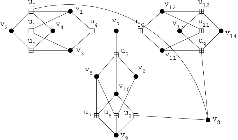
Example IV.3

Figure 12 shows a graph on $m+1$ variable nodes, where the set of all variable nodes except $v_{1}$ form a minimal stopping set of size $m$ , i.e., $s_{\min}=m$ . When $m$ is even, the only irreducible pseudocodewords are of the form $(k,1,1,\ldots,1)$ , where $0\leq k\leq m$ and $k$ is even, and the only nonzero codeword is $(0,1,1,\ldots,1)$ . When $m$ is odd, the irreducible pseudocodewords have the form $(k,1,1,\ldots,1)$ , where $1\leq k\leq m$ , and $k$ is odd, or $(0,2,2,\ldots,2)$ , and the only nonzero codeword is $(1,1,\ldots,1)$ . In general, any pseudocodeword of this graph is a linear combination of these irreducible pseudocodewords. When $k$ is not 0 or 1, then these are irreducible nc-pseudocodewords; the weight vector ${\bf w}=(w_{1},\ldots,w_{m+1})$ , where $w_{1}=-1,w_{2}=+1,$ and $w_{3}=\cdots=w_{m+1}=0$ , shows that these pseudocodewords are bad. When $m$ is even or odd, any reducible pseudocodeword of this graph that includes at least one irreducible nc-pseudocodeword in its sum, is also bad (according to Definition II.9). We also observe that for both the BSC and AWGN channel, all of the irreducible pseudocodewords have weight at most $d_{\min}=m$ or $m+1$ , depending on whether $m$ is even or odd. The minimum pseudocodeword weight is $w_{\min}^{AWGN}=4m/(m+1)$ , and the LDPC constraint graph has a $t$ -value of $m$ .
Figures 14 and 14 show the performance of the code for odd and even $m$ , respectively, on a BIAWGNC with MS, SP, and ML decoding. The performance difference between the MS (respectively, the SP) decoder and the optimal ML decoder is more pronounced for odd $m$ . (In the case of even $m$ , $(0,2,2\dots,2)$ is not a bad pseudocodeword, since it is twice a codeword, unlike in the case for odd $m$ ; thus, one can argue that, relatively, there are a fewer number of bad pseudocodewords when $m$ is even.) Since the graph has low weight bad pseudocodewords, in comparison to the minimum distance, the performance of the MS decoder in the high SNR regime is clearly inferior to that of the ML decoder.

Figure 15 shows the performance of Example 3 for $m=10$ and $m=11$ over the BSC channel with MS iterative decoding. Since there are only $2^{m+1}$ different error patterns possible for the BSC channel, the performance of MS decoding for each error pattern was determined and the average number of output errors were computed. The figure shows that all four-bit or less error patterns were corrected by the MS and the ML decoders. However, the average number of output bit errors for five-bit error patterns with MS decoding was around 0.48 for the $m=11$ code and was around 5.55 for the $m=10$ code, while the ML decoder corrected all five-bit error patterns for both the codes. The average number of output bit errors for six-bit error patterns with MS decoding was 6 for the $m=11$ code and 10.5 for the $m=10$ code, whereas the ML decoder corrected all six bit errors for the $m=11$ code and yielded an average number of output bit errors of 4.545 for the $m=10$ code. The figure also shows that MS decoding is closer to ML decoding for the $m=10$ code than for the $m=11$ code.

This section has demonstrated three particular LDPC constraint graphs having different types of pseudocodewords, leading to different performances with iterative decoding in comparison to optimal decoding. In particular, we observe that the presence of low weight irreducible nc-pseudocodewords, with weight relatively smaller than the minimum distance of the code, can adversely affect the performance of iterative decoding.

V Structure of pseudocodewords

This section examines the structure of lift-realizable pseudocodewords and identifies some sufficient conditions for certain pseudocodewords to potentially cause the min-sum iterative decoder to fail to converge to a codeword. Some of these conditions relate to subgraphs of the base Tanner graph. We recall that we are only considering the set of lift-realizable pseudocodewords and that by Definition II.3, the pseudocodewords have non-negative integer components, and hence are unscaled.

Lemma V.1

Let ${\bf p}=(p_{1},p_{2},\dots,p_{n})$ be a pseudocodeword in the graph $G$ that represents the LDPC code $\mathcal{C}$ . Then the vector ${\bf x}={\bf p}\mbox{ mod }2$ , obtained by reducing the entries in ${\bf p}$ , modulo 2, corresponds to a codeword in $\mathcal{C}$ .

The following implications follow from the above lemma:

•

If a pseudocodeword ${\bf p}$ has at least one odd component, then it has at least $d_{\min}$ odd components.
•

If a pseudocodeword ${\bf p}$ has a support size $|\operatorname{supp}({\bf p})|<d_{\min}$ , then it has no odd components.
•

If a pseudocodeword ${\bf p}$ does not contain the support of any non-zero codeword in its support, then ${\bf p}$ has no odd components.

Lemma V.2

A pseudocodeword ${\bf p}=(p_{1},\dots,p_{n})$ can be written as ${\bf p}={\bf c}^{(1)}+{\bf c}^{(2)}+\dots+{\bf c}^{(k)}+{\bf r}$ , where ${\bf c}^{(1)},\dots,{\bf c}^{(k)}$ , are $k$ (not necessarily distinct) codewords and ${\bf r}$ is some residual vector, not containing the support of any nonzero codeword in its support, that remains after subtracting the codeword vectors ${\bf c}^{(1)},\dots,{\bf c}^{(k)}$ from ${\bf p}$ . Either ${\bf r}$ is the all-zeros vector, or ${\bf r}$ is a vector comprising of $0$ or even entries only.

This lemma describes a particular composition of a pseudocodeword ${\bf p}$ . Note that the above result does not claim that ${\bf p}$ is reducible even though the vector ${\bf p}$ can be written as a sum of codeword vectors ${\bf c}^{(1)},\dots,{\bf c}^{(k)}$ , and ${\bf r}$ . Since ${\bf r}$ need not be a pseudocodeword, it is not necessary that ${\bf p}$ be reducible structurally as a sum of codewords and/or pseudocodewords (as in Definition II.7). It is also worth noting that the decomposition of a pseudocodeword, even that of an irreducible pseudocodeword, is not unique.

Example V.1

For representation B of the $[7,4,3]$ Hamming code as shown in Figure 19 in Section 6, label the vertices clockwise from the top as $v_{1},v_{2},v_{3},v_{4},v_{5},v_{6}$ , and $v_{7}$ . The vector ${\bf p}=(p_{1},\ldots,p_{n})=(1,2,1,1,1,0,2)$ is an irreducible pseudocodeword and may be decomposed as ${\bf p}=(1,0,1,0,0,0,1)+(0,0,0,1,1,0,1)+(0,2,0,0,0,0,0)$ and also as ${\bf p}=(1,0,1,1,1,0,0)+(0,2,0,0,0,0,2)$ . In each of these decompositions, each vector in the sum is a codeword except for the last vector which is the residual vector ${\bf r}$ .

Theorem V.1

Let ${\bf p}=(p_{1},\dots,p_{n})$ be a pseudocodeword. If there is a decomposition of ${\bf p}$ as in Lemma V.2 such that ${\bf r}={\bf 0}$ , then ${\bf p}$ is a good pseudocodeword as in Definition II.8.

Theorem V.2

The following are sufficient conditions for a pseudocodeword ${\bf p}=(p_{1},\dots,p_{n})$ to be bad, as in Definition II.9:

1.

$w^{BSC/AWGN}({\bf p})<d_{\min}$ .
2.

$|\operatorname{supp}({\bf p})|<d_{\min}$ .
3.

If ${\bf p}$ is an irreducible nc-pseudocodeword and $|\operatorname{supp}({\bf p})|\geq\ell+1$ , where $\ell$ is the number of distinct codewords whose support is contained in $\operatorname{supp}({\bf p})$ .

Intuitively, it makes sense for good pseudocodewords, i.e., those pseudocodewords that are not problematic for iterative decoding, to have a weight larger than the minimum distance of the code, $d_{\min}$ . However, we note that bad pseudocodewords can also have weight larger than $d_{\min}$ .

Definition V.1

A stopping set $S$ has property $\Theta$ if $S$ contains at least one pair of variable nodes $u$ and $v$ that are not connected by any path that traverses only via degree two check nodes in the subgraph $G_{|_{S}}$ of $G$ induced by $S$ in $G$ .

Example V.2

In Figure 10 in Section 4, the set $\{v_{1},v_{2},v_{4}\}$ is a minimal stopping set and does not have property $\Theta$ , whereas the set $\{v_{1},v_{3},v_{4},v_{5},v_{6},v_{7},v_{10},v_{11},v_{12},v_{13}\}$ is not minimal but has property $\Theta$ . The graph in Figure 16 is a minimal stopping set that has property $\Theta$ . The graph in Example IV.1 has no minimal stopping sets with property $\Theta$ , and all stopping sets have size at least the minimum distance $d_{\min}$ .

Lemma V.3

Let $S$ be a stopping set in $G$ . Let $t_{S}$ denote the largest component an irreducible pseudocodeword with support $S$ may have in $G$ . If $S$ is a minimal stopping set and does not have property $\Theta$ , then a pseudocodeword with support $S$ has maximal component 1 or 2. That is, $t_{S}=1$ or $2$ .

Subgraphs of the LDPC constraint graph may also give rise to bad pseudocodewords, as indicated below.

Definition V.2

A variable node $v$ in an LDPC constraint graph $G$ is said to be problematic if there is a stopping set $S$ containing $v$ that is not minimal but nevertheless has no proper stopping set $S^{\prime}\subsetneq S$ for which $v\in S^{\prime}$ .

Observe that all graphs in the examples of Section 4 have problematic nodes and conditions 1 and 3 in Theorem V.2 are met in Examples IV.2 and IV.3. The problematic nodes are the variable nodes in the inner ring in Example IV.1, the nodes $v_{7},v_{8}$ in Example IV.2, and $v_{1}$ in Example IV.3. Note that if a graph $G$ has a problematic node, then $G$ necessarily contains a stopping set with property $\Theta$ .

The following result classifies bad nc-pseudocodewords, with respect to the AWGN channel, using the graph structure of the underlying pseudocodeword supports, which, by Lemma II.1, are stopping sets in the LDPC constraint graph.

Theorem V.3

Let $G$ be an LDPC constraint graph representing an LDPC code $\mathcal{C}$ , and let $S$ be a stopping set in $G$ . Then, the following hold:

1.

If there is no non-zero codeword in $\mathcal{C}$ whose support is contained in $S$ , then all nc-pseudocodewords of $G$ , having support equal to $S$ , are bad as in Definition II.9. Moreover, there exists a bad pseudocodeword in $G$ with support equal to $S$ .
2.
If there is at least one codeword ${\bf c}$ whose support is contained in $S$ , then we have the following cases:
1. (a)
  if $S$ is minimal,
  1. (i)
    
    there exists a nc-pseudocodeword ${\bf p}$ with support equal to $S$ iff $S$ has property $\Theta$ .
  2. (ii)
    
    all nc-pseudocodewords with support equal to $S$ are bad.
2. (b)
  if $S$ is not minimal,
  1. (i)
    
    and $S$ contains a problematic node $v$ such that $v\notin S^{\prime}$ for any proper stopping set²² 2 A proper stopping set $S^{\prime}$ of $S$ is a non-empty stopping set that is a strict subset of $S$ . $S^{\prime}\subsetneq S$ , then there exists a bad pseudocodeword ${\bf p}$ with support $S$ . Moreover, any irreducible nc-pseudocodeword ${\bf p}$ with support $S$ is bad.
  2. (ii)
    
    and $S$ does not contain any problematic nodes, then every variable node in $S$ is contained in a minimal stopping set within $S$ . Moreover, there exists a bad nc-pseudocodeword with support $S$ iff either one of these minimal stopping sets is not the support of any non-zero codeword in $\mathcal{C}$ or one of these minimal stopping sets has property $\Theta$ .

The graph in Figure 17 is an example of case 2(b)(ii) in Theorem V.3. Note that the stopping set in the figure is a disjoint union of two codeword supports and therefore, there are no irreducible nc-pseudocodewords.

The graph in Figure 18 is an example of case 2(a). The graph has property $\Theta$ and therefore has nc-pseudocodewords, all of which are bad.

V-A Remarks on the weight vector and channels

In [6], Frey et. al show that the max-product iterative decoder (equivalently, the MS iterative decoder) will always converge to an irreducible pseudocodeword (as in Definition II.7) on the AWGN channel. However, their result does not explicitly show that for a given irreducible pseudocodeword ${\bf p}$ , there is a weight vector ${\bf w}$ such that the cost ${\bf p}{\bf w}^{T}$ is the smallest among all possible pseudocodewords. In the previous subsection, we have given sufficient conditions under which such a weight vector can explicitly be found for certain irreducible pseudocodewords. We believe, however, that finding such a weight vector ${\bf w}$ for any irreducible pseudocodeword ${\bf p}$ may not always be possible. In particular, we state the following definitions and results.

Definition V.3

A truncated AWGN channel, parameterized by $L$ and denoted by $TAWGN(L)$ , is an AWGN channel whose output log-likelihood ratios corresponding to the received values from the channel are truncated, or limited, to the interval $[-L,L]$ .

In light of [15, 16], we believe that there are fewer problematic pseudocodewords on the BSC than on the truncated AWGN channel or the AWGN channel.

Definition V.4

For an LDPC constraint graph $G$ that defines an LDPC code $\mathcal{C}$ , let $P^{B}_{AWGN}(G)$ be the set of lift-realizable pseudocodewords of $G$ where for each pseudocodeword ${\bf p}$ in the set, there exists a weight vector ${\bf w}$ such that the cost ${\bf p}{\bf w}^{T}$ on the AWGN channel is the smallest among all possible lift-realizable pseudocodewords in $G$ .

Let $P^{B}_{BSC}(G)$ and $P^{B}_{TAWGN(L)}(G)$ be defined analogously for the BSC and the truncated AWGN channel, respectively. Then, we have the following result:

Theorem V.4

For an LDPC constraint graph $G$ , and $L\geq 1$ , we have

P^{B}_{BSC}(G)\subseteq P^{B}_{TAWGN(L)}(G)\subseteq P^{B}_{AWGN}(G).

The above result says that there may be fewer problematic irreducible pseudocodewords for the BSC than over the TAWGN(L) channel and the AWGN channel. In other words, the above result implies that MS iterative decoding may be more accurate for the BSC than over the AWGN channel. Thus, quantizing or truncating the received information from the channel to a smaller interval before performing MS iterative decoding may be beneficial. (Note that while the above result considers all possible weight vectors that can occur for a given channel, it does not take into account the probability distribution of weight vectors for the different channels, which is essential when comparing the performance of MS decoding across different channels.) Since the set of lift-realizable pseudocodewords for MS iterative decoding is the set of pseudocodewords for linear-programming (LP) decoding (see Section 2), the same analogy carries over to LP decoding as well. Indeed, at high enough signal to noise ratios, the above observation has been shown true for the case of LP decoding in [15] and more recently in [16].

VI Graph Representations and Weight Distribution

In this section, we examine different representations of individual LDPC codes and analyze the weight distribution of lift-realizable pseudocodewords in each representation and how it affects the performance of the MS iterative decoder. We use the classical $[7,4,3]$ and $[15,11,3]$ Hamming codes as examples.

Figure 19 shows three different graph representations of the $[7,4,3]$ Hamming code. We will call the representations $A$ , $B$ , and $C$ , and moreover, for convenience, also refer to the graphs in the three respective representations as $A$ , $B$ , and $C$ . The graph $A$ is based on the systematic parity check matrix representation of the $[7,4,3]$ Hamming code and hence, contains three degree one variable nodes, whereas the graph $B$ has no degree one nodes and is more structured (it results in a circulant parity check matrix) and contains 4 redundant check equations compared to $A$ , which has none, and $C$ , which has one. In particular, $A$ and $C$ are subgraphs of $B$ , with the same set of variable nodes. Thus, the set of lift-realizable pseudocodewords of $B$ is contained in the set of lift-realizable pseudocodewords of $A$ and $C$ , individually. Hence, $B$ has fewer number of lift-realizable pseudocodewords than $A$ or $C$ . In particular, we state the following result:

Theorem VI.1

The number of lift-realizable pseudocodewords in an LDPC graph $G$ can only reduce with the addition of redundant check nodes to $G$ .

The proof is obvious since with the introduction of new check nodes in the graph, some previously valid pseudocodewords may not satisfy the new set of inequality constraints imposed by the new check nodes. (Recall that at a check node $c$ having variable node neighbors $v_{i_{1}},\dots,v_{i_{k}}$ , a pseudocodeword ${\bf p}=(p_{1},\dots,p_{n})$ , must satisfy the following inequalities $p_{i_{j}}\leq\sum_{h\neq j,h=1,\dots,k}p_{i_{h}},\mbox{ for }j=1,\dots,k$ (see equation (1)).) However, the set of valid codewords in the graph remains the same, since we are introducing only redundant (or, linearly dependent) check nodes. Thus, a graph with more check nodes can only have fewer number of lift-realizable pseudocodewords and possibly a better pseudocodeword-weight distribution.

If we add all possible redundant check nodes to the graph, which, we note, is an exponential number in the number of linearly dependent rows of the parity check matrix of the code, then the resulting graph would have the smallest number of lift-realizable pseudocodewords among all possible representations of the code. If this graph does not have any bad nc-pseudocodewords (both lift-realizable ones and those arising on the computation tree) then the performance obtained with iterative decoding is the same as the optimal ML performance.

Remark VI.1

Theorem VI.1 considers only the set of lift-realizable pseudocodewords of a Tanner graph. On adding redundant check nodes to a Tanner graph, the shape of the computation tree is altered and thus, it is possible that some new pseudocodewords arise in the altered computation tree, which can possibly have an adverse effect on iterative decoding. The $[4,1,4]$ repetition code example from Section 2.C illustrates this. Iterative decoding is optimal on the single cycle representation of this code. However, on adding a degree four redundant check node, the iterative decoding performance deteriorates due to the introduction of bad pseudocodewords to the altered computation tree. (See Figure 7.) (The set of lift-realizable pseudocodewords however remains the same for the new graph with redundant check nodes as for the original graph.)

Returning to the Hamming code example, graph $B$ can be obtained by adding edges to either $A$ or $C$ , and thus, $B$ has more cycles than $A$ or $C$ . The distribution of the weights of the irreducible lift-realizable pseudocodewords for the three graphs $A$ , $B$ , and $C$ is shown³³ 3 The plots considered all pseudocodewords in the three graphs that had a maximum component value of at most 3. Hence, for each codeword ${\bf c}$ , ${2\bf c}$ and ${3\bf c}$ are also counted in the histogram, and each has weight at least $d_{\min}$ . However, each irreducible nc-pseudocodeword ${\bf p}$ is counted only once, as ${\bf p}$ contains at least one entry greater than 1, and any nonzero multiple of ${\bf p}$ would have a component greater than 3. The $t$ -value (see Section 5) is 3 for the graphs $A$ , $B$ , and $C$ of the $[7,4,3]$ Hamming code. in Figure 20. (The distribution considers all irreducible pseudocodewords in the graph, since irreducible pseudocodewords may potentially prevent the MS decoder to converge to any valid codeword [6].) Although, all three graphs have a pseudocodeword of weight three⁴⁴ 4 Note that this pseudocodeword is a valid codeword in the graph and is thus a good pseudocodeword for iterative decoding., Figure 20 shows that $B$ has most of its lift-realizable pseudocodewords of high weight, whereas $C$ , and more particularly, $A$ , have more low-weight lift-realizable pseudocodewords. The corresponding weight distributions over the BEC and the BSC channels are shown in Figure 21. $B$ has a better weight distribution than $A$ and $C$ over these channels as well.

The performance of MS iterative decoding of $A$ , $B$ , and $C$ on the BIAWGNC with signal to noise ratio $E_{b}/N_{o}$ is shown in Figures 25, 25, and 25, respectively. (The maximum number of decoding iterations was fixed at 100.) The performance plots show both the bit error rate and the frame error rate, and further, they also distinguish between undetected decoding errors, that are caused due to the decoder converging to an incorrect but valid codeword, and detected errors, that are caused due to the decoder failing to converge to any valid codeword within the maximum specified number of decoding iterations, 100 in this case. The detected errors can be attributed to the decoder trying to converge to an nc-pseudocodeword rather than to any valid codeword.

Representation $A$ has a significant detected error rate, whereas representation $B$ shows no presence of detected errors at all. All errors in decoding $B$ were due to the decoder converging to a wrong codeword. (We note that an optimal ML decoder would yield a performance closest to that of the iterative decoder on representation $B$ .) This is interesting since the graph $B$ is obtained by adding 4 redundant check nodes to the graph $A$ . The addition of these 4 redundant check nodes to the graph removes most of the low-weight nc-pseudocodewords that were present in $A$ . (We note here that representation $B$ includes all possible redundant parity-check equations there are for the [7,4,3] Hamming code.) Representation $C$ has fewer number of pseudocodewords compared to $A$ . However, the set of irreducible pseudocodewords of $C$ is not a subset of the set of irreducible pseudocodewords of $A$ . The performance of iterative decoding on representation $C$ indicates a small fraction of detected errors.

Figure 25 compares the performance of min-sum decoding on the three representations. Clearly, $B$ , having the best pseudocodeword weight distribution among the three representations, yields the best performance with MS decoding, with performance almost matching that of the optimal ML decoder.

Figure 26 shows the performance of the three different representations over the BSC channel with MS iterative decoding. Since there are only $2^{7}=128$ different error patterns, the performance of MS decoding for each error pattern was determined and the average number of output errors were computed. Representations A and C failed to correct any non-zero error pattern whereas representation B corrected all one-bit error patterns. The performance of MS decoding using representation B was identical to the performance of the ML decoder and the MS decoder always converged to the ML codeword with representation B. This goes to show that representation B is in fact the optimal representation for the BSC channel.

Similarly, we also analyzed three different representations of the $[15,11,3]$ Hamming code. Representation $A$ has its parity check matrix in the standard systematic form and thus, the corresponding Tanner graph has 4 variable nodes of degree one. Representation $B$ includes all possible redundant parity check equations of representation $A$ and has the best pseudocodeword-weight distribution. Representation $C$ includes up to order-two redundant parity check equations from the parity check matrix of representation $A$ , meaning, the parity check matrix of representation $C$ contained all linear combinations of every pair of rows in the parity check matrix of representation $A$ . Thus, its (lift-realizable) pseudocodeword-weight distribution is superior to that of $A$ but inferior to that of $B$ . (See Figure 30.)

The analogous performance of MS iterative decoding of representations $A$ , $B$ , and $C$ of the $[15,11,3]$ Hamming code on a BIAWGNC with signal to noise ratio $E_{b}/N_{o}$ is shown in Figures 30, 30, and 30, respectively. (The maximum number of decoding iterations was fixed at 100.) We observe similar trends in the performance curves as in the previous example. $A$ shows a prominent detected error rate, whereas $B$ and $C$ show no presence of detected errors at all. The results suggest that merely adding order two redundant check nodes to the graph of $A$ is sufficient to remove most of the low-weight pseudocodewords.

Inferring from the empirical results of this section, we comment that LDPC codes that have structure and redundant check nodes, for example, the class of LDPC codes obtained from finite geometries [17], are likely to have fewer number of low-weight pseudocodewords in comparison to other randomly constructed LDPC graphs of comparable parameters. Despite the presence of a large number of short cycles (i.e., 4-cycles and 6-cycles), the class of LDPC codes in [17] perform very well with iterative decoding. It is worth investigating how the set of pseudocodewords among existing LDPC constructions can be improved, either by adding redundancy or modifying the Tanner graphs, so that the number of (bad) pseudocodewords, both lift-realizable ones as well as those occurring on the computation tree, is lowered.

VII Conclusions

This paper analyzed pseudocodewords of Tanner graphs, with the focus on the structure, bounds on the minimum pseudocodeword weight, and iterative decoding performance. It would be worthwhile to relate the results in Section 6 to the stopping redundancy, as introduced in [18]. Since this paper primarily dealt with lift-realizable pseudocodewords, the results presented are also applicable in the analysis of LP decoding. We hope the insights gained from this paper will aid in the design of LDPC codes with good minimum pseudocodeword weights.

Acknowledgments

We thank Joachim Rosenthal, Pascal Vontobel, and the two reviewers for their careful reading of the paper and their insightful comments which have considerably improved this paper. We also thank Reviewer 1 for providing an elegant proof of Theorem III.5.

References

[1] N. Wiberg, Codes and Decoding on General Graphs. PhD thesis, University of Link $\ddot{o}$ ping, Sweden, 1996.
[2] G. A. Horn, Iterative Decoding and Pseudocodewords. PhD thesis, California Institute of Technology, Pasadena, CA, USA, 1999.
[3] G. D. Forney, Jr., “The forward-backward algorithm,” in Proccedings of the 34^th Annual Allerton Conference on Communications, Control, and Computing, (Monticello, Illinois, USA), pp. 432–446, October 1996.
[4] G. D. Forney, Jr., R. Koetter, F. R. Kschischang, and A. Reznik, On the effective weights of pseudocodewords for codes defined on graphs with cycles, vol. 123, ch. 5, pp. 101–112. IMA Volumes in Mathematics and its Applications, 2001.
[5] R. Koetter and P. O. Vontobel, “Graph-covers and iterative decoding of finite length codes,” in Proceedings of the IEEE International Symposium on Turbo Codes and Applications, (Brest, France), Sept. 2003.
[6] B. J. Frey, R. Koetter, and A. Vardy, “Signal-space characterization of iterative decoding,” IEEE Transactions on Information Theory, vol. IT-47, pp. 766–781, Feb 2001.
[7] J. Feldman, Decoding Error-Correcting Codes via Linear Programming. PhD thesis, Massachusetts Institute of Technology, Cambridge, MA, USA, 2003.
[8] R. G. Gallager, Low-Density Parity Check Codes. Cambridge, MA: M.I.T. Press, 1963.
[9] R. Koetter, W.-C. W. Li, P. O. Vontobel, and J. L. Walker, “Pseudo-codewords of cycle codes via zeta functions,” in Proceedings of 2004 IEEE Information Theory Workshop, (San Antonio, USA), October 2004.
[10] T. D. Coleman, “Pseudocodewords presentation.” Technical Report, M.I.T., Cambridge, MA, Sept. 23 2003.
[11] C. Di, D. Proietti, I. Teletar, T. Richardson, and R. Urbanke, “Finite-length analysis of low-density parity-check codes on the binary erasure channel,” IEEE Transactions on Information Theory, vol. IT-48, pp. 1570–1579, June 2002.
[12] F. R. Kschischang, B. J. Frey, and H. A. Loeligar, “Factor graphs and the sum-product algorithm,” IEEE Transaction in Information Theory, vol. IT-47, no. 2, pp. 498–519, Feb. 2001.
[13] R. M. Tanner, “A recursive approach to low complexity codes,” IEEE Transactions on Information Theory, vol. IT-27, no. 5, pp. 533–547, Sept. 1981.
[14] A. Orlitsky, R. Urbanke, K. Vishwanathan, and J. Zhang, “Stopping sets and the girth of Tanner graphs,” in Proceedings of 2002 IEEE International Symposium on Information Theory, (Lausanne, Switzerland), p. 2, June 30 - July 5 2002.
[15] J. Feldman and C. Stein, “LP decoding achieves capacity,” in Symposium on Discrete Algorithms (SODA), (Vancouver, Canada), Jan 23 – 25 2005.
[16] J. Feldman, R. Koetter, and P. O. Vontobel, “The benefits of thresholding in LP decoding of LDPC codes,” in Proceedings of 2005 IEEE International Symposium on Information Theory, (Adelaide, Australia), Sept. 4 – 9 2005.
[17] Y. Kou, S. Lin, and M. P. C. Fossorier, “Low density parity-check codes based on finite geometries: A rediscovery and new results,” IEEE Transactions on Information Theory, vol. IT-47, no. 7, pp. 2711–2736, Nov. 2001.
[18] M. Schwartz and A. Vardy, “On the stopping distance and the stopping redundancy of codes,” Submitted to IEEE Transactions on Information Theory, March 2005.
[19] C. Kelley, D. Sridhara, J. Xu, and J. Rosenthal, “Pseudocodeword weights and stopping sets,” in Proceedings of 2004 IEEE International Symposium on Information Theory, (Chicago, USA), p. 150, June 27 - July 3 2004.
[20] J. L. Gross and T. W. Tucker, Topological Graph Theory. Wiley, New York, 1987.
[21] S. M. Aji and R. J. McEliece, “The generalized distributive law,” IEEE Transactions on Information Theory, vol. IT-46, no. 2, pp. 325–343, March 2000.
[22] C. Kelley and D. Sridhara, “Structure of pseudocodewords in Tanner graphs,” in Proceedings of 2004 International Symposium on Information Theory and its Applications, (Parma, Italy), p. CDROM, October 10–13 2004.
[23] P. O. Vontobel and R. Koetter, “On the relationship between linear programming decoding and min-sum algorithm decoding,” in Proceedings of 2004 International Symposium on Information Theory and its Applications, (Parma, Italy), p. CDROM, October 10–13 2004.

Proof of Lemma II.1: Consider the subgraph $G_{|S}$ of $G$ induced by the set of vertices $S=\operatorname{supp}({\bf p})$ . Observe that every cloud of check nodes in the corresponding cover of $G_{|S}$ is connected to either none or at least two of the variable clouds in the support of ${\bf p}$ . If this were not the case, then there would be a cloud of check nodes in the cover with at least one check node in that cloud connected to exactly one variable node of bit value one, thus, leaving the check node constraint unsatisfied. Therefore, the corresponding variable nodes in the base graph $G$ satisfy the conditions of a stopping set. $\hfill\IEEEQEDclosed$

Proof of Claim II.1: Let $G$ represent the constraint graph of an LDPC code $\mathcal{C}$ . Suppose $G$ is a tree, then clearly, any pseudocodeword of $G$ can be expressed as a linear combination of codewords of $G$ . Hence, suppose $G$ is not a tree, and suppose all check nodes in $G$ are of degree two. Then the computation tree contains only check nodes of degree two and hence, for a valid assignment on the computation tree, the value of any child variable node $v_{1}$ on the computation tree that stems from a parent check node $u$ is the same as the value of the variable node $v_{2}$ which is the parent node of $u$ . Thus, the only local codeword configurations at each check node is the all-ones configurations when the root node of the tree is assigned the value one. Hence, the only valid solutions on the computation tree correspond to the all ones vector and the all zeros vector – which are valid codewords in $\mathcal{C}$ .
Conversely, suppose $G$ is not a tree and suppose there is a check node $u$ of degree $k$ in $G$ . Let $v_{1},v_{2},\dots,v_{k}$ be the variable node neighbors of $u$ . Enumerate the computation tree rooted at $v_{1}$ for a sufficient depth such that the node $u$ appears several times in the tree and also as a node in the final check node layer of the tree. Then there are several possible valid assignments in the computation tree, where the values assigned to the leaf nodes that stem from $u$ yield a solution that is not a valid codeword in $G$ . Thus, $G$ contains irreducible nc-pseudocodewords on its computation tree. $\hfill\IEEEQEDclosed$

Proof of Claim II.2: Let $G$ represent the constraint graph of an LDPC code $\mathcal{C}$ . Suppose $G$ is a tree, then clearly, any pseudocodeword of $G$ can be expressed as a linear combination of codewords of $G$ . Hence, suppose $G$ is not a tree, and between every pair of variable nodes in $G$ there is a path that contains only degree two check nodes in $G$ . Then $G$ contains only lift-realizable pseudocodewords of the form $(k,k,\dots,k)$ , where $k$ is a positive integer. Hence, the only irreducible pseudocodewords in $G$ are the all-zeros vector $(0,0,\dots,0)$ and either the all-ones vector $(1,1,\dots,1)$ or the all-twos vector $(2,2,\dots,2)$ (if the all-ones vector is not a codeword in $G$ ). $\hfill\IEEEQEDclosed$

Proof of Theorem III.1:

Case: $\frac{g}{2}$ odd. At a single constraint node, the following inequality holds (see equation 1):

\alpha_{i}\leq\sum_{j\neq i}\alpha_{j}

Applying this inequality in the LDPC constraint graph enumerated as a tree with the root node corresponding to the dominant pseudocodeword component $\alpha_{1}$ , we have

d\alpha_{1}\leq\sum_{j\in L_{0}}\alpha_{j},

where $L_{0}$ corresponds to variable nodes in the first level (level 0) of the tree. Similarly, we have

d(d-1)\alpha_{1}\leq\sum_{j\in L_{1}}\alpha_{j},

and so on, until,

d(d-1)^{\frac{g-6}{4}}\alpha_{1}\leq\sum_{j\in L_{\frac{g-6}{4}}}\alpha_{j}

Since the LDPC graph has girth $g$ , the variable nodes up to level $L_{\frac{g-6}{4}}$ ⁵⁵ 5 Note that $L_{i}$ refers to the level for which the exponent of the $(d-1)$ term is $i$ . are all distinct. The above inequalities yield:

{\left[1+d+d(d-1)+\cdots+d(d-1)^{\frac{g-6}{4}}\right]\alpha_{1}\leq\sum_{i\in\{1\}\cup L_{0}\cup\dots L_{\frac{g-6}{4}}}\alpha_{i}}{\leq\sum_{all}\alpha_{i}}

Without loss of generality, let us assume, $\alpha_{1}\geq\alpha_{2}\geq\dots\geq\alpha_{e}$ to be the $e$ dominant components in ${\bf p}$ . That is, $\alpha_{1}+\alpha_{2}+\cdots+\alpha_{e}\geq\frac{\sum_{i}\alpha_{i}}{2}$ . Since, each is at most $\alpha_{1}$ , we have ${{\sum_{i=1}^{e}\alpha_{i}\leq e\alpha_{1}.}}$ This implies that

{e\alpha_{1}\geq\sum_{i=1}^{e}\alpha_{i}\geq\sum_{i}\frac{\alpha_{i}}{2}}{\geq\frac{\left[1+d+d(d-1)+\cdots+d(d-1)^{\frac{g-6}{4}}\right]\alpha_{1}}{2}}

{\Rightarrow e\geq\frac{\left[1+d+d(d-1)+\cdots+d(d-1)^{\frac{g-6}{4}}\right]}{2}}.

Since ${w}_{BSC}=2e$ , the result follows. (The case when $\frac{g}{2}$ is even is treated similarly.)

AWGN case: Let $x=\frac{\left[1+d+d(d-1)+\cdots+d(d-1)^{\frac{g-6}{4}}\right]}{2}$ . Since,

\sum_{i=1}^{e}\alpha_{i}\geq\frac{\left[1+d+d(d-1)+\cdots+d(d-1)^{\frac{g-6}{4}}\right]\alpha_{1}}{2},

we can write ${\sum_{i=1}^{e}\alpha_{i}=(x+y)\alpha_{1}},$ where $y$ is some non-negative quantity. Suppose $\alpha_{1}+\cdots+\alpha_{e}=\alpha_{e+1}+\cdots\alpha_{n}$ .

Then, since we have $\sum_{i=1}^{n}\alpha_{i}^{2}\leq 2\sum_{i=1}^{e}\alpha_{i}^{2}\leq 2\alpha_{1}(\sum_{i=1}^{e}\alpha_{i})=2(x+y)\alpha_{1}^{2}$ ., we get,

{w=\frac{(\sum_{i=1}^{n}\alpha_{i})^{2}}{\sum_{i=1}^{n}\alpha_{i}^{2}}}{\geq\frac{(2\sum_{i=1}^{e}\alpha_{i})^{2}}{2\sum_{i=1}^{e}\alpha_{i}^{2}}}

{w\geq\frac{4(x+y)^{2}\alpha_{1}^{2}}{2(x+y)\alpha_{1}^{2}}=2(x+y)}{\geq 2x.}

(The case $\alpha_{1}+\cdots+\alpha_{e}>\alpha_{e+1}+\cdots\alpha_{n}$ is treated similarly.) $\hfill\IEEEQEDclosed$

Proof of Theorem III.2: As in the proof of Theorem III.1, where we note that for a single constraint with neighbors having pseudocodeword components $\alpha_{1},\dots,\alpha_{k}$ , we have the following relation (for $\alpha_{i},i=1,\dots,k$ ):

(\epsilon k)\alpha_{i}\leq\sum_{j=1}^{k}\alpha_{j}.

The result follows by applying this inequality at every constraint node as in the proof of Theorem III.1. $\hfill\IEEEQEDclosed$

Proof of Lemma III.1: Let ${\bf p}=(\alpha_{1},\dots,\alpha_{n})$ be a pseudocodeword of $G$ , and without loss of generality, let $\alpha_{1}\geq\alpha_{2}\geq\ldots\geq\alpha_{n}$ . To establish the inequality for the AWGN channel, we need to show

\frac{(\sum_{i=1}^{n}\alpha_{i})^{2}}{\sum_{i=1}^{n}\alpha_{i}^{2}}\geq\frac{\sum_{i=1}^{n}\alpha_{i}}{\max_{i}\alpha_{i}}=\frac{\sum_{i=1}^{n}\alpha_{i}}{\alpha_{1}}.

Since $\sum_{i}\alpha_{i}^{2}\leq\alpha_{1}^{2}+\alpha_{1}\alpha_{2}+\cdots+\alpha_{1}\alpha_{n}=\alpha_{1}(\sum_{i}\alpha_{i})$ , this implies

\frac{(\sum_{i=1}^{n}\alpha_{i})^{2}}{\sum_{i=1}^{n}\alpha_{i}^{2}}\geq\frac{(\sum_{i=1}^{n}\alpha_{i})^{2}}{\alpha_{1}\sum_{i=1}^{n}\alpha_{i}}\geq\frac{\sum_{i=1}^{n}\alpha_{i}}{\alpha_{1}}.

Hence, $w^{AWGN}({\bf p})\geq w_{\mathrm{max-frac}}({\bf p})$ .
To establish the bound for the BSC, let $e$ be the smallest number such that $\sum_{i=1}^{e}\alpha_{i}\geq\frac{\sum_{i=1}^{n}\alpha_{i}}{2}$ . First suppose $\sum_{i=1}^{e}\alpha_{i}=\sum_{i=e+1}^{n}\alpha_{i}$ . Then $w^{BSC}({\bf p})=2e$ . Moreover, $w_{\mathrm{max-frac}}({\bf p})=\frac{\sum_{i=1}^{n}\alpha_{i}}{\alpha_{1}}=\frac{2\sum_{i=1}^{e}\alpha_{i}}{\alpha_{1}}$ . Each $\alpha_{i}\leq\alpha_{1}\Rightarrow w_{\mathrm{max-frac}}({\bf p})\leq\frac{2e\alpha_{1}}{\alpha_{1}}=2e=w^{BSC}({\bf p})$ . Now suppose $\sum_{i=1}^{e}\alpha_{i}>\sum_{i=e+1}^{n}\alpha_{i}$ . Then, for some $\delta>0$ , we have $\sum_{i=1}^{e}\alpha_{i}=\sum_{i=e+1}^{n}\alpha_{i}+\delta$ . We have $w_{\mathrm{max-frac}}({\bf p})=\frac{\sum_{i=1}^{n}\alpha_{i}}{\alpha_{1}}=\frac{\sum_{i=1}^{e}\alpha_{i}+\sum_{i=e+1}^{n}\alpha_{i}}{\alpha_{1}}$ . Note that $\sum_{i=1}^{e}\alpha_{i}+\sum_{i=e+1}^{n}\alpha_{i}<2\sum_{i=1}^{e}\alpha_{i}<(2e)\alpha_{1}$ . Thus, $w_{\mathrm{max-frac}}({\bf p})<\frac{2e\alpha_{1}}{\alpha_{1}}=2e$ . $\hfill\IEEEQEDclosed$

Proof of Corollary III.4: Follows from Lemma III.1 and Theorem III.3. $\hfill\IEEEQEDclosed$

Proof of Theorem III.5: In the polytope representation introduced by Koetter and Vontobel in [5], irreducible pseudocodewords correspond to the edges of the fundamental cone, which can be described by $\{{\bf x}\ |\ x_{i}\geq 0,i=1,\ldots,n\}$ and $\{{\bf x}\ |\ x_{i}\leq\sum_{i^{\prime}\in N(j)\backslash\{i\}}x_{i^{\prime}}\}$ for all check nodes $j$ and all variable nodes $i$ in $N(j)$ . Consider the polytope that is the intersection of the fundamental cone with the hyperplane $x_{1}+\cdots+x_{n}=1$ . The vertices of this polytope have a one-to-one correspondence with the edges of the fundamental cone. Let $v$ be a fixed vertex of this new polytope. Then $v$ satisfies at least $n-1$ of the above inequalities with equality. Together with the hyperplane equality, $v$ meets at least $n$ inequalities with equality. The resulting system of linear equations contains only integers as coefficients. By Cramer’s rule, the vertex $v$ must have rational coordinates. Taking the least common multiple of all denominators of all coordinates of all vertices gives an upper bound on $t$ . Therefore, $t$ is finite. $\hfill\IEEEQEDclosed$

Proof of Theorem III.6: Let $m$ be the minimum degree lift needed to realize the given pseudocodeword ${\bf p}$ . Then, in a degree $m$ lift graph $\hat{G}$ that realizes ${\bf p}$ , the maximum number of active check nodes in any check cloud is at most $m$ . A check cloud $u$ is connected to $\sum_{i\in N(u)}p_{i}$ active variable nodes from the variable clouds adjoining check cloud $u$ . (Note that $N(u)$ represents all the variable clouds adjoining $u$ .) Since every active check node in any check cloud has at least two (an even number) active variable nodes connected to it, we have that $2m\leq max_{u}\sum_{i\in N(u)}p_{i}$ . This quantity can be upper-bounded by $td_{r}^{+}$ since $p_{i}\leq t$ , for all $i$ , and $|N(u)|\leq d_{r}^{+}$ , for all $u$ . $\hfill\IEEEQEDclosed$

Proof of Lemma III.2: (a) AWGN case: Let $n_{k}$ be the number of $p_{i}$ ’s that are equal to $k$ , for $k=1,\dots,t$ . The pseudocodeword weight is then equal to:

w^{AWGN}({\bf p})=\frac{(n_{1}+2n_{2}+\dots+tn_{t})^{2}}{(n_{1}+2^{2}n_{2}+\dots+t^{2}n_{t})}.

Now, we have to find a number $r$ such that $w^{AWGN}({\bf p})\geq r|\operatorname{supp}({\bf p})|$ . Note however, that $|\operatorname{supp}({\bf p})|=n_{1}+n_{2}+\cdots+n_{t}$ . This implies that for an appropriate choice of $r$ , we have

\frac{(n_{1}+2n_{2}+\cdots+tn_{t})^{2}}{(n_{1}+2^{2}n_{2}+\cdots+t^{2}n_{t})}\geq r(n_{1}+\cdots n_{t})\mbox{\hskip 7.22743pt or \hskip 7.22743pt}\sum_{i=1}^{t}i^{2}n_{i}^{2}\geq\sum_{i=1}^{t}\sum_{j=i+1}^{t}\frac{(i^{2}+j^{2})r-2ij}{1-r}n_{i}n_{j}\hskip 7.22743pt(*)

Note that $r<1$ in the above. Clearly, if we set $r$ to be the minimum over all $1\leq i<j\leq n$ such that $(i^{2}+j^{2})r\leq 2ij$ , then it can be verified that this choice of $r$ will ensure that $(*)$ is true. This implies $r=\frac{2t}{1+t^{2}}$ (for $i=1,j=t$ ).

However, observe that left-hand-side (LHS) in $(*)$ can be written as the following LHS:

\frac{1}{t-1}\sum_{i=1}^{t}\sum_{j=i+1}^{t}(i^{2}n_{i}^{2}+j^{2}n_{j}^{2})\geq\sum_{i=1}^{t}\sum_{j=i+1}^{t}\frac{(i^{2}+j^{2})r-2ij}{1-r}n_{i}n_{j}

Now, using the inequality $a^{2}+b^{2}\geq 2ab$ , $r$ can be taken as the minimum over all $1\leq i<j\leq t$ such that $\frac{1}{t-1}(i^{2}n_{i}^{2}+j^{2}n_{j}^{2})\geq\frac{r(i^{2}+j^{2})-2ij}{1-r}n_{i}n_{j}$ . The smallest value of $r$ for which this inequality holds for all $1\leq i<j\leq t$ is given by $r=\frac{2t^{2}}{(1+t^{2})(t-1)+2t}$ , thereby proving the lemma in the AWGN case.

BSC case:

Since $w^{BSC}({\bf p})\geq w_{\mathrm{max-frac}}({\bf p})$ , we have from Lemma III.1 that $w^{BSC}({\bf p})\geq\frac{p_{1}+\cdots+p_{n}}{\max p_{i}}\geq\frac{|\operatorname{supp}({\bf p})|}{t}$ . (Note that the $p_{i}$ ’s are non-negative integers.) Therefore, $w^{BSC}({\bf p})\geq\frac{1}{t}|\operatorname{supp}({\bf p})|$ . $\hfill\IEEEQEDclosed$

Proof of Theorem III.8: Let ${\bf p}$ be a good pseudocodeword. This means that if for any weight vector ${\bf w}$ we have ${\bf c}{\bf w}^{T}\geq 0$ for all ${\bf 0}\neq{\bf c}\in C$ , then, ${\bf p}{\bf w}^{T}\geq 0$ . Let us now consider the BSC and the AWGN cases separately.

BSC case: Suppose at most $\frac{d_{\min}}{2}$ errors occur in channel. Then, the corresponding weight vector ${\bf w}$ will have $\frac{d_{\min}}{2}$ or fewer components equal to $-1$ and the remaining components equal to $+1$ . This implies that the cost of any ${\bf 0}\neq{\bf c}\in C$ (i.e., ${\bf c}{\bf w}^{T}$ ) is at least $0$ since there are at least $d_{\min}$ $1$ ’s in support of any ${\bf 0}\neq{\bf c}\in C$ . Since ${\bf p}$ is a good pseudocodeword, it must also have positive cost, i.e. ${\bf p}{\bf w}^{T}\geq 0$ . Let us assume that the $-1$ ’s occur in the dominant $\frac{d_{\min}}{2}$ positions of ${\bf p}$ , and without loss of generality, assume $p_{1}\geq p_{2}\geq\ldots\geq p_{n}$ . (Therefore, ${\bf w}=(-1,-1,\dots,-1,+1,+1,\dots,+1)$ .) Positive cost of ${\bf p}$ implies $p_{1}+\cdots+p_{d_{\min}/2}\leq p_{(d_{\min}/2)+1}+\cdots+p_{n}$ . So we have $e\geq\frac{d_{\min}}{2}$ , where $e$ is as defined in the pseudocodeword weight of $p$ for the BSC. The result follows.

AWGN case: Without loss of generality, let $p_{1}$ be dominant component of ${\bf p}$ . Set the weight vector ${\bf w}=(1-d_{\min},1,\ldots,1)$ . Then it can be verified that ${\bf c}{\bf w}^{T}\geq{\bf 0}$ for any ${\bf 0}\neq{\bf c}\in C$ . Since ${\bf p}$ is a good pseudocodeword, this implies ${\bf p}$ also must have positive cost. Cost of ${\bf p}$ is $(1-d_{\min})p_{1}+p_{2}+\cdots+p_{n}\geq 0\Rightarrow d_{\min}\leq\frac{p_{1}+\cdots+p_{n}}{p_{1}}$ . Note that the right-hand-side (RHS) is $w_{\mathrm{max-frac}}({\bf p})$ ; hence, the result follows from Lemma III.1.

Now let us consider ${\bf p}$ to be a bad pseudocodeword. From Lemma II.1, we have $|\operatorname{supp}({\bf p})|\geq s_{\min}$ . Therefore, $w_{\mathrm{max-frac}}({\bf p})\geq\frac{s_{\min}}{t}$ (since $p_{1}=t$ is the maximum component of ${\bf p}$ ), and hence, the result follows by Lemmas III.1 and III.2. $\hfill\IEEEQEDclosed$

Proof of Lemma V.1: Consider a graph $H$ having a single check node which is connected to variable nodes $v_{1}.\dots,v_{k}$ . Suppose ${\bf b}=(b_{1},\dots,b_{k})$ is a pseudocodeword in $H$ , then ${\bf b}$ corresponds to a codeword in a lift $\hat{H}$ of $H$ . Every check node in $\hat{H}$ is connected to an even number of variable nodes that are assigned value $1$ , and further, each variable node is connected to exactly one check node in the check cloud. Since the number of variable nodes that are assigned value 1 is equal to the sum of the $b_{i}$ ’s, we have $\sum_{i}b_{i}\equiv 0\mbox{ mod }2$ .

Let $\hat{G}$ be the corresponding lift of $G$ wherein ${\bf p}$ forms a valid codeword. Then each check node in $\hat{G}$ is connected to an even number of variable nodes that are assigned value $1$ . From the above observation, if nodes $v_{i_{1}},\dots,v_{i_{k}}$ participate in the check node $u_{i}$ in $G$ , then $p_{i_{1}}+\cdots+p_{i_{k}}\equiv 0\mbox{ mod }2$ . Let $x_{i}=p_{i}\mbox{ mod }2$ , for $i=1,\dots,n$ ( $n$ being the number of variable nodes, i.e., the block length of $\mathcal{C}$ , in $G$ ). Then, at every check node $u_{i}$ , we have $x_{i_{1}}+\cdots+x_{i_{k}}\equiv 0\mbox{ mod }2$ . Since ${\bf x}=(x_{1},\dots,x_{n})={\bf p}\mbox{ mod }2$ is a binary vector satisfying all checks, it is a codeword in $\mathcal{C}$ . $\hfill\IEEEQEDclosed$

Proof of Lemma V.2: Suppose ${\bf c}\in\mathcal{C}$ is in the support of ${\bf p}$ , then form ${\bf p^{\prime}}={\bf p}-{\bf c}$ . If ${\bf p^{\prime}}$ contains a codeword in its support, then repeat the above step on ${\bf p^{\prime}}$ . Subtracting codewords from the pseudocodeword vector in this manner will lead to a decomposition of the vector ${\bf p}$ as stated. Observe that the residual vector ${\bf r}$ contains no codeword in its support.

From Lemma V.1, ${\bf x}={\bf p}\mbox{ mod }2$ is a codeword in $\mathcal{C}$ . Since ${\bf p}={\bf c}^{(1)}+\cdots{\bf c}^{(k)}+{\bf r}$ , we have ${\bf x}=({\bf c}^{(1)}+\cdots+{\bf c}^{(k)})\mbox{ mod }2+{\bf r}\mbox{ mod }2$ . But since ${\bf x}\in\mathcal{C}$ , this implies ${\bf r}\mbox{ mod }2\in\mathcal{C}$ . However, since ${\bf r}$ contains no codeword in its support, ${\bf r}\mbox{ mod }2$ must be the all-zero codeword. Thus, ${\bf r}$ contains only even (possibly 0) components. $\hfill\IEEEQEDclosed$

Proof of Theorem V.1: Let ${\bf p}$ be a pseudocodeword of a code $\mathcal{C}$ , and suppose ${\bf p}$ may be decomposed as ${\bf p}={\bf c}^{(1)}+{\bf c}^{(2)}+\cdots+{\bf c}^{(k)}$ , where $\{{\bf c}^{(i)}\}_{i=1}^{k}$ is a set of not necessarily distinct codewords. Suppose ${\bf p}$ is bad. Then there is a weight vector ${\bf w}$ such that ${\bf pw}^{T}<0$ but for all codewords ${\bf c}\in\mathcal{C}$ , ${\bf cw}^{T}\geq 0$ . Having ${\bf pw}^{T}<0$ implies that ${\bf c}^{(1)}{\bf w}^{T}+{\bf c}^{(2)}{\bf w}^{T}+\cdots+{\bf c}^{(k)}{\bf w}^{T}=-x$ , for some positive real value $x$ . So there is at least one $i$ for which ${\bf c}^{(i)}{\bf w}^{T}<0$ , which is a contradiction. Therefore, ${\bf p}$ is a good pseudocodeword. $\hfill\IEEEQEDclosed$

Proof of Theorem V.2: Let $M$ be an arbitrarily large finite positive integer.

1.

If $w^{BSC/AWGN}({\bf p})<d_{\min}$ , then ${\bf p}$ is a bad pseudocodeword by Theorem III.8.

If $|\operatorname{supp}({\bf p})|<d_{\min}$ , then there is no codeword in the support of ${\bf p}$ , by Lemma V.1. Let ${\bf w}=(w_{1},\ldots,w_{n})$ , be a weight vector where for $i=1,2,\ldots,n$ ,

w_{i}=\left\{\begin{array}[]{cc}-1&\mbox{ if }v_{i}\in\operatorname{supp}({\bf p}),\\ M&\mbox{ if }v_{i}\notin\operatorname{supp}({\bf p})\end{array}\right.

Then ${\bf pw}^{T}<0$ and for all codewords ${\bf c}\in\mathcal{C}$ , ${\bf cw}^{T}\geq 0$ .

3.

Suppose ${\bf p}$ is a irreducible nc-pseudocodeword. Without loss of generality, assume ${\bf p}=(p_{1},p_{2},\dots,p_{s},0,0,\dots,0)$ , i.e., the first $s$ positions of ${\bf p}$ are non-zero and the rest are zero. Suppose ${\bf p}$ contains $\ell$ distinct codewords ${\bf c}^{(1)}$ , ${\bf c}^{(2)}$ , $\dots$ , ${\bf c}^{(\ell)}$ in its support. Then if $s\geq\ell+1$ , we define a weight wector ${\bf w}=(w_{1},w_{2},\dots,w_{n})$ as follows. Let $w_{i}=M$ for $i\notin\operatorname{supp}({\bf p})$ . Solve for $w_{1},w_{2},\dots,w_{s}$ from the following system of linear equations:

${\bf c}^{(1)}{\bf w}^{T}=+1,$

$\vskip-7.22743pt\vdots$

$\vskip-7.22743pt{\bf c}^{(\ell)}{\bf w}^{T}=+1,$

$\vskip-7.22743pt{\bf p}{\bf w}^{T}=p_{1}w_{1}+p_{2}w_{2}+\cdots+p_{s}w_{s}=-2,$

The above system of equations involves $s$ unknowns $w_{1}$ , $w_{2}$ , $\dots$ , $w_{s}$ and there are $\ell+1$ equations. Hence, as long as $s\geq\ell+1$ , we have a solution for the $w_{i}$ ’s. (Note that for the case $s=\ell+1$ , when the $(\ell+1)\times(\ell+1)$ matrix containing the first $s$ components of the codewords ${\bf c}^{(1)},\dots,{\bf c}^{(\ell)}$ and the pseudocodeword ${\bf p}$ as its rows, has a non-zero determinant, there is exactly one solution for the $w_{i}$ ’s and when this determinant is zero, there is either zero or more than one solution.)

Thus, there exists a weight vector ${\bf w}=(w_{1},\dots,w_{s},M,\dots,M)$ such that ${\bf p}{\bf w}^{T}<0$ and ${\bf c}{\bf w}^{T}\geq 0$ for all codewords ${\bf c}$ in the code. This proves that ${\bf p}$ is a bad pseudocodeword.

$\hfill\IEEEQEDclosed$

Proof of Theorem V.3: Let $M$ be an arbitrarily large finite positive integer.

1.

Let $S$ be a stopping set. Suppose there are no non-zero codewords whose support is contained in $S$ . The pseudocodeword ${\bf p}$ with component value $2$ in the positions of $S$ , and $0$ elsewhere is then a bad pseudocodeword on the AWGN channel, which may be seen by the weight vector ${\bf w}_{\mathrm{a}}=(w_{1},\ldots,w_{n})$ , where for $i=1,2,\ldots,n$ ,

$w_{i}=\left\{\begin{array}[]{cc}-1&\mbox{ if }i\in S,\\ M&\mbox{ if }i\notin S\end{array}\right.$

In addition, since all nonzero components have the same value, the weight of ${\bf p}$ on the BSC and AWGN channel is $|S|$ .

Suppose now that ${\bf p}$ is a nc-pseudocodeword with support $S$ . Then the weight vector ${\bf w}_{\mathrm{a}}$ again shows that ${\bf p}$ is bad, i.e., ${\bf p}{\bf w}_{\mathrm{a}}^{T}<0$ and ${\bf c^{\prime}}{\bf w}_{\mathrm{a}}^{T}\geq 0$ for all ${\bf c^{\prime}}\in\mathcal{C}$ .

Suppose there is at least one non-zero codeword ${\bf c}$ whose support is in $S$ .
(a) Assume $S$ is a minimal stopping set. Then this means that ${\bf c}$ is the only non-zero codeword whose support is in $S$ and $\operatorname{supp}({\bf c})=S$ .
(i) Suppose $S$ has property $\Theta$ , then we can divide the variable nodes in $S$ into disjoint equivalence classes such that the nodes belonging to each class are connected pairwise by a path traversing only via degree two check nodes in $G_{|_{S}}$ . Consider the pseudocodeword ${\bf p}$ having component value $3$ in the positions corresponding to all nodes of one equivalence class, component value $1$ for the remaining positions of $S$ , and component value $0$ elsewhere. (It can be quickly verified that this is indeed a pseudocodeword by considering the subgraph induced by $S$ . In this subgraph, variable nodes from different equivalence classes will be connected together at check nodes of degree greater than two. Since there is a non-zero codeword with support in $S$ , all such check nodes have even degree. This implies that the pseudocodeword inequalities of the form $p_{i}\leq\sum_{j\neq i}p_{j}$ (see equation 1) at each check node is satisfied, implying that the chosen ${\bf p}$ is a pseudocodeword.) Let ${\bf r}={\bf p}-{\bf c}$ , and let $\hat{i}$ denote the index of the first non-zero component of ${\bf r}$ and $i^{*}$ denote the index of the first non-zero component in $\operatorname{supp}({\bf p})-\operatorname{supp}({\bf r})$ . The weight vector ${\bf w}_{\mathrm{b}}=(w_{1},\ldots,w_{n})$ , where for $i=1,2,\ldots,n$ ,

w_{i}=\left\{\begin{array}[]{cc}-1&\mbox{ if }i=\hat{i},\\ +1&i=i^{*}\\ M&\mbox{ if }i\notin S\\ 0&\mbox{ otherwise }\end{array}\right.

ensures that ${\bf p}$ is bad as in Definition II.9, and it is easy to show that the weight of ${\bf p}$ on the AWGN channel is strictly less than $|S|$ .

Conversely, suppose $S$ does not have property $\Theta$ . Then every pair of variable nodes in $S$ is connected by a path in $G_{|_{S}}$ that contains only degree two check nodes. This means that any pseudocodeword ${\bf p}$ with support $S$ must have all its components in $S$ of the same value. Therefore, the only pseudocodewords with support $S$ that arise have the form ${\bf p}=k{\bf c}$ , for some positive integer $k$ . (By Theorem V.1, these are good pseudocodewords.) Hence, there exists no bad pseudocodewords with support $S$ .

(ii) Let ${\bf p}$ be a nc-pseudocodeword with support $S$ . If $S$ contains a codeword ${\bf c}$ in its support, then since $S$ is minimal $\operatorname{supp}({\bf c})=S$ . Let $k$ denote the number of times ${\bf c}$ occurs in the decomposition (as in Lemma V.2) of ${\bf p}$ . That is, ${\bf p}=k{\bf c}+{\bf r}$ . Note that ${\bf r}$ is non-zero since ${\bf p}$ is a nc-pseudocodeword. Let $\hat{i}$ denote an index of the maximal component of ${\bf r}$ , and let $i^{*}$ denote the index of the first nonzero component in $\operatorname{supp}({\bf p})-\operatorname{supp}({\bf r})$ . The weight vector ${\bf w}_{\mathrm{b}}$ , defined above, again ensures that ${\bf p}$ is bad.

(b) Suppose $S$ is not a minimal stopping set and there is at least one non-zero codeword ${\bf c}$ whose support is in $S$ .

(i) Suppose $S$ contains a problematic node $v$ . By definition, assume that $S$ is the only stopping set among all stopping sets in $S$ that contains $v$ . Define a set $S_{v}$ as

S_{v}:=\{u\in S|\mbox{ there is a path from $u$ to $v$ containing only degree two check nodes in }G_{|_{S}}\}

Then, the pseudocodeword ${\bf p}$ that has component value $4$ on all nodes in $S_{v}$ , component value $2$ on all nodes in $S-S_{v}$ and component value $0$ everywhere else is a valid pseudocodeword. (It can be quickly verified that this is indeed a pseudocodeword by considering all the check nodes in the graph induced by $S$ in $G$ . Any check node that is in the path from some $u\in S_{v}$ to $v$ is either of degree two, in which case the inequality in equation (1) is satisfied, or is of degree greater than two, in which case the check node is possibly connected to a variable node in $S-S_{v}$ and to at least two variable nodes in $S_{v}$ . The choice of the components guarantee that the pseudocodeword inequality in equation (1) is still satisfied at this check node. For any other check node in $G_{|_{S}}$ , the degree is at least two, and it is easy to verify that the inequality in equation (1) is satisfied.) Let $i^{*}$ be the index of the variable node $v$ in $G$ , and let $i^{\prime}$ be the index of some variable node in $S-S_{v}$ . Then, the weight vector ${\bf w}_{\mathrm{c}}=(w_{1},\ldots,w_{n})$ , where for $i=1,2,\ldots,n$ ,

w_{i}=\left\{\begin{array}[]{cc}-1&\mbox{ if }i=i^{*},\\ +1&i=i^{\prime}\\ M&\mbox{ if }i\notin S\\ 0&\mbox{ otherwise }\end{array}\right.

ensures that ${\bf p}{\bf w}_{\mathrm{c}}^{T}<0$ and ${\bf c^{\prime}}{\bf w}_{\mathrm{c}}^{T}\geq 0$ for all non-zero codewords ${\bf c^{\prime}}$ in $\mathcal{C}$ . Hence, ${\bf p}$ is a bad pseudocodeword with support $S$ . This shows the existence of a bad pseudocodeword on $S$ .

Suppose now that ${\bf p^{\prime}}$ is some irreducible nc-pseudocodeword with support $S$ . If there is a non-zero codeword ${\bf c}$ such that ${\bf c}$ has support in $S$ and contains $v$ in its support, then since $v$ is a problematic node in $S$ , $v$ cannot lie in a smaller stopping set in $S$ . This means that support of ${\bf c}$ is equal to $S$ . We will show that ${\bf p^{\prime}}$ is a bad pseudocodeword by constructing a suitable weight vector ${\bf w}_{\mathrm{d}}$ . Let $i^{\prime}$ be the index of some variable node in $S-S_{v}$ . Then we can define a weight vector ${\bf w}_{\mathrm{d}}=(w_{1},\ldots,w_{n})$ , where for $i=1,2,\ldots,n$ ,

w_{i}=\left\{\begin{array}[]{cc}-1&\mbox{ if }i=i^{*},\\ +1&i=i^{\prime}\\ M&\mbox{ if }i\notin S\\ 0&\mbox{ otherwise }\end{array}\right.

(Note that since ${\bf p^{\prime}}$ is a irreducible nc-pseudocodeword and contains $v$ in its support, $p^{\prime}_{i^{*}}>p^{\prime}_{i^{\prime}}$ .) This weight vector ensures that ${\bf p^{\prime}}{\bf w}_{\mathrm{d}}^{T}<0$ and ${\bf c^{\prime}}{\bf w}_{\mathrm{d}}^{T}\geq 0$ for all non-zero codewords ${\bf c^{\prime}}\in\mathcal{C}$ . Thus, ${\bf p^{\prime}}$ is a bad pseudocodeword.

If there is no non-zero codeword ${\bf c}$ such that ${\bf c}$ has support in $S$ and also contains $v$ in its support. Then, the weight vector ${\bf w}_{\mathrm{e}}=(w_{1},\ldots,w_{n})$ , where for $i=1,2,\ldots,n$ ,

w_{i}=\left\{\begin{array}[]{cc}-1&\mbox{ if }i=i^{*},\\ M&\mbox{ if }i\notin S\\ 0&\mbox{ otherwise }\end{array}\right.

ensures that ${\bf p^{\prime}}{\bf w}_{\mathrm{e}}^{T}<0$ and ${\bf c^{\prime}}{\bf w}_{\mathrm{e}}^{T}\geq 0$ for all non-zero codewords ${\bf c^{\prime}}\in\mathcal{C}$ . Thus, ${\bf p^{\prime}}$ is a bad pseudocodeword. This proves that any irreducible nc-pseudocodeword with support $S$ is bad.

(ii) Suppose $S$ is not a minimal stopping set and suppose $S$ does not contain any problematic nodes. Then, any node in $S$ belongs to a smaller stopping set within $S$ . We claim that each node within $S$ belongs to a minimal stopping set within $S$ . Otherwise, a node belongs to a proper non-minimal stopping set $S^{\prime}\subsetneq S$ and is not contained in any smaller stopping set within $S^{\prime}$ – thereby, implying that the node is a problematic node. Therefore, all nodes in $S$ are contained in minimal stopping sets within $S$ .

To prove the last part of the theorem, suppose one of these minimal stopping sets, say $S_{j}$ , is not the support of any non-zero codeword in $\mathcal{C}$ . Then, there exists a bad nc-pseudocodeword ${\bf p}=(p_{1},\dots,p_{n})$ with support $S$ , where $p_{i}=x$ , for an appropriately chosen positive even integer $x$ that is at least 4, for $i\in S_{j}$ and $p_{i}=2$ for $i\in S-S_{j}$ , and $p_{i}=0$ for $i\notin S$ . Let $i^{*}$ be the index of a variable node $v^{*}$ in $S_{j}$ . If there are distinct codewords ${\bf c}^{(1)}$ , ${\bf c}^{(2)}$ , $\dots$ , ${\bf c}^{(t)}$ whose supports contain $v^{*}$ and whose supports are contained in $S$ , then let $i_{1}$ , $i_{2}$ , $\dots$ , $i_{t^{\prime}}$ be the indices of variable nodes in the supports of these codewords outside of $S_{j}$ . (Note that we choose the smallest number $t^{\prime}\leq t$ of indices such that each codeword contains one of the variable nodes $v_{i_{1}},\dots,v_{i_{t^{\prime}}}$ in its support.) The following weight vector ${\bf w}=(w_{1},\dots,w_{n})$ ensures that ${\bf p}$ is a bad pseudocodeword.

w_{i}=\left\{\begin{array}[]{cc}-1&\mbox{ if }i=i^{*}\\ +1&\mbox{ if }i=i_{1},i_{2},\dots,i_{t^{\prime}}\\ M&\mbox{ if }i\notin S\\ 0&\mbox{ otherwise }\end{array}\right.

(Note that $x$ can be chosen so that ${\bf p}{\bf w}^{T}<0$ and it is clear that ${\bf c}{\bf w}^{T}\geq 0$ for all codewords in the code.)

Now suppose $S_{j}$ contains the support of a codeword ${\bf c^{\prime}}$ and has property $\Theta$ , then we can construct a bad pseudocodeword on $S_{j}$ using the previous argument and that in part 2(a)(i) above (since $S_{j}$ is minimal) and allow the remaining components of ${\bf p}$ in $S-S_{j}$ to have a component value of 2. It is easy to verify that such a pseudocodeword is bad.

Conversely, suppose every minimal stopping set $S_{j}$ within $S$ does not have property $\Theta$ and contains the support of some non-zero codeword ${\bf c}^{(j)}$ within it. Then, this means that $S_{j}=\operatorname{supp}({\bf c}^{(j)})$ and that between every pair of nodes within $S_{j}$ there is a path that contains only degree two check nodes in $G_{|_{S_{j}}}$ . Then, for any pseudocodeword ${\bf p}$ with support $S$ , there is a decomposition of ${\bf p}$ , as in Lemma V.2, such that ${\bf p}$ can be expressed as a linear combination of codewords ${\bf c}^{(j)}$ ’s. Thus, by Theorem V.1, there are no bad pseudocodewords with support $S$ .

$\hfill\IEEEQEDclosed$

Proof of Lemma V.3: Suppose $S$ is minimal and does not have property $\Theta$ . Then each pair of nodes in $S$ are connected by a path via degree two check nodes, and hence all components of a pseudocodeword ${\bf p}$ on $S$ are equal. If $S$ is the support of a codeword ${\bf c}$ , then any pseudocodeword is a multiple of ${\bf c}$ , and so $t_{S}=1$ . If $S$ is not the support of a codeword, then the all-two’s vector is the only irreducible pseudocodeword, and $t_{S}=2$ . $\hfill\IEEEQEDclosed$

Proof of Theorem V.4: Let the LDPC code $\mathcal{C}$ represented by the LDPC constraint graph $G$ have blocklength $n$ . Note that the weight vector ${\bf w}=(w_{1},w_{2},\dots,w_{n})$ has only $+1$ or $-1$ components on the BSC, whereas it has every component $w_{i}$ in the interval $[-L,+L]$ on the truncated AWGN channel $TAWGN(L)$ , and has every component $w_{i}$ in the interval $(-\infty,+\infty)$ on the AWGN channel. That is,

P^{B}_{BSC}(G)=\{{\bf p}|\exists{\bf w}\in\{+1,-1\}^{n}\ s.t.\ {\bf p}{\bf w}^{T}<0,{\bf c}{\bf w}^{T}\geq 0,\forall 0\neq{\bf c}\in\mathcal{C}\}.

P^{B}_{TAWGN(L)}(G)=\{{\bf p}|\exists{\bf w}\in[+L,-L]^{n}\ s.t.\ {\bf p}{\bf w}^{T}<0,{\bf c}{\bf w}^{T}\geq 0,\forall 0\neq{\bf c}\in\mathcal{C}\}.

P^{B}_{AWGN}(G)=\{{\bf p}|\exists{\bf w}\in(-\infty,+\infty)^{n}\ s.t.\ {\bf p}{\bf w}^{T}<0,{\bf c}{\bf w}^{T}\geq 0,\forall 0\neq{\bf c}\in\mathcal{C}\}.

It is clear from the above that, for $L\geq 1$ , $P^{B}_{BSC}(G)\subseteq P^{B}_{TAWGN(L)}(G)\subseteq P^{B}_{AWGN}(G)$ . $\hfill\IEEEQEDclosed$

Christine Kelley received the B.S. in Mathematics from the University of Puget Sound, WA, in 1999, and the M.S. and Ph.D. in Mathematics from the University of Notre Dame, IN, in 2003 and 2006, respectively. She participated in the Budapest Semesters in Mathematics program in Fall 1998, worked at Los Alamos National Laboratory in 1999-2000, and studied at Cambridge University in England in 2000-2001. She also did a year of her graduate study at the University of Zurich, Switzerland.

Since receiving her Ph.D., she has been a postdoctoral fellow at the Fields Institute in Toronto, Canada, and a VIGRE Arnold Ross Assistant Professor at The Ohio State University in Columbus, OH. As of August 2007, she is an assistant professor at the University of Nebraska-Lincoln, though she will be on leave and remain at the Ohio State University until the summer of 2008. Her research interests include codes on graphs, algebraic coding theory, discrete mathematics, cryptography, and information theory.

Deepak Sridhara received the B.Tech degree in electrical engineering from Indian Institute of Technology, Madras, in 1998, the M.S. and Ph.D. degrees in electrical engineering from University of Notre Dame, Notre Dame, IN, in 2000 and 2003, respectively.

Between June and December 2003, he was as a postdoctoral Research Associate in the Department of Mathematics at University of Notre Dame. In the year 2004, he was a Research Associate in the Department of Mathematics at the Indian Institute of Science, Bangalore. Between January 2005 and April 2006, he was a post-doctoral Research Associate in the Institute of Mathematics at the Univeristy of Zurich, Switzerland. He is currently a Research Staff Member at Seagate Technology research center in Pittsburgh, USA. His research interests include coding theory, codes on graphs and iterative techniques, and information theory.