跳到论文正文
W Papers独立论文阅读器 arXiv:cs/0503070 论文正文 计算阅读时间 · 0%
引用这篇论文根据当前论文元数据生成,正式投稿前建议核对。


License: Assumed arXiv.org perpetual non-exclusive license
arXiv:cs/0503070v1 [cs.IT] 24 Mar 2005

Improved message passing for inference in densely connected systems

Juan P. Neirotti and David Saad Address: The Neural Computing Research Group, Aston University, Birmingham B4 7ET, UK.
Abstract

An improved inference method for densely connected systems is presented. The approach is based on passing condensed messages between variables, representing macroscopic averages of microscopic messages. We extend previous work that showed promising results in cases where the solution space is contiguous to cases where fragmentation occurs. We apply the method to the signal detection problem of Code Division Multiple Access (CDMA) for demonstrating its potential. A highly efficient practical algorithm is also derived on the basis of insight gained from the analysis.

pacs
89.70.+c, 75.10.Nr, 64.60.Cn

Graphical models (Bayes belief networks) provide a powerful framework for modelling statistical dependencies between variables Pearl; Jensen; MacKay_book. They play an essential role in devising a principled probabilistic framework for inference in a broad range of applications from medical expert systems, to decoders in telecommunication systems.

Message passing techniques are typically used for inference in graphical models that can be represented by a sparse graph with a few (typically long) loops. They are aimed at obtaining (pseudo) posterior estimates for the system’s variables by iteratively passing messages (locally calculated conditional probabilities) between variables. Iterative message passing of this type is guaranteed to converge to the globally correct estimate when the system is tree-like; there are no such guarantees for systems with loops even in the case of large loops and a local tree-like structure (although message passing techniques have been used successfully in loopy systems, supported by some limited theory weiss). A clear link has been established between certain message passing algorithms and well known methods of statistical mechanics MFA_book such as the Bethe approximation TAP_EPL; YFW.

These inherent limitations seem to prevent the use of message passing techniques in densely connected systems due to their high connectivity, implying an exponentially growing cost, and an exponential number of loops. However, an exciting new approach has been recently suggested Kabashima_CDMA for extending Belief Propagation (BP) techniques Pearl; Jensen; MacKay_book to densely connected systems. In this approach, messages are grouped together, giving rise to a macroscopic random variable, drawn from a Gaussian distribution of varying mean and variance for each of the nodes. The technique has been successfully applied to signal detection in Code Division Multiple Access (CDMA) problems and the results reported are competitive with those of other state of the art techniques. However, the current approach has some inherent limitations Kabashima_CDMA, presumably due to its similarity to the replica symmetric solution in equivalent Ising spin models MPV; Nishimori_book.

In a separate recent development MPZ, the replica-symmetric-equivalent BP has been extended to Survey Propagation (SP), which corresponds to one-step replica symmetry breaking in diluted systems. This new algorithm, motivated by the theoretical physics interpretation of such problems, has been highly successful in solving hard computational problem MPZ, far beyond other existing approaches. In addition, the algorithm facilitated theoretical studies of the corresponding physical system and contributed to our understanding of it MZ_PRE.

Inspired by the extension of BP to SP we have extended the approach of Kabashima_CDMA, designed for inference in densely connected systems, in a similar manner to include an average over multiple pure states. In this article we derive this extension, apply it to the problem of CDMA signal detection Kabashima_CDMA and devise a practical algorithm based on insight gained from the analysis. The approach is general and can be applied to a broad range of inference problems. However, for giving a specific example and highlighting the advantages with respect to the original method Kabashima_CDMA we will focus here on the application to CDMA signal detection.

Multiple access communication refers to the transmission of multiple messages to a single receiver. The scenario we study here is that of KK users transmitting independent messages over an additive white Gaussian noise (AWGN) channel of zero mean and variance σ02\sigma_{0}^{2}. Various methods are in place for separating the messages, in particular Time, Frequency and Code Division Multiple Access CDMA_book. The latter, is based on spreading the signal by using KK individual random binary spreading codes of spreading factor NN. We consider the large-system limit, in which the number of users KK tends to infinity while the system load β≡K/N\beta\equiv K/N is kept to be 𝒪⁡(1){\cal O}(1). We focus on a CDMA system using binary phase shift keying (BPSK) symbols and will assume the power is completely controlled to unit energy. The received aggregated, modulated and corrupted signal is of the form:

yμ=1N​∑k=1Ksμ​k​bk+σ0​nμy_{\mu}=\frac{1}{\sqrt{N}}\sum^{K}_{k=1}s_{\mu k}b_{k}+\sigma_{0}n_{\mu}

where bkb_{k} is the bit transmitted by user kk, sμ​ks_{\mu k} is the spreading chip value, nμn_{\mu} is the Gaussian noise variable drawn from 𝒩⁡(0,1){\mathcal{N}}\left(0,1\right), and yμy_{\mu} the received message. The goal is to get an accurate estimate of the vector 𝐛\mathbf{b} for all users given the received message vector 𝐲\mathbf{y} by approximating the posterior P⁡(𝐛|𝐲)P(\mathbf{b}|\mathbf{y}). A method for obtaining a good estimate of the posterior probability in the case where the noise level is accurately known has been presented in Kabashima_CDMA. However, the calculation is based on finding a single solution and is therefore bound to fail, as have been observed,when the solution space becomes fragmented, for instance when the noise level is unknown, a case that arguably corresponds to replica symmetry breaking.

The reason for the failure in this case can be qualitatively understood by the same arguments as in the case of sparse graphs; the existence of competing solutions results in inconsistent messages and prevent the algorithm from converging to an accurate estimate. An improved solution can therefore be obtained by averaging over the different solutions, inferred from the same data, in a manner reminiscent to the SP approach, only that the messages in the current case are more complex.

Refer to caption
Figure 1: Replicated solutions 𝔹=(𝐛1,𝐛2,..,𝐛K){\mathbb{B}}\!=\!\left(\mathbf{b}_{1},\,\mathbf{b}_{2},..,\mathbf{b}_{K}\right) given data.

Figure 1 shows the detection problem we aim to solve as a bipartite graph where 𝔹=(𝐛1,𝐛2,…,𝐛K){\mathbb{B}}=\left(\mathbf{b}_{1},\,\mathbf{b}_{2},\,\ldots,\,\mathbf{b}_{K}\right) the set of bit vectors, 𝐛k=(bk1,bk2,…,bkn)\mathbf{b}_{k}=\left(b_{k}^{1},\,b_{k}^{2},\,\ldots,\,b_{k}^{n}\right), where nn is the solution (replica) index.

Using Bayes rule one obtains the BP equations:

Pt+1​(yμ|𝐛k,{yν≠μ})\displaystyle P^{t+1}\!\left(y_{\mu}|\mathbf{b}_{k},\left\{y_{\nu\neq\mu}\right\}\right) =\displaystyle\!=\! a^μ​kt+1​∑𝐛l≠kP⁡(yμ|𝔹)\displaystyle\widehat{a}_{\mu k}^{t+1}\sum_{\mathbf{b}_{l\neq k}}\!P\left(y_{\mu}|{\mathbb{B}}\right)
×∏l≠kPt​(𝐛l|{yν≠μ})\displaystyle\times\prod_{l\neq k}P^{t}\left(\mathbf{b}_{l}|\left\{y_{\nu\neq\mu}\right\}\right)
Pt​(𝐛l|{yν≠μ})\displaystyle P^{t}\left(\mathbf{b}_{l}|\left\{y_{\nu\neq\mu}\right\}\right) =\displaystyle\!=\! aμ​kt​∏ν≠μPt​(yν|𝐛l,{yσ≠ν})\displaystyle a_{\mu k}^{t}\prod_{\nu\neq\mu}P^{t}\left(y_{\nu}|\mathbf{b}_{l}\,,\,\left\{y_{\sigma\neq\nu}\right\}\right) (1)

where a^μ​kt+1\widehat{a}_{\mu k}^{t+1} and aμ​kta_{\mu k}^{t} are normalization constants. For calculating the posterior

P⁡(𝔹|𝐲)=∏μ=1NP⁡(yμ|𝔹)Tr{𝔹}​∏μ=1NP⁡(yμ|𝔹),P\left({\mathbb{B}}\,|\,\mathbf{y}\right)=\frac{\prod_{\mu=1}^{N}P\left(y_{\mu}\,|\,{\mathbb{B}}\right)}{{\textsf{Tr}}_{\left\{{\mathbb{B}}\right\}}\prod_{\mu=1}^{N}P\left(y_{\mu}\,|\,{\mathbb{B}}\right)}, (2)

an expression representing the likelihood is required and is easily derived from the noise model (assuming zero mean and variance σ2\sigma^{2})

P⁡(yμ|𝔹)=12​π​σ2​exp⁡{−(𝐲μ−Δμ)T​𝕀​(𝐲μ−Δμ)2​σ2},P\left(y_{\mu}\,|\,\mathbb{B}\right)=\frac{1}{\sqrt{2\pi\sigma^{2}}}\exp\left\{-\frac{\left(\mathbf{y}_{\mu}-\Delta_{\mu}\right)^{\mbox{\scriptsize\sf T}}{\mathbb{I}}\left(\mathbf{y}_{\mu}-\Delta_{\mu}\right)}{2\sigma^{2}}\right\}, (3)

where 𝐲μ=yμ​𝐮\mathbf{y}_{\mu}=y_{\mu}\mathbf{u} and 𝐮T≡(1, 1,⋯, 1)⏞n\mathbf{u}^{\mbox{\scriptsize\sf T}}\equiv\stackrel{{\scriptstyle{n}}}{{\overbrace{\left(1,\,1,\,\cdots,\,1\right)}}}

Δμ≡1N​∑k=1Ksμ​k​𝐛k.\Delta_{\mu}\equiv\frac{1}{\sqrt{N}}\sum^{K}_{k=1}s_{\mu k}\mathbf{b}_{k}.

An explicit expression for inter-dependence between solutions is required for obtaining a closed set of update equations. We assume a dependence of the form

Pt​(𝐛k|{yν≠μ})∝exp⁡{𝐡μ​kt​T​𝐛k+12​𝐛kT​ℚμ​kt​𝐛k},P^{t}\left(\mathbf{b}_{k}\,|\,\left\{y_{\nu\neq\mu}\right\}\right)\propto\exp\left\{\mathbf{h}_{\mu k}^{t\mbox{\scriptsize\sf T}}\,\mathbf{b}_{k}+\frac{1}{2}\mathbf{b}^{\mbox{\scriptsize\sf T}}_{k}{\mathbb{Q}}^{t}_{\mu k}\,\mathbf{b}_{k}\right\}, (4)

where 𝐡μ​kt\mathbf{h}_{\mu k}^{t} is a vector representing an external field and ℚμ​kt{\mathbb{Q}}^{t}_{\mu k} the matrix of cross-replica interaction. Furthermore, we assume the following symmetry between replica:

(ℚμ​kt)ab\displaystyle\left({\mathbb{Q}}^{t}_{\mu k}\right)^{{\rm{ab}}} =\displaystyle= δab​qμ​kt+(1−δab)​pμ​kt\displaystyle\delta^{\,{\rm{ab}}}\,q_{\mu k}^{t}+\left(1-\delta^{\,{\rm{ab}}}\right)\,p_{\mu k}^{t} (5)
𝐡μ​kt\displaystyle\mathbf{h}_{\mu k}^{t} =\displaystyle= hμ​kt​𝐮.\displaystyle h_{\mu k}^{t}\mathbf{u}.

An expression for equation (4) immediately follows

Pt​(𝐛k|{yν≠μ})\displaystyle P^{t}\!\left(\mathbf{b}_{k}|\left\{y_{\nu\neq\mu}\right\}\right) =\displaystyle= [𝒵μ​kt]−1\displaystyle[\mathcal{Z}^{t}_{\mu k}]^{-1} (6)
×exp⁡{hμ​kt​∑a=1nbka+12​pμ​kt​(∑a=1nbka)2},\displaystyle\times\exp\left\{h_{\mu k}^{t}\sum_{{\rm{a}}=1}^{n}b^{{\rm{a}}}_{k}\!+\!\frac{1}{2}p_{\mu k}^{t}\left(\sum_{{\rm{a}}=1}^{n}b^{{\rm{a}}}_{k}\right)^{2}\!\right\},

where 𝒵μ​kt\mathcal{Z}^{t}_{\mu k} is a normalization constant.

We expect the free energy obtained from the well behaved distribution PtP^{t} to be self-averaging, thus

limn→∞1n​log⁡(𝒵μ​kt¯)=limn→∞1n​log⁡(𝒵μ​kt​(hμ​kt,q0,p0)),\lim_{n\rightarrow\infty}\frac{1}{n}\log\left(\overline{\mathcal{Z}^{t}_{\mu k}}\right)=\lim_{n\rightarrow\infty}\frac{1}{n}\log\left(\mathcal{Z}^{t}_{\mu k}\left(h_{\mu k}^{t},\,q_{0},\,p_{0}\right)\right),

where the sub-index 0 represents the mean value of the parameters when extracted for some suitable distributions and the overline represents the mean value of the partition function over such distributions.

To obtain the scaling behavior of the various parameters we calculate 𝒵⁡(h,q,p)\mathcal{Z}\left(h,\,q,\,p\right) explicitly, assuming the parameters qq and pp are taken from normal distributions 𝒩q​(q0,σq2)\mathcal{N}_{q}\left(q_{0},\sigma_{q}^{2}\right) and 𝒩p​(p0,σp2)\mathcal{N}_{p}\left(p_{0},\sigma_{p}^{2}\right). After a long calculation one obtains the following scaling: h∼𝒪⁡(1)h\!\sim\!\mathcal{O}\left(1\right), q0∼𝒪⁡(1)q_{0}\!\sim\!\mathcal{O}\left(1\right), p0∼𝒪⁡(n−1)p_{0}\!\sim\!\mathcal{O}\left(n^{-1}\right), σq2∼𝒪⁡(n−1)\sigma_{q}^{2}\!\sim\!\mathcal{O}\left(n^{-1}\right), and σp2∼𝒪⁡(n−3)\sigma_{p}^{2}\!\sim\!\mathcal{O}\left(n^{-3}\right). In the remainder of the paper we will rescale the off-diagonal elements of ℚμ​kt{\mathbb{Q}}_{\mu k}^{t} to gμ​kt/ng_{\mu k}^{t}/n, where gμ​kt∼𝒪⁡(1)g_{\mu k}^{t}\!\sim\!\mathcal{O}\left(1\right).

The marginalized posterior at time t takes the form

Pt​(𝐛k|{yν≠μ})\displaystyle P^{t}\!\left(\mathbf{b}_{k}|\left\{y_{\nu\neq\mu}\right\}\right) =\displaystyle\!=\! ∫−∞∞d​x​exp⁡{−n​(x−hμ​kt)22​gμ​kt+x​∑a=1nbka}∫−∞∞d​x​exp⁡{−n​Φ​(x,hμ​kt,gμ​kt)}\displaystyle\!\frac{\int_{-\infty}^{\infty}dx\,\exp\left\{\!-n\frac{\left(x-h_{\mu k}^{t}\right)^{2}}{2g_{\mu k}^{t}}\!+\!x\sum_{{\rm{a}}=1}^{n}\!b_{k}^{{\rm{a}}}\right\}}{\int_{-\infty}^{\infty}dx\,\exp\left\{-n\Phi\left(x;\,h_{\mu k}^{t},\,g_{\mu k}^{t}\right)\right\}}
Φ⁡(x,hμ​kt,gμ​kt)\displaystyle\Phi\left(x;\,h_{\mu k}^{t},\,g_{\mu k}^{t}\right) =\displaystyle\!=\! −(x−hμ​kt)22​gμ​kt+ln⁡(cosh⁡(x)).\displaystyle-\frac{\left(x-h_{\mu k}^{t}\right)^{2}}{2g_{\mu k}^{t}}\!+\!\ln\left(\cosh(x)\right)\ . (7)

To find the dominant solutions in the case of large nn one studies the maxima of Φ⁡(x,h,g)\Phi\left(x;\,h,\,g\right). One identifies regimes with a single and double peaks, depending on the values of hh and gg (full details will be given elsewhere); the main contribution comes from a regime where gμ​kt>1g^{t}_{\mu k}>1 and 0<hμ​kt/gμ​kt≪10<h^{t}_{\mu k}/g^{t}_{\mu k}\ll 1, where Φ⁡(x,h,g)\Phi\left(x;\,h,\,g\right) takes the form of an almost symmetric pair of Gaussians located at

x±,μ​kt≃±x0,μ​kt+gμ​ktgμ​kt+(x0,μ​kt)2−(gμ​kt)2​hμ​kt,x^{t}_{\pm,\mu k}\simeq\pm x^{t}_{0,\mu k}+\frac{g^{t}_{\mu k}}{g^{t}_{\mu k}+\left(x^{t}_{0,\mu k}\right)^{2}-\left(g^{t}_{\mu k}\right)^{2}}h^{t}_{\mu k}\ , (8)

where ±x0\pm x_{0} are the positions of the peaks at zero field.

To calculate correlation between replica we expand P⁡(yμ|𝔹)P\left(y_{\mu}\,|\,{\mathbb{B}}\right) in the large N limit (Eq. 3), as in Kabashima_CDMA, to obtain

P⁡(yμ|𝔹)\displaystyle P\left(y_{\mu}\,|\,{\mathbb{B}}\right) ≃\displaystyle\simeq (exp(−1/2Nσ2)2​π​σ2)n\displaystyle\left(\frac{\exp\left(-1/2N\sigma^{2}\right)}{\sqrt{2\pi\sigma^{2}}}\right)^{n} (9)
×exp⁡{−(𝐲μ−Δμ​k)𝖳​𝕀​(𝐲μ−Δμ​k)2​σ2}\displaystyle\times\exp\left\{-\frac{\left(\mathbf{y}_{\mu}-\Delta_{\mu k}\right)^{{\sf T}}{\mathbb{I}}\left(\mathbf{y}_{\mu}-\Delta_{\mu k}\right)}{2\sigma^{2}}\right\}
×[1+sμ​kN​σ2(𝐲μ−Δμ​k)𝖳𝐛k,]\displaystyle\times\left[1+\frac{s_{\mu k}}{\sqrt{N}\sigma^{2}}\left(\mathbf{y}_{\mu}-\Delta_{\mu k}\right)^{{\sf T}}\mathbf{b}_{k}\ ,\right]

where Δμ​k=1N​∑l≠ksμ​l​𝐛l\Delta_{\mu k}=\frac{1}{\sqrt{N}}\sum_{l\neq k}s_{\mu l}\mathbf{b}_{l}.

For large n and small field we obtain the following

⟨bka⟩\displaystyle\left\langle b_{k}^{{\rm a}}\right\rangle =\displaystyle\!=\! Tr{𝐛k}​Pt​(𝐛k|{yν≠μ})​bka\displaystyle{\textsf{Tr}}_{\left\{\mathbf{b}_{k}\right\}}P^{t}\left(\mathbf{b}_{k}|\left\{y_{\nu\neq\mu}\right\}\right)b_{k}^{{\rm{a}}}
≃\displaystyle\simeq a+,μ​kt​tanh⁡(x+,μ​kt)+a−,μ​kt​tanh⁡(x−,μ​kt)\displaystyle a_{+,\mu k}^{t}\tanh\left(x^{t}_{+,\mu k}\right)\!+\!a_{-,\mu k}^{t}\tanh\left(x^{t}_{-,\mu k}\right)
⟨bka​bkb⟩\displaystyle\left\langle b_{k}^{{\rm a}}b_{k}^{{\rm b}}\right\rangle =\displaystyle\!=\! Tr{𝐛k}​Pt​(𝐛k|{yν≠μ})​bka​bkb\displaystyle{\textsf{Tr}}_{\left\{\mathbf{b}_{k}\right\}}P^{t}\left(\mathbf{b}_{k}|\left\{y_{\nu\neq\mu}\right\}\right)b_{k}^{{\rm{a}}}b_{k}^{{\rm{b}}}
≃\displaystyle\simeq a+,μ​kttanh(x+,μ​kt)2+a−,μ​kttanh(x−,μ​kt)2,\displaystyle a_{+,\mu k}^{t}\tanh\left(x^{t}_{+,\mu k}\right)^{2}+a_{-,\mu k}^{t}\tanh\left(x^{t}_{-,\mu k}\right)^{2},
⟨bka​blb⟩\displaystyle\left\langle b_{k}^{{\rm{a}}}b_{l}^{{\rm{b}}}\right\rangle =\displaystyle\!=\! ⟨bka⟩​⟨blb⟩.\displaystyle\left\langle b_{k}^{{\rm{a}}}\right\rangle\left\langle b_{l}^{{\rm{b}}}\right\rangle. (10)

where mμ​kt≡tanh⁡(x0,μ​kt)≡x0,μ​kt/gμ​ktm_{\mu k}^{t}\equiv\tanh\left(x^{t}_{0,\mu k}\right)\equiv x^{t}_{0,\mu k}/g^{t}_{\mu k}, and

a±,μ​kt≃exp⁡{∓n​mμ​kt​hμ​kt}exp⁡{n​mμ​kt​hμ​kt}+exp⁡{−n​mμ​kt​hμ​kt}.a_{\pm,\mu k}^{t}\simeq\frac{\exp\left\{\mp nm_{\mu k}^{t}h_{\mu k}^{t}\right\}}{\exp\left\{nm_{\mu k}^{t}h_{\mu k}^{t}\right\}+\exp\left\{-nm_{\mu k}^{t}h_{\mu k}^{t}\right\}}\ . (11)

Using Eqs. (Improved message passing for inference in densely connected systems) we calculate the first two cummulants of the elements of Δμ​k\Delta_{\mu k}:

⟨Δμ​ka⟩\displaystyle\left\langle\Delta_{\mu k}^{{\rm a}}\right\rangle =\displaystyle= 1N​∑l≠ksμ​l​mμ​lt\displaystyle\frac{1}{\sqrt{N}}\sum_{l\neq k}s_{\mu l}m^{t}_{\mu l} (12)
(χμ​kt)ab\displaystyle\left(\chi_{\mu k}^{t}\right)^{{\rm ab}} ≡\displaystyle\equiv ⟨Δμ​ka​Δμ​kb⟩−⟨Δμ​ka⟩​⟨Δμ​kb⟩\displaystyle\left\langle\Delta_{\mu k}^{{\rm a}}\Delta_{\mu k}^{{\rm b}}\right\rangle-\left\langle\Delta_{\mu k}^{{\rm a}}\right\rangle\left\langle\Delta_{\mu k}^{{\rm b}}\right\rangle
=\displaystyle= δab​β​(1−Qμ​kt)+(1−δab)​β​Rμ​kt,\displaystyle\delta^{{\rm ab}}\beta\,\left(1-Q_{\mu k}^{t}\right)+\left(1-\delta^{{\rm ab}}\right)\beta\,R_{\mu k}^{t},

where Qμ​ktQ_{\mu k}^{t} and Rμ​ktR_{\mu k}^{t} can be approximated using the law of large numbers as

Qμ​kt\displaystyle Q_{\mu k}^{t} ≡\displaystyle\equiv 1K​∑l≠k(a+,μ​kt​tanh⁡(x+,μ​kt)+a−,μ​kt​tanh⁡(x−,μ​kt))2\displaystyle\frac{1}{K}\sum_{l\neq k}\left(a_{+,\mu k}^{t}\tanh\left(x^{t}_{+,\mu k}\right)+a_{-,\mu k}^{t}\tanh\left(x^{t}_{-,\mu k}\right)\right)^{2}
≃\displaystyle\simeq 1K​∑l≠k(mμ​kt)2\displaystyle\frac{1}{K}\sum_{l\neq k}\left(m^{t}_{\mu k}\right)^{2}
Rμ​kt\displaystyle R_{\mu k}^{t} ≡\displaystyle\equiv 1K​∑l≠ka+,μ​kt​a−,μ​kt​(tanh⁡(x+,μ​kt)−tanh⁡(x−,μ​kt))2\displaystyle\frac{1}{K}\sum_{l\neq k}a_{+,\mu k}^{t}a_{-,\mu k}^{t}\left(\tanh\left(x^{t}_{+,\mu k}\right)-\tanh\left(x^{t}_{-,\mu k}\right)\right)^{2}
≃\displaystyle\simeq 4K​∑l≠ka+,μ​kt​a−,μ​kt​(mμ​kt)2≡1n​Υμ​kt.\displaystyle\frac{4}{K}\sum_{l\neq k}a_{+,\mu k}^{t}a_{-,\mu k}^{t}\left(m^{t}_{\mu k}\right)^{2}\equiv\frac{1}{n}\Upsilon_{\mu k}^{t}.

The definition of Υμ​kt\Upsilon_{\mu k}^{t} relies on the expected scaling of the off-diagonal terms of the matrix χμ​kt\chi_{\mu k}^{t}.

Thus, we expect the variables Δμ​k\Delta_{\mu k} to obey a Gaussian distribution defined in Eqs.(Improved message passing for inference in densely connected systems). The mean value of bkab_{k}^{{\rm a}} at time t+1t\!+\!1 is then given by:

m^μ​kt+1\displaystyle\widehat{m}_{\mu k}^{t+1}\! =\displaystyle= (σ2+β⁡(−Qμ​kt)+β​Υμ​kt)−1\displaystyle\!\left(\sigma^{2}\!+\!\beta\left(1\!-\!Q_{\mu k}^{t}\right)\!+\!\beta\Upsilon_{\mu k}^{t}\right)^{-1} (13)
(yμ​𝐬μN−β⁡(ℙμ−𝕀/K)​𝐦μt)k,\displaystyle\left(\frac{y_{\mu}\mathbf{s}_{\mu}}{\sqrt{N}}-\beta\left({\mathbb{P}}_{\mu}\!-\!{\mathbb{I}}/K\right)\mathbf{m}^{t}_{\mu}\right)_{k},

where OPENℙμ≡(1/K)​sμ​k​sμ​l){\mathbb{P}}_{\mu}\equiv(1/K)s_{\mu k}s_{\mu l}) and 𝕀≡δk​l{\mathbb{I}}\equiv\delta_{kl}, respectively. We assume that the macroscopic variables are self averaging and omit the μ,k\mu,k indices.

The main difference between Eq. (13) and the equivalent equation in Kabashima_CDMA is the emergence of an extra term in the prefactor, β​Υt\beta\Upsilon^{t}, reflecting correlations between different solutions groups (replica). To determine this term we optimize the choice of Υt\Upsilon^{t} by minimizing the bit error at each time step. Following Kabashima_CDMA we define

Mt\displaystyle M^{t} ≡\displaystyle\!\equiv\! 1N​K​∑μ=1N∑k=1Kbk​mμ​kt=∫𝒟​z​tanh⁡(Ft​z+Et)\displaystyle\frac{1}{NK}\sum^{N}_{\mu=1}\sum^{K}_{k=1}b_{k}m_{\mu k}^{t}\!=\!\int\mathcal{D}z\,\tanh\left(\sqrt{F^{t}}z\!+\!E^{t}\right) (14)
Qt\displaystyle Q^{t} ≡\displaystyle\!\equiv\! 1N​K​∑μ=1N∑k=1K(bk​mμ​kt)2=∫𝒟​z​tanh2⁡(Ft​z+Et),\displaystyle\frac{1}{NK}\sum^{N}_{\mu=1}\sum^{K}_{k=1}\left(b_{k}m_{\mu k}^{t}\right)^{2}\!=\!\int\mathcal{D}z\,\tanh^{2}\left(\sqrt{F^{t}}z\!+\!E^{t}\right),

where 𝒟z≡dzexp[−z2/2]/2​π\mathcal{D}z\equiv{\rm d}z\,\exp\left[-z^{2}/2\right]/\sqrt{2\pi} and

Et+1\displaystyle E^{t+1} ≡\displaystyle\!\equiv\! 1K​∑μ=1N∑k=1Kbk​m^μ​kt+1=1σ2+β⁡(1−Qt+Υt)\displaystyle\frac{1}{K}\sum^{N}_{\mu=1}\,\sum^{K}_{k=1}b_{k}\widehat{m}_{\mu k}^{t+1}\!=\!\frac{1}{\sigma^{2}+\beta\left(1-Q^{t}+\Upsilon^{t}\right)}
Ft+1\displaystyle F^{t+1} ≡\displaystyle\!\equiv\! ∑μ=1N[1K​∑k=1K(bk​m^μ​kt+1)2−1K2​(∑k=1Kbk​m^μ​kt+1)2]\displaystyle\sum^{N}_{\mu=1}\left[\frac{1}{K}\,\sum^{K}_{k=1}\left(b_{k}\widehat{m}_{\mu k}^{t+1}\right)^{2}-\frac{1}{K^{2}}\left(\sum^{K}_{k=1}b_{k}\widehat{m}_{\mu k}^{t+1}\right)^{2}\right] (15)
≃\displaystyle\!\simeq\! 1K​∑μ=1N𝐦^μt+1⋅𝐦^μt+1\displaystyle\frac{1}{K}\sum^{N}_{\mu=1}\widehat{\mathbf{m}}^{t+1}_{\mu}\cdot\widehat{\mathbf{m}}^{t+1}_{\mu}
=\displaystyle\!=\! [β⁡(1−2​Mt+Qt)+σ02]​(Et+1)2,\displaystyle\left[\beta\left(1-2M^{t}+Q^{t}\right)+\sigma_{0}^{2}\right]\left(E^{t+1}\right)^{2}\ ,

To obtain the bit error rate:

Pbt≡12​K∑k=1K(bk−sgn(mkt))=∫−∞−Et/Ft𝒟zP_{b}^{t}\equiv\frac{1}{2K}\sum^{K}_{k=1}\left(b_{k}-{\rm sgn}\left(m_{k}^{t}\right)\right)\\ =\int_{-\infty}^{-E^{t}/\sqrt{F^{t}}}\mathcal{D}z (16)
with ​mkt≃tanh⁡(∑μ=1Nm^μ​kt).\mbox{with\penalty\ \penalty\ }m_{k}^{t}\simeq\tanh\left(\sum^{N}_{\mu=1}\widehat{m}_{\mu k}^{t}\right). (17)

Optimizing PbtP_{b}^{t} with respect to Υt\Upsilon^{t} one obtains straightforwardly that Et=FtE^{t}=F^{t} and Qt=MtQ^{t}=M^{t}. In principle, the optimization can be done globally SR_PRL but is of a limited practical value.

This implies that Υt=(σ02−σ2)/β\Upsilon^{t}\!=\!(\sigma_{0}^{2}\!-\!\sigma^{2})/\beta is just a constant. However, it holds the key to obtaining accurate inference results. If the noise estimate is identical to the true noise the term vanishes and one retrieves the expression of Kabashima_CDMA; otherwise, an estimate of the difference between the two noise values is required for computing EtE^{t}.

From equation (15) one obtains:

Et+1\displaystyle E^{t+1} ≃\displaystyle\!\!\simeq\! 1K​∑μ=1N𝐦^μt+1⋅𝐦^μt+1\displaystyle\frac{1}{K}\sum^{N}_{\mu=1}\widehat{\mathbf{m}}^{t+1}_{\mu}\cdot\widehat{\mathbf{m}}^{t+1}_{\mu} (18)
=\displaystyle\!=\! [1σ2+β⁡(−Qt+Υt)]2​[1N​∑μ=1Nyμ2−β⁡(2​Mt−Qt)]\displaystyle\left[\frac{1}{\sigma^{2}\!+\!\beta\left(1\!-\!Q^{t}\!+\!\Upsilon^{t}\right)}\right]^{2}\left[\frac{1}{N}\!\sum^{N}_{\mu=1}y_{\mu}^{2}\!-\!\beta\left(2M^{t}\!-\!Q^{t}\right)\right]
=\displaystyle\!=\! (Et+1)2​[1N​∑μ=1Nyμ2−β​Qt]=[1N​∑μ=1Nyμ2−β​Qt]−.\displaystyle\left(E^{t+1}\right)^{2}\left[\frac{1}{N}\sum^{N}_{\mu=1}y_{\mu}^{2}\!-\!\beta Q^{t}\right]\!=\!\left[\frac{1}{N}\sum^{N}_{\mu=1}y_{\mu}^{2}\!-\!\beta Q^{t}\right]^{\!-1\!}.

This enables us to rewrite Eq.(13) as

m^μ​kt+1\displaystyle\widehat{m}_{\mu k}^{t+1} =\displaystyle= At​(yμ​𝐬μN−β⁡(ℙμ−K−1​𝕀)​𝐦μt)k\displaystyle A^{t}\,\left(\frac{y_{\mu}\mathbf{s}_{\mu}}{\sqrt{N}}-\beta\,\left({\mathbb{P}}_{\mu}-K^{-1}{\mathbb{I}}\right)\,\mathbf{m}^{t}_{\mu}\right)_{k} (19)
At\displaystyle A^{t} =\displaystyle= {1N​∑μ=1Nyμ2−β​Qt}−1\displaystyle\left\{\frac{1}{N}\sum^{N}_{\mu=1}y_{\mu}^{2}-\beta Q^{t}\right\}^{-1}

where no estimate on σ0\sigma_{0} is required.

Refer to caption
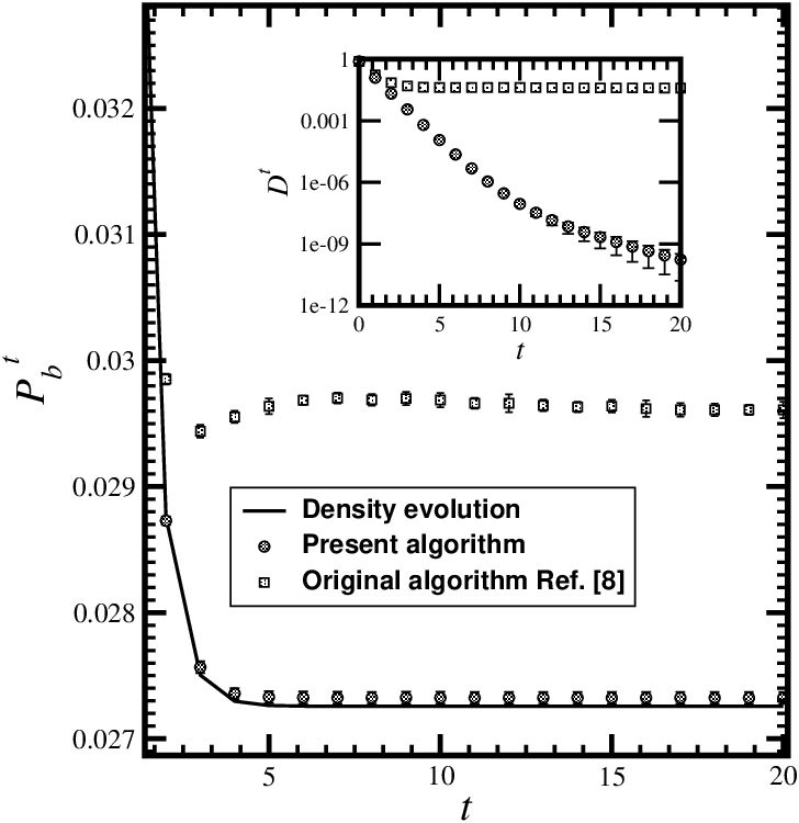
Figure 2: Error probability of the inferred solution evolving in time. The system load β=0.25\beta=0.25, true noise level σ02=0.25\sigma_{0}^{2}=0.25 and estimated noise σ2=0.01\sigma^{2}=0.01. Squares represent results of the original algorithm Kabashima_CDMA, solid line the dynamics obtained from our equations; circles represent results obtained from the suggested practical algorithm. Variances are smaller than the symbol size. In the inset, DtD^{t}, a measure of convergence in the obtained solutions, as a function of time; symbols are as in the main figure.

The inference algorithm requires an iterative update of Eqs.(18,19,17) and converges to a reliable estimate of the signal, with no need for an accurate prior information of the noise level. The computational complexity of the algorithm is of 𝒪⁡(K2){\cal O}(K^{2}).

To test the performance of our algorithm we carried out a set of experiments of CDMA signal detection problem under typical conditions. Error probability of the inferred signals has been calculated for a system load of β=0.25\beta\!=\!0.25, where the true noise level is σ02=0.25\sigma_{0}^{2}\!=\!0.25 and the estimated noise is σ2=0.01\sigma^{2}\!=\!0.01, as shown in Figure 2. The solid line represents the expected theoretical results (density evolution), knowing the exact values of σ02\sigma_{0}^{2} and σ2\sigma^{2}, while circles represent simulation results obtained via the suggested practical algorithm, where no such knowledge is assumed. The results presented are based on 10510^{5} trials per point and a system size N=2000N\!=\!2000 and are superior to those obtained using the original algorithm Kabashima_CDMA.

Another performance measure one should consider is

Dt≡1K​(𝐦t−𝐦t−1)⋅(𝐦t−𝐦t−1),D^{t}\equiv\frac{1}{K}\left(\mathbf{m}^{t}-\mathbf{m}^{t-1}\right)\cdot\left(\mathbf{m}^{t}-\mathbf{m}^{t-1}\right),

that provides an indication to the stability of the solutions obtained. In the inset of Figure 2 we see that results obtained from our algorithm show convergence to a reliable solution in stark contrast to the original algorithm Kabashima_CDMA. The physical interpretation of the difference between the two results is assumed to be related to a replica symmetry breaking phenomena.

In summary, we present a new algorithm for using belief propagation in densely connected systems that enables one to obtain reliable solutions even when the solution space is fragmented. It represents an extension to existing algorithms of that type which is reminiscent to the extension of BP to SP. The algorithm has been tested on the signal detection problem in CDMA and has provided superior results to other existing algorithms Kabashima_CDMA; Kabashima_new. Further research is required to fully determine the potential of the new algorithm.

Support from the EU FP-6 EVERGROW IP is gratefully acknowledged.

References

  • (1) J. Pearl, Probabilistic Reasoning in Intelligent Systems, Morgan Kaufmann Publishers, San Francisco, CA (1988)
  • (2) F.V. Jensen, An Introduction to Bayesian Networks, UCL Press, London (1996)
  • (3) D.J.C. MacKay, Information Theory, Inference and Learning Algorithms, Cambridge University Press (2003)
  • (4) Y. Weiss Neural Computation 12 1 (2000)
  • (5) M. Opper and D. Saad, Advanced Mean Field Methods: Theory and Practice, MIT Press, Cambridge, MA 2001
  • (6) Y. Kabashima, D. Saad, Europhys. Lett. 44 668 (1998)
  • (7) J.S. Yedidia, W.T. Freeman and Y. Weiss, in Advances in Neural Information Processing Systems 13 698 (2000)
  • (8) Y. Kabashima, J. Phys. A 36 11111 (2003)
  • (9) M. Mézard, G. Parisi and M.A Virasoro, Spin Glass Theory and Beyond, World Scientific, Singapore (1987)
  • (10) H. Nishimori, Statistical Physics of Spin Glasses and Information Processing, Oxford University Press UK (2001)
  • (11) M. Mézard, G. Parisi and R. Zecchina, Science 297 812 (2002)
  • (12) M. Mézard and R. Zecchina Phys. Rev. E 66 056126 (2002)
  • (13) S. Verdú, Multiuser Detection, Cambridge University Press UK (1998)
  • (14) D. Saad and M. Rattray, Phys. Rev. Lett. 79 2578 (1997)
  • (15) In preparing the manuscript we have found that a similar activity is being carried out by Yoshiyuki Kabashima at TITECH. However, in the absence of details we cannot comment on his approach.