Systematic Method for Path-Complete White Box Testing
Abstract
A systematic, language-independent method of finding a minimal set of paths covering the code of a sequential program is proposed for application in White Box testing. Execution of all paths from the set ensures also statement coverage. Execution fault marks problematic areas of the code. The method starts from a UML activity diagram of a program. The diagram is transformed into a directed graph: graph’s nodes substitute decision and action points; graph’s directed edges substitute action arrows.
The number of independent paths equals easy-to-compute cyclomatic complexity of the graph. Association of a vector to each path creates a path vector space. Independence of the paths is equivalent to linear independence of the vectors. It is sufficient to test any base of the path space to complete the procedure. An effective algorithm for choosing the base paths is presented.
Key words: White Box testing, open code test, independent paths, UML applications, test completeness, graph theory applications.
1 Introduction
For many years there have been theoretical studies of software, in which the code structure is represented as a graph. In particular, McCabe [1] introduced cyclomatic complexity, known from graph theory, as a measure of complexity of software. It is also known [1] that cyclomatic complexity describes the number of independent paths through the code. Therefore, cyclomatic complexity might be used in planning White Box software testing. However, the practical side of this direction has not been explored. There are some discouraging results from graph theory telling that general problems of finding independent paths are NP-complete (e.g. [6] and references therein). On the other hand, these complexity results are obtained for graphs not necessary representing software. They are too general for the software testing purposes. Software structure imposes important constraints on the graph’s structure and makes problem of finding paths in such graph manageable. For example, every sequential software has two characteristic nodes, the starting point and the finishing point, and all the paths have to include these two nodes. For convenience the starting point of a program is called begin node, whereas the finishing point is called end node, without any assumption about the programming language, in which software is written.
In any graph corresponding to sequential code there is always a path, which is the shortest (actually there may be more than one such path, but one of them can be always chosen). In the paper this path is called backbone path. The whole structure of the code is built around this path. The graph structure of a software code is relatively simple, usually with just a few repeating constructs. As a result, it is possible to create an algorithm, which allows for finding a set of independent paths through arbitrary sequential code in a relatively easy way. This paper presents new, more efficient approach to finding independent paths and planning White Box testing.
There are many definitions of White Box software testing and its completeness. Test completeness means that a predefined scope of testing is exhausted. It is always a matter of choice which scope of testing is needed, as no such thing as a perfect test, disclosing every possible problem, exists. In this paper White Box testing is called complete (path-complete) when software is checked against major design flaws, the flaws are removed, and then each line of the code is successfully executed at least once during the test. In the literature (e.g. [2]) the latter property is called statement coverage. Statement coverage is usually considered as a minimum coverage requirement. However, even some professional testers do not think it is necessary to achieve this level of testing completeness. Half-jokingly, Beizer [2] calls such approach “criminal”. The level of completeness achieved within the proposed method is actually higher than statement coverage. Checking against the major design flaws is in fact a prerequisite in this method. Only software free of them can be properly tested.
The question how to test a known path has been already discussed in [3] resulting in a patented software performing such tests [5], thus, it is not covered in this paper. From the paper by Gunter and Peled [4], and from private communication with one of them (Gunter) it seems that the tool has some limitations, in particular with respect to data types that might be entered. For the purpose of this paper it is assumed that for any valid path through a program it is possible to test it. Not only does the method presented in this paper minimize a number of test paths needed to cover a program code, but it also helps in identifying as short test paths as reasonably achievable. Nevertheless, sometimes, when dealing with a complicated real life software, one or more of the initially identified test paths may be in fact very difficult or just impractical to test. There is no need to spend excessive time on dealing with such cases. The unusually difficult paths can be substituted by others, according to the rules discussed in section 7.
The paper is outlined as follows. The development of a method for systematic White Box testing is discussed in the next sections: in section 2 a control flow chart for a program is derived, and checking against major design flaws is discussed; in section 3 a graph description of the program is introduced, which enables calculation of the number of independent paths in the program; in section 4 a vector space of paths is defined and a simple method for checking path independence is presented; in section 5 a practical method for finding simplest independent paths is shown. In section 6 an algorithm for test-planning is presented, and in section 7 practical applications of a path vector space in the test-planning are shown. Finally, in section 8 a summary of the work and an overview of further research and possible applications are given.
2 Activity diagrams of a program and detection of major design flaws
The first step of the proposed method is creation of a flow chart. Any type of a flow chart can be used, if needed. In order to standardize the approach and make it programming language independent, a UML activity diagram is used in this paper. For many programmers constructing an activity diagram is a routine step in software design. In case a program is written without constructing an activity diagram at the design stage, it can be reconstructed from the software code, as for each sequential program a UML activity diagram can be constructed. Lines of the code are assigned to decision or action points of its activity diagram.
Before proceeding further, it is necessary to check the code against major design flaws. Major design flaws include: parts of a code that can never be executed, values that are calculated but never used, redundant execution of the same piece of a code, or any overcomplicated code, which can be easily refactored.
Horrible loops described in [2], i.e. multiple loops, which are neither nested nor consecutive, are clearly identified by an activity diagram. Examples of horrible loops include intersecting loops, cross-connected loops, jumps into and out of loops, and hidden loops. Such constructions should be removed from a program before further testing.
Procedures with multiple entrances and/or exits, which appear in some old programs, for instance written in Fortran, may cause another design problem. They are known also as ill-formed procedures and their modification is generally advised [2]. In case of multiple entrances an additional, external entry point should be added. It is a decision point directing control flow to the appropriate initial entry point. Similarly, in case of multiple exits an external exit should be added. All the initial exits would be then directed to it. Such a modification of an ill-formed procedure is needed for applying the next part of the method discussed here.
Pachinko code is an example of extreme control flow: a program that modifies its own instructions. There is no known method for testing it [2], hence the only way is to redesign such a program. Only software free of these flaws may be properly tested.
Spaghetti code, in which control structure is tangled due to multiple go-to jumps and other branching constructs, is not a mark of good contemporary design. Nevertheless, if it is free of horrible loops, it still might be tested by the method proposed further. On the other hand, redesigning spaghetti code is strongly suggested by software designers that can be achieved easily using activity diagram.
3 Graph representation of a program, independent paths
After creating an activity diagram for a code and removing any design flaws found, the next step is to create a directed graph representing the control flow in the code. The directed graph is built from the UML activity diagram in the following way: graph nodes are substituted for all the decision and action points, directed edges of the graph are substituted for the action arrows. Such a graph contains a single input node (begin) and a single output node (end). A virtual edge from begin node of the graph to end node is used to close the directed graph. This way the graph becomes strongly connected.
Definition. A strongly connected graph is a graph, whose any two nodes are connected by a path, which is a sequence of consecutive directed edges.
From the graph topology point of view, independent paths closed by the same virtual edge can be understood as cycles constituting the first homology space for the graph supplemented by the virtual edge. Hence cyclomatic complexity, which is of basic importance for this work, is equal to the first Betti number for the graph (e.g. [7]).
The number of independent paths in the whole program as well as the number of independent paths inside any module or inside a complex loop can be established just by counting the number of edges and nodes of the corresponding graph. It is one of the measures of software complexity. It has an advantage over language-dependent or even programming-style-dependent code measures like the number of lines, because it is related to logical structure of a program (decisions, loops).
For a strongly connected graph the number of independent paths is equal to the cyclomatic complexity number of the graph. The complexity number, , of a graph is defined as
| (1) |
where is the number of edges in the graph, and is the number of its nodes. A virtual edge should be added to make the obtained graph strongly connected. Therefore, the number of edges is increased by one, and (1) becomes .
Transition from an activity diagram to a directed graph preserves paths. It is desirable to use independent paths in software testing for computational efficiency. In the next section of the paper, a vector representation of the paths is introduced. Path independence can be checked easily using this vector description.
Definition. A path is independent from a set of other paths if for any path , , there exists a part of a code executed by the path such that it is never executed by the path .
Loops and jumps are special constructs in software, that is why their representation should be discussed in more detail. In case of consecutive loops, each of them is treated separately; nested loops are treated as subgraphs. At this stage of the method the code is expected to be already free of all other multi-loop constructions, like intertwining loops or hidden loops [2].
In the loops of the most common type a condition is evaluated before execution of the loop. A typical example is for construct. According to the convention introduced earlier, it is sufficient to traverse each edge of a graph once to reach completeness of the testing. In other words it is sufficient to traverse a loop once, if it does not have internal decision points or internal loops. A subgraph of a loop with internal structure can be considered separately from the main graph such that a condition-checking vertex becomes both begin and end nodes. The number of independent paths needed to test such a loop is determined by structure of this subgraph.
There is also another type of loops, in which the condition is evaluated at the bottom of the loop, for instance do-while construct. A body of such a loop is executed once before the condition is ever checked. After that the loop execution is done similarly to for loop. In other words, a do-while loop can be represented via while loop (which is equivalent to for loop) as follows:
This formalism shows that only one type of loops is needed for a graph representation.
A construct called go-to jump is not recommended in modern programming. This construct distorts a coding block and hence eliminates any visual cues about the flow of control. Even though it can be avoided, some programmers still use go-to. Therefore, in order for the method to be complete it should be able to handle this construct as well. In case of a forward go-to jump, it can be represented as an additional edge between go-to and its label. Otherwise, if the jump is backward, it can be represented similarly to do-while loop discussed above.
There is yet another issue to consider: is it sufficient to traverse a loop only once during testing? For finding paths, only one execution of a simple loop (a loop without internal loops or decision points) is assumed. The problem of a number of executions of a loop is not handled by presented method, since finding the paths is the focus of this paper, not their testing. Once the loop path is established, it can be tested as needed. Usually it is much easier to do so after the path structure for the whole program is identified.

Figure 1 shows an example of a graph constructed from the software for object reconstruction from X-ray images.
4 Vector representation of paths
In order to check path independence a vector is assigned to each possible path. The number of elements of each vector equals the number of edges in the graph. Note that edges have to be ordered, however the order can be arbitrary. Each element of the vector corresponding to a particular edge indicates whether the edge belongs to the path or not. The element is equal to 1 if the edge belongs to the corresponding path or 0 otherwise.
Since elements of the vector can only be 0 or 1, the vector space of paths is defined over ZZ2 (the field of integers modulo 2). Linearly independent vectors represent independent paths, which enables checking paths’ independence by showing linear independence of the vectors representing them. Even though the vectors’ length is large, their elements are only zeros or ones. Moreover all calculations are done modulo 2 that is why the computation is still simple.
The dimension of a path vector space is equal to the number of independent paths in a graph, i.e. to cyclomatic complexity of the graph. Therefore, any set of C vectors representing independent paths forms a base in this vector space.
It is sufficient to restrict testing only to the base paths in order to guarantee that all the nodes are visited, i.e. to achieve statement coverage [2]. In fact with this method a path coverage is achieved, which is more than just statement coverage. A choice of the base paths is obviously not unique. For the practical reasons it is very important to choose the base in a convenient way. A method for choosing the base is discussed below. Checking for linear independence of appropriate vectors is sufficient for showing independence of corresponding paths.
This concludes the presentation of a theoretical basis of a general procedure. The following section of the paper introduces a method for effective choice of the base paths. This method is powerful enough to handle relatively complex software. It is oriented towards choosing a set of the simplest independent paths among different possibilities.
5 Method for effective selection of the base paths
5.1 Backbone path
Each path in a graph constructed accordingly to the rules described above connects begin and end nodes. Recall that a path that contains the minimum number of edges is called a backbone path. It is possible and, in fact, not uncommon that more than one path with the minimum number of nodes exists; any one of them can be chosen to be a backbone path. The only fact important for further consideration is that for any sequential software it is always possible to choose a backbone path. Choosing the simplest possible path is not a strict requirement, however it simplifies all the next steps of the method.
5.2 Loops
Loops are special components of a graph. Any graph can be represented as a merge of its loopless part and loop-graphs. A loopless part of a graph is obtained by removing all its loops, whereas a loop-graph is a subgraph, which represents a loop of arbitrary complexity (see figure 2).

A loop can originate inside another loop or block (loops (h) and (bef) of figure 2) or on a backbone path (loop (o) of figure 2). In this construction nested loops are represented by the outermost loop. If a loop originates on a backbone path, its extended loop-graph consists of the loop added to the backbone (path xn(o)py for loop (o); parentheses indicate looping inside of a path). Otherwise, if a loop originates outside of a backbone path (inside of a block) an extended loop-graph consists of the loop with the shortest path between begin and end of a block added to a part of the backbone path outside this block (path xa(bef)gilmnpy for loop (bef)).
After this reduction, the vector space of all possible paths can be represented as a direct sum of the space for the loopless part of the graph and each of the spaces for extended loop-graphs described above. Stated another way, if is a vector space of the loopless part, is a vector space of paths of the extended loop-graph, where and is the number of loops, then vector space of paths of the graph is
A simple loop, which does not have nested loops or conditionals, can be tested by executing a single path passing through the loop. On the other hand, a complex loop can be considered separately, since it is represented by a strongly connected subgraph with single begin and end nodes (it is strongly connected since a virtual edge from end to begin is assumed). This method can be applied recursively on this subgraph to obtain its independent paths.
5.3 Modularity of a program
In this subsection loopless part of a graph is considered. It is common that graphs of sequential programs, especially long ones, contain cut-vertices.
Definition. A cut-vertex of a graph, also known as an articulation point, is a node whose removal disconnects the graph.
This definition implies that every path in a software graph passes through every cut-vertex of the graph.
Definition. A part of a graph between two cut-vertices is called a module in software development and a block in graph theory.
A block can also be closed by a virtual edge, hence the number of independent paths in a block can be calculated the same way as for the whole graph.
Each block can be considered as a subgraph with its own cyclomatic complexity number and its own set of paths. A section of a backbone path belonging to the block should be identified as one of the base paths in this block. When a base of a block path space is established, all the paths are complemented by segments of the backbone path outside of the block (see subsection 5.2 for details).
A complex block can be divided into two or more parallel parts. A path space of a block is a sum of path spaces of all the parts. In case any part has a cut-vertex(ices) it can be divided into its own sub-blocks. Division into smaller and smaller sub-blocks can be repeated until the smallest units are reached, sub-blocks of which are trivial.
Some remarks about how to build a base of the path space for the whole graph from bases of path spaces for its blocks and loop-graphs should be made. Every block shares a backbone path with other blocks, hence one of the base paths of each module is a segment of the backbone path. Any two base paths with non-backbone segments included in different blocks are independent.
Merging all bases of block paths and loop paths can serve as a base of the graph. A merge operation here is a set union, therefore, a backbone path appearing in the base of each block is included only once.
Not only does this method make the process of finding the base paths relatively simple, but it also constructs paths which are generally shorter than their possible alternatives. In addition there are several other advantages of the method.
One of them is better localization of the problem in the code than the one provided by traditional testing methods. In case one of the base paths fails the test, the failure can be localized to the part of the code corresponding to this path, and frequently even to a part of this path in a particular module.
It is also important that a recursive approach allows for applying the method effectively to a sequential program of practically any complexity.
6 Path-choosing algorithm
In this section an effective algorithm for path finding is proposed. It can be applied to the whole program as well as to its submodules. The method, called TEST, is presented in a pseudo-code.
TEST(C):
INPUT: software code C.
OUTPUT: set P of all independent paths.
BEGIN
1. A=get_activity_diagram(C);
2. A=purify(A);
3. G=get_graph(A);
4. n=get_number_indep_paths(G);
5. P=compute_paths(G);
END
In the first step of the algorithm a UML activity diagram of the software denoted as C is prepared. Function purify, which is called afterwards, eliminates design flaws, if any, and optimizes the software design, if applicable. After that the activity diagram is translated into a directed graph by calling function get_graph. Finally, the number of independent paths (read cyclomatic complexity) through the connected graph obtained in the previous step is calculated and function compute_paths is called. The latter function is the actual algorithm for finding independent paths of a strongly connected graph. Its pseudo-code is given below.
compute_paths(C):
INPUT: directed, strongly connected graph G.
OUTPUT: set P of all independent paths of graph G.
BEGIN
1. P=;
2. loop
2.1. Mi=get_block(G);
2.2. if(Mi==G)
2.2.1. Pi=count(Mi);
2.3. else
2.3.1. Pi=compute_paths(Mi);
2.4. P=combine_paths(P,Pi);
3. loop until(no sub-blocks left);
END
Function compute_paths is a recursion: it recursively computes independent paths of each sub-block of the given graph and then combines these sets together. Function combine_paths, which performs such combining, is given below. Note also that the base case of the recursion is computed by count, which is a simple enumeration of independent paths in the trivial sub-block.
combine_paths(P1,P2):
INPUT: two sets of independent paths: P1 and P2.
OUTPUT: set P of independent paths created from P1 and P2.
BEGIN
1. b1=get_backbone(P1);
2. b2=get_backbone(P2);
3. for(each path a1P1: a1b1)
3.1. P=add(P,a1b2);
4. for(each path a2P2: a2b2)
4.1. P=add(P,b1a2);
END
The idea of function combine_paths is to append each path from P1 with a backbone path of P2 creating a subset of paths. Similarly, each path from P2 is appended to a backbone path of P1 creating another subset of paths, which is then merged with the first one. Operation ”” in the program above is an append of two paths. Note that the paths order during the append is important. Function add in the program is an inclusion of a given path into a path set.
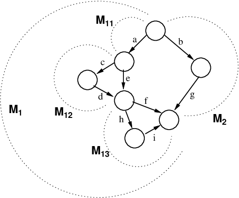
As an example function compute_paths is applied to a graph in figure 3. The graph is divided into two blocks: M1 and M2, and the function is recursively called on each block. In case of the block M1, it is further divided into M11, M12, and M13. Block M11 cannot be divided anymore, hence P11=count(M11)={a}. A recursive call of compute_paths on M12 returns P12={e,cd} which needs to be combined with P=P11. Combined P trivially equals to {ae,acd}. Similarly, P13=compute_paths(M13)={f,hi}. While combining P13 with current P, the backbone of each set is identified: f and ae correspondingly. The combination of two sets is P={aef,aehi,acdf}. Consequently, the final set of independent paths for the graph from figure 3 is P={aef,aehi,acdf,bg}.
This algorithm finds the minimal number of paths and constructs paths needed to be tested for a complete (in the sense of path-completeness) White Box testing. Since each path diverts from the backbone path inside of only one module loop, it might be relatively easy to localize the problem to a particular module/loop when a path fails a test. Tracing where the path diverts from other paths inside the same module can localize the problem area even further.
7 Applications of vector space in path finding
Vectors can be assigned to each path in the way described before. Checking a number of the paths established using the path-finding algorithm as well as linear independence of their vectors independently verifies that test paths are established correctly. In case of any possible mistake checking the number of independent paths contributed by each of the blocks and loops quickly localizes the problem inside one of them.
A vector space of all paths through the graph , can be represented as a simple sum of a vector space of paths for loopless part of the graph and all of the extended loop graphs , where is the number of extended loop graphs:
| (2) |
All blocks, on the other hand, share a backbone path, which is one of the base paths for each of them. This is why each block contributes one path less than the dimension of its paths vector space, and the backbone path is counted once:
| (3) |
where , , and represent complexity numbers of the whole graph (equals ), a loopless block, and an extended loop graph correspondingly.
An experienced tester dealing with a relatively simple graph (a module, a loop) may not need to apply the algorithm at all, but use the intuition to guess an appropriate number of paths and check linear independence of their vectors. In cases when it is applicable, such an approach simplifies the method even more.
It may happen that some of the initially identified base paths are difficult or practically impossible to test. In this situation a new base is established by supplementing the to-be-tested base paths with a set of paths, which are different from rejected ones, but independent from the other base paths. Substituting two or more base paths by more convenient for testing paths may be a time saving strategy, while preserving test-completeness.
8 Conclusion
In this paper, using graph theory, an effective algorithm for finding sets of independent paths in sequential software is found. In addition, an efficient method for independence checking based on linear algebra is given. The method finds a base in the set of independent paths, and shows that the resulting set of paths constitutes a base. Testing any base paths completes White Box testing. Therefore, proposed algorithm allows for planning White Box software testing in a systematic way, and for performing such testing in a complete way in the sense of path completeness.
There are two possible directions for the future work. The first direction is to implement the White Box testing method described in the paper. The second is to generalize the method to handle parallel programs. A UML activity diagram can be constructed for parallel software, which in turn can be transformed into a directed graph similarly to the sequential case. The main challenge is that in general parallel software has to be tested not only for execution of every possible path but also for synchronization between the executions of different parts of the code.
9 Acknowledgements
The research was connected to work on an X-ray image recognition project. The authors are grateful to members of the Data Driven Modelling and Analysis team for their help, particularly to Tom Asaki for his hospitality, discussions and enthusiasm. The help of Collin Powell for providing the ProtoReX MatLab code, on which initial ideas were tested, is acknowledged.
The authors are thankful to David Aubrey for extensive discussions and many practical suggestions about software testing.
Many thanks to Josef Przytycki for discussions and checking the graph-theoretical basis of the method.
References
- [1] McCabe T. Complexity measure, IEEE Transacions on Software Engineering, 1976; 2(4): 308–320.
- [2] Beizer B. Software Testing. International Thompson Computer Press, 1990.
- [3] Gunter E., Peled D. Path exploration tool, Proc. of 5th International Conference on Tools and Algorithms for Construction and Analysis of Systems, LNCS, 1999; 1579: 405–419.
- [4] Gunter E., Peled D. Unit Checking: Symbolic Model Checking for a Unit of Code, International Symposium on Verification (Theory & Practice), LNSC, 2004; 2772: 548–568.
- [5] Gunter E., Peled D., United States Patent: 6,408.430; Interactive software testing system and method, 2002.
- [6] Erlebach T., Vukadinović D. New Results for Path Problems in Generalized Stars, Complete Graphs, and Brick Wall Graphs, Proc. of the 13th International Symposium on Fundamentals of Computation Theory, LNCS, 2001; 2138: 483–494.
- [7] Duke R. The genus, regional number, and Betti number of a graph, Canadian Journal of Mathematics, 1966; 18: 817–822.