On the Scalability of Cooperative Time Synchronization in Pulse-Connected Networks Thanks: The authors are with the School of Electrical and Computer Engineering, Cornell University, Ithaca, NY. URL: http://cn.ece.cornell.edu/. Work supported by the National Science Foundation, under awards CCR-0238271 (CAREER), CCR-0330059, and ANR-0325556.
Abstract
The problem of time synchronization in dense wireless networks is considered. Well established synchronization techniques suffer from an inherent scalability problem in that synchronization errors grow with an increasing number of hops across the network. In this work, a model for communication in wireless networks is first developed, and then the model is used to define a new time synchronization mechanism. A salient feature of the proposed method is that, in the regime of asymptotically dense networks, it can average out all random errors and maintain global synchronization in the sense that all nodes in the multi-hop network can see identical timing signals. This is irrespective of the distance separating any two nodes.
Index Terms:
Cooperation in networks, large network asymptotics, relay networks, scalability, sensor networks, time synchronization, wireless communications.I Introduction
I-A Time Synchronization in Large Distributed Systems
The problem of time synchronization in large distributed systems consists of giving all the physically disjoint elements of the system a common time scale on which to operate. This common time scale is usually achieved by periodically synchronizing the clock at each element to a reference time source, so that the local time seen by each element of the system is approximately the same. Time synchronization plays an important role in many systems in that it allows the entire system to cooperate and function as a cohesive group.
Time synchronization is an old problem [26], but the question of scalability is not. Recent advances in sensor networks show a clear trend towards the development of large scale networks with high node density. For example, a hardware simulation-and-deployment platform for wireless sensor networks capable of simulating networks with on the order of 100,000 nodes was recently developed [24]. As well, for many years the Smart Dust project sought to build cubic-millimeter motes for a wide range of applications [43]. Also, there is work in progress on the drastic miniaturization of power sources [27]. These developments (and many others) indicate that large scale, high density networks are on the horizon.
Large scale, high density networks have applications in a variety of situations. Consider, for example, the military application of sniper localization. Large numbers of wireless nodes can be deployed to find the shooter location as well as the trajectory of the projectile [1]. Since the effective range of a long-range sniper rifle can be nearly km, in order to fully track the trajectory of the projectile it may be essential that our deployed network be tightly synchronized over distances of a few kilometers. Another example might be the implementation of a distributed radio for communication. In extracting information from a deployed sensor network, it may be beneficial for the nodes to cooperatively transmit information to a far away receiver [6, 7, 20]. Such an application would require that nodes across the network be well synchronized. As a result, a need for the synchronization of large distributed systems is very real and one that requires careful study to understand the fundamental performance limits on synchronization.
I-B Approaches to Synchronization and the Limitations
The synchronization of large networks has been studied in fields ranging from biology to electrical engineering. The study of synchronous behavior has generally taken one of two approaches. The first approach is to consider synchronization as an emergent behavior in complex networks of oscillators. In that work, models are developed to describe natural phenomena and synchronization emerges from these models. The second approach is to develop and analyze algorithms that synchronize engineering networks. Nodes are programmed with algorithms that estimate clock skew and clock offset to achieve network synchronization. However, both of these approaches have significant limitations.
I-B1 The Emergence of Synchronous Behavior
Emergent synchronization properties in large populations has been the object of intense study in the applied mathematics ([30, 41]), physics ([3, 4, 5, 9, 12, 14, 16, 25]), and neural networks ([21, 37]) literature. These studies were motivated by a number of examples observed in nature:
- •
In certain parts of south-east Asia, thousands of male fireflies congregate in trees and flash in synchrony at night [2].
- •
Pacemaker cells of the heart, which on average cause 80 contractions a minute during a person’s lifetime [22].
- •
The insulin-secreting cells of the pancreas [35].
For further information and examples, see [32, 40, 31, 42], and the references therein.
A number of models have been proposed to explain the emergence of synchrony, but perhaps one of the most successful and well known is the model of pulse-coupled oscillators by Mirollo and Strogatz [32], based on dynamical systems theory. Consider a function that is smooth, monotone increasing, concave down (i.e., and ), and is such that and . Consider also a phase variable such that , where is the period of a cycle. Then, each element in a group of oscillators is described by a state variable and a phase variable as follows:
- •
In isolation, .
- •
If then , and if then .
- •
When for any of the ’s and some time , then for all other ,
where denotes an infinitesimal amount of time after . That is, oscillator reaching the end of a cycle causes the state of all other oscillators to increase by the amount , and the phase variable to change accordingly.
The state variable can be thought of as a voltage. Charge is accumulated over time according to the nonlinearity and it discharges once it reaches full charge, resetting the charging process. Upon discharging, it causes all other charges to increase by a fixed amount of , up to the discharge point. For this model, it is proved in [32] that for all and for almost all initial conditions, the system eventually becomes synchronized.
For the network to converge into a synchronous state, one key assumption is that the behavior of every single oscillator is governed by the same function . This means that all oscillators must have the same frequency. From the literature, it appears that this requirement is nearly always needed. As far as we are aware, for a fully synchronous behavior to emerge, the oscillators need to have the same, or nearly the same, oscillation frequencies.
The need for nearly identical oscillators presents a significant limitation for emergent synchronization. This emergence of synchrony is clearly desirable and it has been considered for communication and sensor networks in [17, 18, 28]. However, whether or not these techniques can be adapted to synchronize networks with nodes that have arbitrary oscillator frequencies (clock skew) is still unclear. Thus, in order to overcome this limitation and find techniques capable of synchronizing a more general class of networks, we turn to algorithms designed to estimate certain unknown parameters such as clock skew.
I-B2 Estimation of Synchronization Parameters and the Scalability Problem
There have been many synchronization techniques proposed for use in sensor networks. These algorithms generally allow each node to estimate its clock skew and clock offset relative to the reference clock. Reference Broadcast Synchronization (RBS) [8] eliminates transmitter side uncertainties by having a transmitter broadcast reference packets to the surrounding nodes. The receiving nodes then synchronize to each other using the arrival of the reference packets as synchronization events. Tiny-Sync/Mini-Sync [36] and the Timing-sync Protocol for Sensor Networks (TPSN) [11] organize the network into a hierarchial structure and the nodes are synchronized using pair-wise synchronization. In lightweight tree-based synchronization (LTS) [13], pair-wise synchronization is also employed but the goal of LTS is to reduce communication and computation requirements by taking advantage of relaxed accuracy constraints. The Flooding Time Synchronization Protocol (FTSP) [29] achieves one-hop synchronization by having a root node broadcast timing information to surrounding nodes. These surrounding nodes then proceed to broadcast their synchronized timing information to nodes beyond the broadcast domain of the root node. This process can continue for multi-hop networks.
The problem with each of these traditional synchronization techniques is that synchronization error will increase with each hop. Since each node is estimating certain synchronization parameters, i.e. clock skew, there will be inherent errors in the estimate. As a result, a node multiple hops away from the node with the reference clock will be estimating its parameters from intermediate nodes that already have estimation errors. Therefore, this introduces a fundamental scalability problem: as the number of hops across the network grows, the synchronization error across the network will also grow.
Current trends in network technology are clearly moving us in the direction of large, multi-hop networks. First, sensors are decreasing in size and this size decrease will most likely be accompanied by a decrease in communication range. Thus, more hops will be required to traverse a network deployed over a given area. Second, as we deploy networks over larger and larger areas, then for a given communication range, the number hops across the network will also increase. In either case, the increased number of hops required to communicate across the network will increase synchronization error. Therefore, it is essential that we develop techniques than can mitigate the accumulation of synchronization error over multiple hops.
I-C Spatial Averaging and Synchronization
I-C1 Cooperation through Spatial Averaging
To decrease the error increase in each hop, we need to decrease the estimation error. There are two primary ways of achieving this. First, each node can increase the amount of timing information it obtains from neighboring nodes. For example, from a received timing packet, the node may be able to construct a data point telling it the approximate time at the reference clock and the corresponding time at its local clock. Using a collection of these data points, the node can estimate clock skew and clock offset. So instead of using, say, five packets with timing information, a node can wait for ten packets. More data points will generally give better estimates. The drawback to such an approach is the increase in the number of packet exchanges.
The second way in which to reduce estimation error is to increase the quality of each data point obtained by the nodes. This can be achieved through improving packet exchange algorithms and time stamping techniques. However, we believe that there is one fundamentally new approach to improving data point quality that has not be carefully studied. This is to use spatial averaging to improve the quality of each data point.
The motivation for this approach is very simple. Assume that each node has many neighbors. If all nodes in the network are to be synchronized, then the neighbors of any given node will also have synchronization information. Is it possible to simultaneously use information from all the neighbors to improve the quality of a timing observation made by a node? Furthermore, it would seem to make sense that with more neighbors, hence more available timing information, the quality of the constructed data point should improve. If this is indeed the case, then achieving synchronization through the use of spatial averaging will provide a fundamentally new trade-off in improving synchronization performance. Network designers would simply be able to increase the number and density of nodes to obtain better network synchronization. The study of cooperative time synchronization using spatial averaging is the focus of this work.
I-C2 Model and Technique
To obtain a model for developing cooperative synchronization in large wireless networks, we begin by looking at the signals observed by a node in a network with nodes uniformly deployed over a fixed finite area. To start, we assume propagation delay to negligible (the general case is considered in Section V). All nodes transmit a pulse and a node will see a signal which is the superposition of all these pulses,
In this expression, is the basic pulse transmitted by each node (assumed to be the same for all nodes). is the ideal pulse transmit time, but since we assume imperfect time synchronization among the nodes we have modelling random errors in the pulse transmission time. models the amplitude loss in the signal transmitted by the th node. is the maximum magnitude transmitted by a node. We scale each node’s transmission by so that as the network density grows, the total power radiated does not grow unbounded. This model thus describes the received signal seen at a node for a network with nodes and this holds for any . Increasing will have two effects: (a) node density will increase since the network area is fixed and (b) node signal transmission magnitude will decrease due to the scaling. Therefore, by increasing this model allows us to study the scalability of networks as node density grows and node size decreases.
Given that these are the signals observed at each node, we ask: is it possible for to encode a time synchronization signal that will enable all nodes in the network to synchronize their clocks with bounded error, as ? The answer is yes, and the key to proving all our results is the law of large numbers.
Our key idea is the following. If all nodes were able to determine when time (in the reference time) arrives, then by transmitting at time , the signal observed at any node would be , which is a suitably scaled version of centered at . In reality however, there will be some error in the determination of , which we account for by allowing for a node-dependent random error . But, if the distribution of satisfies certain conditions, then the effects of that timing error can be averaged out. A pictorial representation of why this should be the case is shown in Fig. 1.


Therefore, intuitively we can see how the technique of cooperative time synchronization using spatial averaging can average out the inherent timing errors in each node. Even though there is randomness and uncertainty in each node’s estimates, by using cooperation among a large number of nodes it is possible to recover deterministic parameters from the resulting aggregate waveform (such as the location of certain zero-crossings) in the limit as node density grows unbounded. Thus more nodes will give us better estimates. This is because the random waveform converges to a deterministic one as more and more nodes cooperatively generate an aggregate waveform. At the same time, the average power required by each node will decrease since smaller nodes send smaller signals. Therefore, by programming suitable dynamics into the nodes, in this paper we show how it is possible to generate an aggregate output signal with equispaced zero-crossings in the limit of asymptotically dense networks. Thus, the detection of these zero-crossings plays the same role as that of an externally generated time reference signal based on which all nodes can synchronize.
We develop this synchronization technique in three main steps. One, we set up the model for . Two, we specify characteristics of the model (i.e. the distribution of ) that allow us to prove desirable properties of the aggregate waveform (such as a center zero-crossing at ). Three, we develop the estimators needed for our synchronization technique and show that the estimators give us the desired characteristics.
I-D Main Contributions and Organization of the Paper
The main contributions presented in this paper are the following;
- •
The definition of a probabilistic model for the study of the time synchronization problem in wireless networks. This model does contain the classical Mirollo-Strogatz model as a special case, but its formulation and the tools used to prove convergence results are of a completely different nature (purely probabilistic, instead of based on the theory of dynamical systems).
- •
Using this model, we provide a rigorous analysis of a new cooperative time synchronization technique that employs spatial averaging and has favorable scaling properties. As the density of nodes increases, synchronization performance improves. In particular, in the limit of infinite density, deterministic parameters for synchronization can be recovered.
- •
We show that cooperative time synchronization works perfectly for negligible propagation delay. When propagation delay is considered, we find that asymmetries at the boundaries reveal some limitations that need to be carefully considered in designing algorithms that take advantage of spatial averaging.
In analyzing the proposed cooperative time synchronization technique, our goal is to show that the proposed technique can average out all random error and provide deterministic parameters for synchronization as node density grows unbounded. This asymptotic result can be viewed as a convergence in scale to synchrony. The result serves as a theoretical foundation for allowing a new trade-off between node density and synchronization performance. In particular, higher node density can yield better synchronization.
The rest of this paper is organized as follows. The general model is presented in Section II. Of particular interest here is Section II-E, where we show how our model contains the model of Mirollo and Strogatz for pulse-coupled oscillators as a special case [32]. In Section III we specialize the general model for our synchronization setup and develop waveform properties that will be used in time synchronization. In Section IV we develop the cooperative time synchronization technique for no propagation delay. We extend the cooperative synchronization ideas to the case of propagation delay in Section V. The paper concludes in Section VI with a detailed discussion on the scalability issue and how the technique proposed in this work lays the theoretical foundation for a general class of cooperative time synchronization techniques that use spatial averaging.
II System Model
II-A Clock Model
We consider a network with nodes uniformly distributed over a fixed finite area. The behavior of each node is governed by a clock that counts up from . The introduction of is important since it provides a consistent timescale for node . By maintaining a table of pulse-arrival times, node can utilize the arrival times of many pulses over an extended period of time.
The clock of one particular node in the network will serve as the reference time and to this clock we wish to synchronize all other nodes. We will call the node with the reference clock node and the clocks of other nodes are defined relative to the clock of node . We never adjust the frequency or offset of the local clock because we wish to maintain a consistent time scale for node .
The clock of node , , will be defined as where . Taking to be the reference clock, we now define the clock of any other arbitrary node , . We define as
| (1) |
where
- •
is an unknown offset between the start times of and .
- •
is a constant and for each , where are finite. This bound on means that the frequency offsets between any two nodes can not be arbitrarily large.
- •
is a stochastic process modeling random timing jitter.
Thus, this model assumes that there is a bounded constant frequency offset between the oscillators of any two nodes as well as some random clock jitter.
It is important to note that node does not have to be special in any way; its clock is simply a reference time on which to define the clocks of the other nodes. This means that our clock model actually describes the relative relationship of all the clocks in the network by using an arbitrary node’s clock as a reference.
II-B Pathloss Only Model
II-B1 A Random Model for Pathloss
From Section I-C2, we see that we are interested in studying the aggregate waveform observed at a node . As a result, we are only concerned with the aggregate signal magnitude and do not care about the particular signal contribution from each surrounding node. With this in mind, we can develop a random model for pathloss that, for dense networks, gives the appropriate aggregate signal magnitude at node . Such a model is ideal for our situation since we are studying asymptotically dense networks.
We start with a general pathloss model , where for all distances , is non-increasing and continuous. is a fraction of the transmitted magnitude seen at distance from the transmitter. For example, if the receiver node is at distance from node , and node transmits a signal of magnitude , then node will hear a signal of magnitude . We derive from a power pathloss model since any pathloss model captures the average received power at a given distance from the transmitter. This average received power is perfect for modelling received signal magnitudes in our problem setup since we are considering asymptotically dense networks. Due to the large number of nodes at any given distance from the receiver, using the average received magnitude at distance as the contribution from each node at that distance will give a good modelling of the amplitude of the aggregate waveform.
The random pathloss variable will be derived from . To understand how and are related, we give an intuitive explanation of the meaning of as follows: the is the fraction of nodes at distances from node such that , where is a small constant. This means that, roughly speaking, for any given scaling factor , is the fraction of received signals with magnitude scaled by approximately , where is the probability density function of . Thus, if we scale the transmit magnitude from every node by an independent , then as the number of nodes, , gets large, node will see signals of approximate magnitude , and this holds for all in the range of . This is because taking a large number of independent samples from a distribution results in a good approximation of the distribution.
Thus, this intuition tells us that scaling the magnitude of the signal transmitted from every node by an independent sample of the random variable gives an aggregate signal at node that is the same magnitude as if we generated the signal using directly. Even though the signals from two nodes at the same distance from a receiver have correlated magnitudes, we do not care about the signal magnitude from any particular node but only that an appropriate number of all possible received signal magnitudes contribute to the aggregate waveform. For a receiving node , we choose therefore to work with the random variable instead of directly with because, for the goals of this paper, doing so has two major advantages: (a) we can obtain desirable limit results by placing very minimal restrictions on the distribution of the ’s (and hence on ) and (b) we can apply tools from probability theory (basically, the strong law of large numbers) to carry out our analysis.
II-B2 Definition of
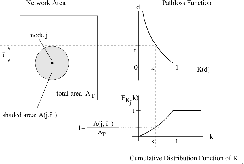
From the above intuition we can define the cumulative distribution function of as
| (2) |
where
- •
is the total area of the network,
- •
is the area of the network contained in a circle of radius centered at node ,
- •
.
From the above discussion we see that the distribution of is only a function of node , the receiving node. We illustrate the relationship among node , , , and in Fig 2. We sometimes write with used to index each node surrounding node . is thus indexing a sequence of independent random variables for fixed . Therefore, for a given , ’s are independent and identically distributed (i.i.d.) with a cumulative distribution function given by (2) for all .
We assume that has the following properties:
- •
is independent from for all , , and .
- •
, , and .
The requirements on the random variable places restrictions on the model . Any function that yields a with the above requirements can be used to model pathloss.
II-C Delay and Pathloss Model
In this section we develop a more complex model to simultaneously model propagation delay and pathloss. This leads to the joint development of the delay random variable and a corresponding pathloss random variable .
II-C1 Correlation Between Delay and Pathloss
Since we want to develop a model for both pathloss and time delay, we start by keeping the pathloss function defined in Section II-B. The general delay model assumes a function that models the time delay as a function of distance. describes the time in terms of that it takes for a signal to propagate a distance . For example, if node and node are distance apart, then a pulse sent by node at time will be seen at node at time . We make the reasonable assumption that is continuous and strictly monotonically increasing for .
As with the pathloss only model, we want to define a delay random variable for each receiving node . Recall that this means that for every node there is a random variable associated with it since, in general, each node will see different delays. There is a correlation between the delay random variable and the pathloss random variable . This correlation arises for two main reasons. First, since in Section II-B we define to be monotonically decreasing and continuous, it is possible for for , . This might be the case for a multi-hop network. In this situation, there will be a set of nodes whose transmissions will never reach node (i.e. infinite delay) even though according to these nodes should contribute a signal with finite delay. Second, a small value would represent a signal from a far away node. As a result, the corresponding value should be large to reflect large delay. Therefore, keeping these two points in mind, we proceed to develop a model for both pathloss and propagation delay.
II-C2 Definition of and
We define the cumulative distribution function of as
| (3) |
where , is a constant, , and
Recall that , defined in Section II-B, is the area of the network contained in a circle of radius centered at node and is the total area of the network. Note that can be infinite.
Using the delay random variable with the cumulative distribution function in (3), we define as
| (4) |
where is the deterministic pathloss function from Section II-B and is the inverse function of the deterministic delay function . Note that exists since is continuous and strictly monotonically increasing on .
II-C3 Intuition Behind and
To understand the distribution of , we need to consider the definition of as well. Recall that a signal arriving with delay is scaled by the pathloss random variable . Let us consider the cumulative distribution in two pieces, and . The case for is trivial. First, for , the probability that takes a value less than or equal to is simply the fraction of the network area around node such that the nodes are at distances with . The intuition is the same as that for the development of in Section II-B. Second, for , the situation is more complex. Note that a transmitted signal from a node at distance from will arrive at node with infinite delay since for . Since any delay values in correspond to distances , the corresponding scaling value will be zero because and are related by (4). As a result, it does not matter what delay values we assign to the fraction of the network area outside a circle of radius centered at node as long as their delay value is such that . Thus, we can arbitrarily choose a constant value and construct a piecewise linear portion of the cumulative distribution function of on . The probability that will be the fraction of the network area outside a circle of radius around node . And since will have a corresponding value that is zero, this fraction of nodes will not contribute to the aggregate waveform at node . It is clear that the correlated and random variables work together to accurately model a signal arriving with both pathloss and propagation delay. An illustration of how , , node , and are related can be found in Fig. 3.

We require that is bounded, has finite expectation, and has finite variance for all . Note that by the requirement that . As well, since the cumulative distribution in (3) is continuous, and often absolutely continuous, we assume that has a probability density function . When we write , the indexes each node surrounding node . Thus, the ’s are independent and identically distributed in for a given and have a cumulative distribution given by (3). Using the and developed in this section to simultaneously model pathloss and propagation delay, respectively, we will be able to closely approximate the received aggregate waveform at any node as .
To summarize, we see that our choice of the pathloss and delay random variables will depend on what we want to model. If we only consider pathloss and not propagation delay, then we will use the random variable defined in Section II-B. If we account for both pathloss and delay, then we will use the delay random variable in this section (Section II-C) and the pathloss random variable defined by (4).
II-D Synchronization Pulses and the Pulse-Connection Function
The exchange of pulses is the method through which the network will maintain time synchronization. Each node will periodically transmit a scaled pulse , where is a constant and , in general, can be any pulse. We call the interval of time during which a synchronization pulse is transmitted a synchronization phase.
What each node does with a set of pulse arrival observations is determined by the pulse-connection function for node . The pulse-connection function is a function that determines the time, in the time scale of , when node will send its th pulse. It can be a function of the current value of and past pulse arrival times. This function basically determines how any node reacts to the arrival of a pulse.
II-E An Example: Pulse-Coupled Oscillators
The system model that we presented thus far is powerful because it is very general. In this section we show that it is a generalization of the pulse-coupled oscillator model proposed by Mirollo and Strogatz [32]. As a result, the results presented in that paper will hold under the simplified version of our model.
II-E1 Model Parameters for Pulse-Coupled Oscillators
In setting up the system model, Mirollo and Strogatz make four key assumptions:
- •
Pathloss Model: The first assumption that is made is that there is all-to-all coupling among all oscillators. This means that each oscillator’s transmission can be heard by all other oscillators. Thus, for our model we ignore pathloss, i.e. , to allow any node’s transmission to be heard by each of the other nodes.
- •
Delay Model: The second assumption is that there is instantaneous coupling. This assumption is the same as setting . In such a situation we would use our pathloss only model.
- •
Synchronization Pulses: The third key assumption made in [32] is that there is non-uniform coupling, meaning that each of the oscillators fire with strengths . We modify the parameters in our model by making node transmit with magnitude . They also assume that any two pulses transmitted at different times will be seen by an oscillator as two separate pulses. In our model, we may choose any pulse that has an arbitrarily short duration and each node will detect the pulse arrival time and pulse magnitude.
- •
Clock Model: The fourth important assumption made by Mirollo and Strogatz is that the oscillators are identical but they start in arbitrary initial conditions. We simplify our clock model in (1) by eliminating any timing jitter, i.e. , and making the clocks identical by setting for . We leave in the model to account for the arbitrary initial conditions. We also assume that the phase variable in the pulse-coupled oscillator model increases at the same rate as our clock. That is, the time it takes the phase variable to go from zero to one and the time it takes our clock to count from one integer value to the next are the same.
Now that we have identical system models, what remains is to modify our model to mimic the coupling action detailed in [32]. This is accomplished by defining a proper pulse-connection function .
II-E2 Choice of Pulse-Connection Function
To match the coupling action in [32], we choose a pulse transmit time function that is a function of pulse receive times and also the time of node ’s th pulse transmission time. is the time in terms of that node receives its th pulse since its last pulse transmission at . In this case, will be a function that updates node ’s th pulse transmission time each time node receives a pulse. Let where it is node ’s th pulse transmission time after observing pulses since its last pulse transmission. Node will transmit its pulse as soon as where is node ’s current time. As soon as the node transmits a pulse at the function will reset and become . The node is now ready to receive pulses and at its first received pulse, the next transmission time will become . will thus be defined as
| (5) | |||||
| (6) |
where the pulse received at is a pulse of magnitude and the function is the smooth, monotonic increasing, and concave down function defined in [32].
Equations (5) and (6) fundamentally say that each time node receives a pulse, node ’s next transmission time will be adjusted. This is in line with the behavior of the coupling model described by Mirollo and Strogatz since each time an oscillator receives a pulse, its state variable is pulled up by thus adjusting the time at which the oscillator will next fire. To see how equations (5) and (6) relate to the coupling model in [32], let us consider an example with two pulse coupled oscillators. Consider two oscillators and illustrated in Fig. 4. In Fig. 4(a),

we have that oscillator is at phase and oscillator is just about to fire. Below the pulse-coupled oscillator model we have a time axis for node corresponding to our clock model going from time to . Our time axis for node models the behavior of oscillator , that is, we want node to behave in the same way as oscillator under the influence of oscillator . If oscillator did not exist, then the phase variable will match our clock in that reaches at the same time our clock reaches and oscillator will fire at the same time our model fires. In Fig. 4(b), oscillator has fired and has pulled the state variable of oscillator up by . This coupling has effectively pushed the phase of oscillator to and decreased the time before fires. In fact, the time until oscillator fires again is decreased by . We can capture this coupling in our model since we can calculate the lost time . The time at which oscillator fires is and it is clear that . Thus, if the time that oscillator will fire again is decreased by time due to the pulse of , then we adjust our node firing time by decreasing the firing time to . This is exactly the expression in (5) for . This relationship between our model for calculating the node firing time and the pulse-coupled oscillator coupling model can be easily extended to oscillators.
We can see then that the pulse-coupled oscillator model proposed by Mirollo and Strogatz in [32] is a special case of our model. Our model generalizes this pulse-coupled oscillator model by considering timing jitter, pulses of finite width, propagation delay, non-identical clocks, and an ability to accommodate arbitrary coupling functions.
III Cooperative Time Synchronization Setup
Just as we could specialize our model to the pulse-coupled oscillator model of Mirollo and Strogatz, we now specialize the model for our proposed synchronization technique. We start under the assumption of no propagation delay and develop the synchronization technique for this case. Propagation delay is considered in Section V. We proceed in three steps. In Section III-B, we specify the model for , the received waveform at any node . Second, in Section III-C, we prove that given certain characteristics of the model, has very useful limiting properties. Third, we show in Section IV that estimators (i.e., the pulse connection function) developed for our synchronization technique give the desired properties.
III-A System Parameters
For our synchronization technique, we specialize the general model by making the following assumptions on and for :
- •
A characterization of the is given by a known function with that gives the percentage of nodes with any given value. Thus, the fraction of nodes with values in the range to can be found by integrating from to . We assume that , for some constant . We keep this function constant as we increase the number of nodes in the network (). Given any circle of radius that intersects the network, the nodes within that circle will have ’s that are characterized by . is the maximum such that . This means that the set of nodes that any node will hear from will have its ’s characterized by a known function. Note that can be infinite, and in that case, any node hears from all nodes in the network. Fundamentally, means that as we increase node density, the new nodes have parameters that are well distributed in a predictable manner.
- •
is a zero mean Gaussian process with samples , for any , and independent and identically distributed samples for any set of times , a positive integer. We assume and note that is defined in terms of the clock of node . We assume that is Gaussian since the RMS (root mean square) jitter is characterized by the Gaussian distribution [34].
We maintain the full generality of the pathloss model from Section II-B. Note that throughout this work we assume no transmission delay or time-stamping error. This means that a pulse is transmitted at exactly the time the node intends to transmit it. We make this assumption since there will be no delay in message construction or access time [8] because our nodes broadcast the same simple pulse without worrying about collisions. Also, when a node receives a pulse it can determine its clock reading without delay since any time stamping error is small and can be absorbed into the random jitter.
III-B Signal Reception Model
For our proposed synchronization technique, the aggregate waveform seen by node at any time is
| (7) |
where is the waveform seen at node written in the time scale of and for all . is the maximum transmit magnitude of a node. is the random timing offset suffered by the th node, which encompasses the random clock jitter and estimation error. This model says that each node ’s pulse transmission occurs at the ideal transmit time plus some random error . In the next section, Section III-C, we find properties for that will give us desirable properties in . Then, in Section IV, we show that our proposed steady-state synchronization technique and its associated pulse-connection function will give us the desired properties.
There are two comments about (7) that we want to make. First, note that even though we sum the transmissions from all nodes in (7), we do not assume that node can hear all nodes in the network. Recall from the pathloss model that if we have a multi-hop network, then there will be a nonzero probability that . Thus, node will not hear from the nodes whose transmissions have zero magnitude. Second, it may be possible that the nodes are told that there are nodes in the network while the actual number of functioning nodes is . In which case, each node will transmit with signal magnitude and (7) will have a factor of . Other than for this factor, however, the theoretical results that follow are not affected.
To model the quality of the reception of by node , we model the reception of a signal by defining a threshold . is the received signal threshold required for nodes to perfectly resolve the pulse arrival time. If the maximum received signal magnitude is less than then the node does not make any observations and ignores the received signal waveform. We assume that .
In our work we will assume that takes on the shape
where is expressed in terms of . We assume for , only on , , and is uniformly continuous on . Thus, we see that has at most three jump discontinuities (at ). should be chosen large compared to , i.e. , where is the value of translated from the time scale of to . This way, over each synchronization phase, with high probability a zero-crossing will occur. For each node, the duration in terms of of a synchronization phase will be . Note that we assume is a value that is constant in any consistent time scale. This means that even though nodes have different clocks, identical pulses are transmitted by all nodes. We define a pulse to be transmitted at time if the pulse makes a zero-crossing at time . Similarly, we define the pulse receive (arrival) time for a node as the time when the observed waveform first makes a zero-crossing. A zero-crossing is defined for signals that have a positive amplitude and then transition to a negative amplitude. It is the time that the signal first reaches zero.
For the exchange of synchronization pulses, we assume that nodes can transmit pulses and receive signals at the same time. This simplifying assumption is not required for the ideas presented here to hold, but simplifies the presentation. We mention a way to relax this assumption in Section IV-D1.
In (7) and in the discussions above, we have focused on characterizing the aggregate waveform for any one synchronization phase. That is, (7) is the waveform seen by any node for the synchronization phase centered around node ’s transmission at , a positive integer. We can, however, describe a synchronization pulse train in the following form,
| (12) |
where is the integer value of at the th synchronization phase, and is the error suffered by the th node in the th synchronization phase. We seek to create this pulse train with equispaced zero-crossings and use each zero-crossing as a synchronization event. An illustration of such a pulse train is shown in Fig. 5. For simplicity, however, most of the theoretical work is carried out on one synchronization phase.

III-C Desired Structural Properties of the Received Signal
In this section, we characterize the properties of that give us desirable properties in the aggregate waveform. From (7), the aggregate waveform seen at each node in the network has the form
| (13) |
We have dropped the and for notational simplicity since in this section we deal solely with the received waveform at a node in the time scale of . As we let the number of nodes grow unbounded (), the properties of this limit waveform can be characterized by Theorem 1. These properties will be essential for asymptotic cooperative time synchronization. As a note, in Theorem 1 we present the case for Gaussian distributed but similar results hold for arbitrary zero-mean, symmetrically distributed with finite variance.
Theorem 1
The properties outlined in Theorem 1 will be key to the synchronization mechanism we describe. The specific value of will be determined by our choice of the pulse-connection function. Before we prove Theorem 1 in Section III-C2 we develop and motivate a few important related lemmas.
III-C1 Polarity and Continuity of
At time , we have that
where . We have the mean of being
| (14) |
where is the Gaussian pdf
It is clear that the ’s, for different ’s, do not have the same mean and do not have the same variance since the two quantities depend on the value. Since the ’s are characterized by (defined in Section III-A), we write the Gaussian distribution for as
and is in fact a function of as well, denoted . Using and , the notation makes it clear that we can average over the ’s that are characterized by . We use the results of Lemmas 1 and 2 to prove the polarity result for in Section III-C2.
Lemma 1
Given the sequence of independent random variables with , , and . Then, for all ,
| (15) |
| (16) |
for some constants , , and and
almost surely, where
Lemma 2
Given the sequence of independent random variables with , , and . Then, for all ,
| (17) |
| (18) |
for some constants , , and and
almost surely, where
The results of Lemma 1 and Lemma 2 are intuitive since given that is odd and the Gaussian noise distribution is symmetric, it makes sense for to have properties similar to an odd waveform. Since the proofs of the two lemmas are very similar, we only prove Lemma 1. The proof can be found in the appendix.
Knowing only the polarity of is not entirely satisfying since we would also expect that the limiting waveform be continuous. The proof of Lemma 3 is once again left for the appendix.
Lemma 3
III-C2 Proof of Theorem 1
We can proceed in a straightforward manner to show that . For ,
where .
Since our goal is to apply some form of the strong law of large numbers, we first examine the mean of . We have that . Furthermore,
since is odd and is even because it is zero-mean Gaussian. Thus, .
We next consider the variance of :
where we have used the fact that and .
From the preceding discussion we see that the ’s are a sequence of zero mean, finite (but possibly different) variance random variables. From Stark and Woods [38], we know that if , then we have strong convergence of the ’s:
with probability-1 as . But it is easy to see that
so the condition is satisfied. As a result,
as .
We have that is continuous from Lemma 3. Thus, next we need to show that for , and for for some . We show the case for by simply applying Lemma 1. Since Lemma 1 holds for all , there clearly exists a such for . The case for comes similarly from Lemma 2.
Lastly, it remains to be shown that is odd around . This, however, is evident from the form of . Since is even in about and is odd about , it is clear that as a function of is odd about . Thus, is odd around . This then completes the proof for Theorem 1.
IV Asymptotic Time Synchronization
IV-A The Use of Estimators in Time Synchronization
In this work we want to show that as we let then we can recover deterministic parameters that allow for time synchronization. Such a result would provide rigorous theoretical support for a new trade-off between network density and synchronization performance. To simplify the study, we focus on the steady-state time synchronization properties of asymptotically dense networks. In particular, we develop a cooperative technique that constructs a sequence of equispaced zero-crossings seen by all nodes which allows the network to maintain time synchronization indefinitely given that the nodes start with a collection of equispaced zero-crossings. Starting with a few equispaced zero-crossings allows us to avoid the complexities of starting up the synchronization process but still allows us to show that spatial averaging can be used to average out timing errors. If we are able to maintain indefinitely a sequence of equispaced zero-crossing using cooperative time synchronization, then it means that spatial averaging can average out all uncertainties in the system as we let node density grow unbounded. This recovery of deterministic parameters is our desired result. Here, we overview the estimators needed for cooperative time synchronization.
Let be the time, with respect to clock , that the th node sees its th pulse. In dealing with the steady-state properties, we start by assuming that each node in the network has observed a sequence of pulse arrival times, , that occur at integer values of , is an integer. Recall that is defined as a set of pulse arrival times in the time scale of . Therefore, even though occur at integer values of (the time scale of ), these values are not necessarily integers since they are in the time scale of . Note also that in our model the pulse arrival time is a zero-crossing location. Using these pulse arrival times, each node has two distinct, yet closely related tasks. The first task is time synchronization. To achieve time synchronization, node wants to use these pulse arrival times to make an estimate of when the next zero-crossing will occur. If it can estimate this next zero-crossing time, then it can effectively estimate the next integer value of . This estimator can then be extended to estimate arbitrary times in the future which gives node the ability to synchronize to node . The second task is that node needs to transmit a pulse so that the sum of all pulses from the nodes in the network will create an aggregate waveform that, in the limit as , will give a zero-crossing at the next integer value of . This second task is very significant because if the aggregate waveform gives the exact location of the next integer value of , then each node in the network can use this new zero-crossing along with to form a set of zero-crossing locations. This new set can then be used to predict the next zero-crossing location as well as node ’s next pulse transmission time. Recall that determining the pulse transmission time is the job of the pulse-connection function . With such a setup, synchronization would be maintained indefinitely. The zero-crossings that always occur at integer values of would provide node a sequence of synchronization events and also illustrate how cooperation is averaging out all random errors.
The waveform properties detailed in Theorem 1 play a central role in accomplishing the nodes’ task of cooperatively generating an aggregate waveform with a zero-crossing at the next integer value of . From (13), if the arrival time of any pulse at a node is a random variable of the form , where is the next integer value of and is zero-mean Gaussian (or in general any symmetric random variable with zero-mean and finite variance), then Theorem 1 tells us that the aggregate waveform will make a zero-crossing at the next integer value of . This idea is illustrated in Fig. 6.


Thus, for achieving time synchronization in an asymptotically dense network we need to address two issues. First, we need to develop an estimator for the next integer value of given a sequence of pulse arrival times that occur at integer values of . We will call this the time synchronization estimator and let us write as the time synchronization estimator that determines the time, in the time scale of , when node predicts it will see its th zero-crossing. Two, we need to develop the pulse-connection function such that node ’s transmitted pulse will arrive at a node with the random properties described in Theorem 1.
IV-B Time Synchronization Estimator Performance Measure
Here we establish the conditions for estimating the next pulse arrival time, or equivalently the next integer value of , given pulse arrival times. These conditions apply most directly to the time synchronization estimator since we want to synchronize in some desired manner. The problem of synchronization is the challenge of having the th node accurately and precisely predict when the next integer value of will occur. In our setup, the reception of a pulse by node tells it of such an event.
Let us explicitly model the time at an integer value of in terms of the clock of node . Assume is an integer value of and at this time, node will observe its th pulse. Thus, from (1) we have that
| (19) |
The equation makes use of the clock model of node (1) to tell us the time at clock when node is at , where is an integer in the time scale of . We are also starting with the assumption that the zero-crossing that occurs at an integer value of is observed by node at this time.
From (19) we see that the pulse receive time at node , , is a Gaussian random variable whose mean is parameterized by the unknown vector . Thus, to achieve synchronization node will try to estimate the random variable using a series of pulse receive times as observations (recall that is known). Note that the observations are also random variables with distributions parameterized by . We want the time synchronization estimator of node to make an estimate of , denoted which is a function of past observations , that meets the following criteria:
| (20) |
| (21) |
for all . The subscript means that the expectation is taken over the distributions involved given any possible . The first condition comes from the fact that given a finite , it is reasonable to want the expected value of the estimate to be the expected value of the random variable being estimated for all . As in the justification for unbiased estimators, this condition eliminates unreasonable estimators so that the chosen estimator will perform well, on average, for all values of [33]. The second condition is the result of seeking to minimize the mean squared error between the estimate and the random variable being estimated for all .
IV-C Time Synchronization Estimator
For the time synchronization estimator, node will seek to estimate given . From (19), we see that is a jointly Gaussian random vector parameterized by . Recall that we assume is a zero mean Gaussian process with independent and identically distributed samples , for any . Also, since we’re assuming that the zero-crossings at node occur at consecutive integer values of , the random variable is Gaussian with for some . We also notice that
Since each noise sample is independent, we see that the distribution of parameterized by can be written as where
and .
As a result, for any consecutive observations, we can simplify notation by using the model
| (22) |
where and
with
and . Since is a Gaussian noise process, with .
Using the simplified notation in (22), we want to estimate , where is jointly distributed with as
Using this notation, we can rewrite the synchronization criteria as:
| (23) |
| (24) |
where is the estimator for .
Condition (23) implies that our estimate must be unbiased. Condition (24) is equivalent to
To see this equivalence, note that
| (25) | |||||
where the last inequality follows from the independence of from all other noise samples. Since the distribution of of is independent of ,
With these two conditions, from [33] we see that the desired estimate for will be the uniformly minimum variance unbiased (UMVU) estimator for .
Using the above linear model, from [23] we know the maximum likelihood (ML) estimate of , , is given by
| (26) |
This estimate achieves the Cramer Rao lower bound, hence is efficient. The Fisher information matrix is and . This means that is UMVU.
Again from [23], the invariance of the ML estimate tells us that the ML estimate for is . First, it is clear that , where . As a result, we first see that so is unbiased. Next, to see that is also minimum variance we compare its variance to the lower bound.
The extension of the Cramer Rao lower bound in [23] to a function of parameters tells us that
with . In this case, so the lower bound to the mean squared error is
As a result, we see that is UMVU. Since is the desired estimate of where the next pulse arrival time will be, it is the time synchronization estimator. Thus,
| (27) |
Note that
| (28) |
has a variance that goes to zero as .
IV-D Time Synchronization with No Propagation Delay
We now need to develop the pulse-connection function so that the conditions for in Theorem 1 are satisfied. Recall we are developing the synchronization technique under the assumption of no propagation delay, i.e. . Given a sequence of pulse arrival times, the time synchronization estimator given in (27) gives each node the ability to predict the next integer value of . What remains to be considered is the second part of the synchronization process: developing a pulse-connection function such that the aggregate waveform seen by a node will have the properties described in Theorem 1.
Let us first consider the distribution of . From (28), we have that
Using (1), we can translate into the time scale of as
which gives
This means that
| (29) |
Under our assumption of , any transmission by node will be instantaneously seen by any node . As a result, the random variable will be seen as the pulse arrival time at node , in the time scale of .
Due to the assumption of no propagation delay, defining will give us the desired properties in the aggregate waveform. To see this, let us compare the distribution of to the assumptions of Theorem 1. Since is the ideal crossing time in the time scale of , we have
Therefore, we see that
| (30) |
where from Theorem 1 is
We have shown that using the pulse connection function satisfies the conditions of Theorem 1. Thus, all the results of the theorem apply.
As a result, we have established a time synchronization estimator and a pulse-connection function . In the case of , we have that , or in the time scale of , . When each node in the network uses the pulse-connection function we have a resulting aggregate waveform that has a zero-crossing at the next integer value of as . This fact follows from applying Theorem 1. Thus, we have an asymptotic steady-state time synchronization method that can maintain a sequence of equispaced zero-crossings occurring at integer values of . An interesting feature of this synchronization technique is that no node needs to know any information about its location or its surrounding neighbors.
IV-D1 Cooperation without Simultaneous Transmission and Reception
Before ending this section, let us comment on the assumption of simultaneous transmission and reception. One way to relax this assumption is to divide the network into two disjoint sets of nodes, say the odd numbered nodes and the even numbered nodes, where each set is still uniformly distributed over the area. Then, the odd nodes and the even nodes will take turns transmitting and receiving. For example, the odd numbered nodes can transmit pulses at odd values of and the even numbered nodes will listen. The even numbered nodes will then transmit pulses at the even values of and the odd numbered nodes will listen. With such a scheme, nodes do not transmit and receive pulses simultaneously, but can still take advantage of spatial averaging. The odd numbered nodes will see an aggregate waveform generated by a subset of the even numbered nodes and the even numbered nodes will receive a waveform cooperatively generated by the odd numbered nodes. Let us take a more detailed look at this scheme.

In Fig. 7 we assume that is an even integer value of and use . Each even numbered node will use the aggregate signals occurring at , , and to estimate and cooperatively the even nodes will generate the aggregate signal at . The odd numbered nodes will then use the aggregate signals occurring at , , and to generate the aggregate signal at . Therefore, the odd and even numbered nodes can take turns transmitting and receiving signals and nodes never need to simultaneously transmit and receive.
Of course, such a setup would require a modification of the estimators used by the nodes. Nodes will receive a vector of observations with for . With such a mechanism, the matrix in equation (22) would change to
and becomes
To estimate the location in the time scale of , we can proceed as in Section IV-C:
will be distributed and is UMVU. This leads to the UMVU estimate , where , and . In this case, the variance of will be , and thus we have that
Converted to the time scale of we have
| (31) |
Comparing equations (29) and (31), we see that they have the same form. As a result, we can again set and achieve cooperative time synchronization.
V Time Synchronization with Propagation Delay
We now extend the ideas of cooperative time synchronization to the situation where signals suffer not only from pathloss but also propagation delay. It turns out that the effect of propagation delay can also be addressed using the concept we have been using throughout this paper — averaging out errors using the large number of nodes in the network.
In this section, we use the pathloss and propagation delay model detailed in Section II-C. We introduce a time delay function . For generality, we explicitly model a multi-hop network where we have a function that is zero for greater than some distance , i.e. for . Such a model implies that the aggregate signal seen at any node is influenced only by the set of nodes inside a circle of radius centered at node . With this we can effectively divide the network into two disjoint sets, a set of interior nodes and a set of boundary nodes. An interior node is defined to be a node whose distance from the nearest network boundary is greater than or equal to . A boundary node is thus defined to be a node that is a distance less than away from the nearest network boundary.
We make this distinction since the synchronization technique for each set of nodes is different. Please note that if a pathloss function where for is unreasonable, then we simply choose to be infinite and consider all nodes in the network to be boundary nodes.
Using the propagation delay model, will obviously modify the general received aggregate waveform seen at any node . In fact, equation (7) will now be written as
| (32) |
For large, this model will give an accurate characterization of the aggregate waveform seen at node .
V-A Conceptual Motivation
From equation (32), it is clear that the aggregate waveform will not have a zero-crossing at for every node because of the presence of the random variables. Therefore, to average out propagation delay, the idea we employ is to have each node introduce a random artificial time shift that counteracts the effect of the time delay random variable. More precisely, we want to introduce another random variable such that will have zero mean and a symmetric distribution. At the same time, we assume each node knows and and will also introduce an artificial scaling factor to simplify the analysis of the aggregate waveform. This means that instead of using the scaling factor , each node will scale its transmitted pulse by . For the motivation in this section, let us assume that node is an interior node.
To find the distribution of , we consider the following. has density and let be the density of . Since and are independent, we know that the density of , , will be the convolution of and . Therefore, by the properties of the convolution function, if we set , then we have that is symmetric, i.e. . As well, since has finite expectation, it is easy to see that .
Given a sequence of zero-crossings that we know to be occurring at integers of , we can still use (from (27) in the time scale of node ) as the time synchronization estimator. However, with propagation delay, the pulse-connection function will now be . With and included, we can rewrite equation (32) as
| (33) |
It is important to see that since has the same distribution for all interior nodes , equation (33) holds for every node that is an interior node. This means that for the network to cooperatively generate the waveform in (33) each transmit node needs to have the following additional knowledge: (1) the distribution of whose density is , where is an interior node, and (2) the functions and to generate . With this knowledge, we can use equation (33) to study the aggregate waveform seen at any interior node . In fact, we find that the aggregate waveform has limiting properties that are similar to those outlined in Theorem 1. These properties are described in Theorem 2.
Theorem 2
Let be as defined in equation (III-B) and with a constant and for all , a constant. and are defined as in Section II-C and with density is independent from . and let , , and be mutually independent for all . Then, for any interior node with as defined in (33), has the properties
- •
,
- •
is odd around , i.e. for .
The proof of Theorem 2 is left for the appendix.
From the arguments so far, it seems that time synchronization with delay, at least for interior nodes, can be solved simply by modifying the pulse-connection function and changing the scaling factor to . Theorem 2 tells us that the limiting aggregate waveform makes a zero-crossing at the next integer value of and the waveform is odd. Thus, we can use this zero-crossing as a synchronization event and maintain synchronization in a manner identical to the technique used in the situation without propagation delay. This, however, unfortunately is not the case. In order to implement the above concept, we need to find the random variable, , in the time scale of , that corresponds to such that
This means that we need . However, each node cannot find that satisfies this since it does not know its .
V-B Time Synchronization of Interior Nodes
Since the th node does not know its own value of , to do time synchronization with propagation delay we can have each node estimate its value. However, this estimate will not be perfect and we may no longer have the symmetric limiting aggregate waveform described by Theorem 2. This means that the center zero-crossing might occur some away from , an integer value of . However, steady-state time synchronization can be maintained if the network can use a sequence of equispaced zero-crossings that occur at , where is an integer value of , to cooperatively generate a limiting aggregate waveform that has a zero-crossing at . In such a situation, the network will be able to construct a sequence of equispaced zero-crossings and maintain the occurrence of these zero-crossings indefinitely. The idea is the same as in the case without propagation delay, but the only difference here would be that the zero-crossings do not occur at integer values of . Let us give a more formal description of this idea.
Using notation from Section IV-C, we start with the assumption that each interior node has a sequence of observations that has the form
| (34) |
where and is known. To develop the time synchronization estimator and the pulse-connection function , we consider the observations made by each node. If we assume that each node knows the value of , the vector of observations can be written as in (22)
where the matrix in this case is
Using this model, we can follow the development in Section IV-C to find the the time synchronization estimator
| (35) |
where . This estimator will give each node the ability to optimally estimate the next integer value of . Note that the variance of the time synchronization estimator is
| (36) |
Using the time synchronization estimator, we can choose the pulse-connection function as
| (37) |
where each time node makes the estimate it also estimates as
. We find that . Since, from Section V-A, we know we want , we have set . Notice that since is simply a realization of multiplied by node ’s estimate of , node can use the realization of and find .
With our choice of in (37), we see that
where , and . Because of the random factor , we see that is no longer a symmetric distribution. As a result, the limiting aggregate waveform
| (38) |
may not have a zero-crossing at .
Thus, if we can find an such that each node using a set of observations of the form (34) allows the network to cooperatively generate the waveform in (38) that has its zero-crossing occurring at (in the time scale of ), then we have steady-state time synchronization. This is because the network would be able to use a sequence of observations to generate the next observation that gives the same information as any of the previous observations. Thus, by always taking the most recent observations, the process can continue forever and maintain synchronization. Each node would need to know distribution of , the value of , and the functions and . Therefore, we find that steady-state time synchronization of the interior nodes is possible under certain conditions. As a note, no interior node needs to know any location information.
V-C Time Synchronization of Boundary Nodes
Before we consider the synchronization of boundary nodes, we note that the key requirement for each boundary node is to have a pulse-connection function given in equation (37). The reason that this must be the pulse-connection for every boundary node is because the analysis for the interior nodes assumes that the aggregate waveform seen by any interior node is created by pulse transmissions occurring at a time determined by (37). Since the aggregate waveform seen by some interior nodes are created by pulse transmissions from boundary nodes, each boundary node must have the appropriate pulse-connection function. This requirement, however, proves to be extremely problematic and reveals a limitation of the elegant technique of averaging out timing delay when we come to boundaries of the network.
The problem comes because already does not have a symmetric distribution if is a boundary node. Recall that when is an interior node and when and are both interior nodes. However, when is an interior node and is a boundary node. As a result, is no longer symmetric if is a boundary node. In fact, it is clear that the distribution of is a function of node ’s location near the boundary. Because of this additional asymmetry, let us assume for a moment that the sequence of zero-crossings observed by boundary node occur away from an integer value of . That is, if every node in the network, including the boundary nodes, transmitted a sequence of pulses where each pulse was sent according to (37), then boundary node would observe the sequence of observations
| (39) |
where and is known.
This boundary node could then use the time synchronization estimator given by (35) but where the matrix is now replaced with
Thus, for this boundary node we have
| (40) |
In this case, however, the variance of the time synchronization estimator depends on
| (41) |
The fact that the variance depends on is the root of the problem. The pulse-connection function
| (42) |
is not the same as that given by (37).
To correct for this, we can make the strong assumption that each boundary node knows is own . We address the reasoning behind this assumption in Section V-D. If we use this assumption, then each boundary node can get an observation sequence of the form (34) simply by adding to each of the observations of the form given in (39), where we assume that node knows both and . With such an observation sequence, boundary node will have the time synchronization estimator (35) and, more importantly, the pulse-connection function (37). Thus, maintaining time synchronization for the case of propagation delay would be possible.
What we have then is that boundary node synchronization would require only the boundary nodes to know their parameters. With this strong assumption only for the boundary nodes, the network is effectively synchronized. Even though the boundary nodes do not see the same zero-crossing as the interior nodes, they can calculate this time and thus have all the required synchronization information.
V-D The Boundary Node Assumption
The assumption that each boundary node knows is a strong assumption. Even though the fraction of nodes that are boundary nodes is small for multi-hop networks requiring many hops to send information across the network, we believe that the assumption is still very artificial. There are two reasons that we make the assumption for the presentation of results on time synchronization with propagation delay.
First, the assumption allows us to give an elegant presentation of the main concept of this paper which is to use high node density to average out errors in the network. Throughout this work we have used high node density to average out inherent errors present in the nodes. We were able to average out random timing jitter that is present in each node and provide the network with a sequence of zero-crossings that can serve as synchronization events. We then applied this technique to averaging out the errors introduced by time delay. To this end we were partially successful in that the interior nodes can average out these errors assuming the boundary nodes have additional information. But this is of interest since the goal of this paper is to understand the theory of spatial averaging for synchronization and discover its fundamental advantages and limitations.
Second, the problem encountered at the boundaries is one that opens up an entirely new area of study which is the target of our future work. The issue that we encounter is that the waveform seen by some nodes in the network will have a zero-crossing that is shifted from the ideal location. This implies that different nodes will observe different zero-crossings. Furthermore, these zero-crossings will now evolve in time since we do not have the same observations over the entire network. This problem is similar to what we encounter if we consider finite sized networks. For finite , the zero-crossing location will be random and thus introduce another source of error. As well, different nodes will see different zero-crossing locations. Therefore, we will turn our attention to the case of finite and develop a different set of tools that will be needed to understand what types of synchronization are achievable under the situation where zero-crossing locations evolve in time. Using this understanding, we hope to return to the issue of propagation delay in asymptotically dense networks and characterize the behavior of the network.
VI Conclusions
To conclude, we revisit the scalability issue under the light of work developed in this paper.
VI-A The Scalability Problem Revisited
In the Introduction (Section I-B2), we mentioned that most existing proposals for time synchronization suffer from an inherent scalability problem. The problem with those existing proposals lies in the fact that synchronization errors accumulate: if node 2 can synchronize to node 1 with some small error, and node 3 can synchronize to node 2 with the same small error, these errors accumulate, and the synchronization of node 3 to node 1 is worse. Therefore, synchronization error increases with the number of hops in the network, and this problem is especially apparent in the regime of high densities. To make these ideas precise, we first determine the maximum number of hops over which synchronization information must travel and then study how the error in a generic pairwise synchronization mechanism depends on this number of hops.
VI-A1 An Estimate of the Maximum Number of Hops
To obtain an estimate for the maximum number of hops in a network in the regime of high densities (fixed area, ), we approximate the transmission range of a node by the minimum required transmission distance, , to maintain a fully connected network with high probability. From [15], we have that for nodes uniformly distributed over a square, the graph is connected with probability-1 as if and only if each node’s transmission distance is such that
for some . Let us, therefore, approximate as
Thus, , and thus as .
VI-A2 Synchronization Error Over Multiple Hops
Now, we assume there are nodes arranged in a linear ordering, numbered to . To synchronize, each node forms an estimate of its own , based on pulses transmitted from node . As before, node will have the reference clock .
Node starts by sending pulses at times for . As a result, node will get a vector of observations , where and the th element of is . This is similar to the situation we had in (22) and we can therefore estimate using
where . We find that .
Node will now transmit pulses at times, in terms of , , for . Note that is now a fixed value since node has estimated . In terms of , these pulses occur at
for , where . Thus, if we translate these times into the time scale of , we will have the vector of observations, , made by node . We find that the th element of is
This vector of observations is of the form
| (43) |
where
with
and . with .
With this vector of observations, we can use the estimator
where . We find that
If we continue this reasoning, we find that
will be the estimate of node .
From the above analysis, we see that each node ’s estimate suffers from jitter variance of the same form. However, there is an accumulation of error because node ’s estimate has a mean that is dependent on node ’s estimate. As a result, if node has some small error, then that error will propagate to the estimate of node . A good way to see this is if we consider the special case where . This is the case where the clock frequencies are the same, but nodes do not know this. In this case, we find that node ’s estimate can be written as
where . This is intuitively obvious because node ’s estimate will be the mean of the Gaussian random variable . Therefore, it is obvious that the error variance grows linearly with the number of hops. In fact, this behavior is observed in experimental work. With Reference Broadcast Synchronization (RBS), from [8] the authors find that the synchronization error variance of an hop path is approximately , where is the one hop error variance. Therefore, we have that the synchronization error between our two nodes will grow linearly as , which is strictly monotonically increasing. As a result, as , we have that synchronization error will grow unbounded.
This scalability problem, however, can potentially be avoided using cooperative time synchronization as . This is because in the limit of infinite density, the cooperative time synchronization technique allows every node in the network to see a set of identical equispaced zero-crossings. As a result, in steady-state the synchronization error does not grow across the network. This comes about by using the high node density to average out random timing errors. Thus, we find that cooperative time synchronization has very favorable scalability properties in the limit as .
VI-B Network Density and Synchronization Performance Trade-Off
The cooperative synchronization technique described in this paper provides us deterministic parameters that we can use for time synchronization in the limit as node density grows unbounded. In fact, as the node density grows, the observations that can be used for synchronization improve. This means that our cooperative synchronization technique provides an effective trade-off between network density and synchronization performance. Such a trade-off has not existed before and will provide network designers an additional dimension over which to improve network synchronization performance.
The fundamental idea behind cooperative time synchronization is that by using spatial averaging, the errors inherent in each node can be averaged out. By using observations that are an “average” of the information from a large number of surrounding nodes, synchronization performance can be improved due to the higher quality observations.
From this point of view, it is clear that the particular technique described in this paper is but one example of using spatial averaging to improve synchronization. Other techniques can also be developed using spatial averaging. For example, nodes may not necessarily have to send odd-shaped pulses and use zero-crossing observations. Even though this setup takes advantage of the superposition of pulses, it has its drawbacks. To keep the signals in phase, the jitter variance will limit the maximum frequency at which signals can be sent. Instead, nodes may transmit ultra wideband pulses. If the nodes surrounding a particular node each transmit an impulse at their estimate of an integer value of , then due to timing errors in the surrounding nodes, node will see a cluster of pulse arrivals around this integer value of . Node can then take the sample mean of this cluster of pulses and use that as an observation, just like we used the zero-crossing as an observation in this paper. This idea is illustrated in Fig. 8. Such a technique based on ultra wideband pulses will also provide similar scalability properties. As a result, cooperative time synchronization really describes a class of techniques that can take advantage of spatial averaging to improve synchronization performance.

VI-C Future Work
With the goal of developing practical cooperative synchronization mechanisms, two keys areas of interest are cooperative synchronization in finite-sized networks and algorithm development. First, the analysis of performance for finite-sized networks is very important. Determining when the asymptotic properties presented in this work are good predictors of performance in networks that may be large but still finite in size is important in terms of bridging the gap between our proposed ideas and practical systems. Preliminary, simulation-based work along these lines can be found in [19]. Second, developing practical techniques for cooperative time synchronization is essential for implementing spatial averaging in real networks. Along these lines, one area of interest is determining what types of pulses should be used, i.e. odd-shaped pulses or ultra wideband pulses.
Furthermore, the ideas in this paper suggest a few other areas of interest for future work. One is the issue of distributed modulation methods. If we have the ability to generate an aggregate waveform with equispaced zero-crossings, by controlling the location of these crossings we can modulate information onto this waveform and use it to communicate with a far receiver. Preliminary work along these lines can be found in [20]. Another issue is to study how the idea of spatial averaging that is so prevalent in this work contributes to synchronization that is observed in nature.
Proof of Lemma 1. To show (15), we consider
Since , we have that implying that is shifted to the left and the zero-crossing of occurs at a negative value. is odd about its zero-crossing and is symmetric about zero and strictly monotonically increasing on for all positive finite variance values. Thus, it is clear that which makes .
Now, the expectation will vary with the variance of and the variance will range from a positive upper bound of to a positive lower bound of , where recall that is a value determined by our choice of the pulse connection function. If we consider to be a function of the variance of , then we see that it is bounded and continuous on the compact domain . Since we showed in the previous paragraph that whenever has a nonzero finite variance, clearly when . Thus, it is clear that and exist and (15) is shown.
To show (16), we consider
where the second to last inequality follows from the fact that is upper bounded by . The last inequality follows since by the fact that . Thus, we have shown (16).
Next we define and . From [10] we have the following theorem
Theorem 3
The convergence of the series
implies that the strong law of large numbers will apply to the sequence of independent random variables . That is, again from [10], for every pair , , there corresponds an such that
for all .
We have shown (16) so we have . Thus
and we have convergence by the direct comparison test. Therefore, we can apply Theorem 3 and get that for any pair , , we can find an such that
| (44) |
for all .
By (15) we have that . Thus, we can clearly see that
Furthermore, since we keep the function constant as we increase the number of nodes in the network we get that converges to a constant given by
The above expression comes from the fact that since each is a function of , will converge to the average of the over , the function that characterizes the set of ’s. Therefore, given any , we can find an such that
| (45) |
for all . Note that since , we have that . Since
for all , where . Thus, we have
almost surely. This completes the proof of Lemma 1.
Proof of Lemma 3. First, we start by finding an analytical expression for . From the proof of Lemma 1 we have that
Therefore, can be written as
where . The change in the limits of integration in the last equality comes from the fact that outside of . This is the maximum interval over which can be non-zero. There is no need to take the absolute value of and since they are always non-negative.
Our second step is to bound the inner integral. Before doing so, we first show that the inside integral is in fact Riemann integrable. For any given and , the inside integral is taken over a closed interval. Over a closed interval, we know from Strichartz [39] that any bounded function that is continuous except at a finite number of points is Riemann integrable. Furthermore, also from [39] we know that the sums and products of continuous functions are continuous. As well, if a function is continuous then the absolute value of that function is also continuous. has at most locations at which it is discontinuous and over any open interval not containing a discontinuity, is uniformly continuous since is uniformly continuous. has discontinuities in for an given since it is Gaussian for any . And since , for all and ( occurring when and ). Thus, since and are continuous except at a finite number of points, we see that for given , , and
is also continuous in except at a finite number of points (at most points). This function is also bounded since the product of two bounded functions is bounded. As a result, we see that the integral is Riemann integrable over any closed interval.
We now proceed to bound from above the value of this integral by first bounding the maximum value of the integral assuming no discontinuities and then introducing another term that bounds the maximum area contributed by the discontinuities. If we ignore the discontinuities and assume is uniformly continuous, for any there exists a such that
for all and . As a result, can be made as small as desired by choosing the proper thus giving us for all for an appropriate choice of .
Furthermore, we note that because and . The maximum possible jump at a discontinuity in the function is thus and for any , the maximum area contributed by each discontinuity is . As a result, for all discontinuities, the maximum area contribution will be no more than .
We can, therefore, bound the inner integral as
where .
Now, for the third step of our proof we make
for any choice of . We do this by making each of the three terms less than .
For the first term we want
We solve and get
Since for any value of we can find an , this condition can be satisfied.
For the third term we want
This gives us
Since the only requirement is for chosen by any given , we can always choose as small as desired. Thus, this condition can be satisfied.
With the second term we want the condition
which means that
Again, this condition can be satisfied since we can choose as large as we want and as small as we want as long as for a given .
Thus, for any , we first choose . Then, we find an such that implies that for all and if we remove the discontinuities in . Then, if necessary, is increased to so that implies that and . If no increase is necessary, then . With this choice of , . As a result, for any , we can find an such that implies that . Thus, is continuous.
This completes the proof for Lemma 3.
Proof of Theorem 2. Let us start by writing (33) as
where . Recall that the dependence on comes from the fact that the density of is a function of which is characterized by . This notation is analogous to the notation used in Section III-C. Following the steps in the proof of Lemma 1, we can quickly show that the limiting aggregate waveform at node will take on the form
| (46) |
where
with . Therefore, we can prove Theorem 2 in two steps:
- •
To show that is odd about , we need to show that is odd in about , i.e. for .
- •
To show a zero-crossing at , show that .
These two steps come directly from the form of in (46).
We first show that for . Using the fact that and , we have the following:
where follows because and at we did a change of variables with , , and . follows from and . We thus have for .
can now be shown as follows. Using the just proven fact that for , setting gives us . This implies that .
This completes the proof for Theorem 2.
References
- [1] A. Ledeczi, P. Volgyesi, M. Maroti, G. Simon, G. Balogh, A. Nadas, B. Kusy, S. Dora and G. Pap. Multiple Simultaneous Acoustic Source Localization in Urban Terrain. In Proc. Information Processing in Sensor Networs (IPSN’05), Los Angeles, CA, 2005.
- [2] J. Buck and E. Buck. Synchronous Fireflies. Scientific American, 234:74-85, 1976.
- [3] C. Chen. Threshold Effects on Synchronization of Pulse-Coupled Oscillators. Physical Review E, 49(4):2668-2672, 1994.
- [4] A. Corral, C. J. Pérez, A. Díaz-Guilera and A. Arenas. Self-Organized Criticality and Synchronization in a Lattice Model of Integrate-and-Fire Oscillators. Physical Review Letters, 74(1):118-121, 1995.
- [5] A. Díaz-Guilera, C. J. Pérez and A. Arenas. Mechanism of Synchronization and Pattern Formation in a Lattice of Pulse-Coupled Oscillators. Physical Review E, 57(4):3820-3828, 1998.
- [6] B. Barriac, R. Mudumbai and U. Madhow. Distributed Beamforming for Information Transfer in Sensor Networks. In Proc. International Symposium on Information Processing in Sensor Networks (IPSN), Berkeley, CA, 2004.
- [7] H. Ochiai, P.Mitran, H. V. Poor and V. Tarokh. Collaborative Beamforming for Distributed Wireless Ad Hoc Sensor Networks. IEEE Transactions on Signal Processing, 53(11):4110-4124, 2005.
- [8] J. Elson, L. Girod, and D. Estrin. Fine-Grained Network Time Syncrhonization using Reference Broadcasts. In Proc. 5th Symp. Op. Syst. Design Implementation (OSDI), Boston, MA, 2002.
- [9] U. Ernst, K. Pawelzik and T. Geisel. Delay-Induced Multistable Synchronization of Biological Oscillators. Physical Review E, 57(2):2150-2162, 1998.
- [10] W. Feller. An Introduction to Probability Theory and its Applications. John Wiley & Sons, Inc., 1968.
- [11] S. Ganeriwal, R. Kumar and M. B. Srivastava. Timing-Sync Protocol for Sensor Networks. In Proc. First ACM Conference on Embedded Networked Sensor Systems (SenSys), Los Angeles, CA, November 2003.
- [12] W. Gerstner. Rapid Phase Locking in Systems of Pulse-Coupled Oscillators with Delays. Physical Review Letters, 76(10):1755-1758, 1996.
- [13] J. van Greunen and J. Rabaey. Lightweight Time Synchronization for Sensor Networks. In Proc. 2nd ACM International Workshop on Wireless Sensor Networks and Applications (WSNA 2003), San Diego, CA, September 2003.
- [14] X. Guardiola, A. Díaz-Guilera, M. Llas and C. J. Pérez. Synchronization, Diversity, and Topology of Networks of Integrate and Fire Oscillators. Physical Review E, 62(4):5565-5570, 2000.
- [15] P. Gupta and P. R. Kumar. Critical Power for Asymptotic Connectivity in Wireless Networks. In W. M. McEneany, G. Yin, and Q. Zhang, editors, Stochastic Analysis, Control, Optimization and Applications: A Volume in Honor of W. H. Fleming. Birkhauser, 1998.
- [16] A. Herz and J. J. Hopfield. Earthquake Cycles and Neural Reverberations: Collective Oscillations in Systems with Pulse-Coupled Threshold Elements. Physical Review Letters, 75(6):1222-1225, 1995.
- [17] Y. Hong and A. Scaglione. A Scalable Synchronization Protocol for Large Scale Sensor Networks and its Applications. IEEE Journal on Selected Areas in Communications (JSAC), 23(5):1085-1099, May 2005.
- [18] G. Werner-Allen, G. Tewari, A. Patel, M. Welsh, and R. Nagpal. Firefly-Inspired Sensor Network Synchronicity with Realistic Radio Effects. In Proc. SenSys’05, San Diego, CA, November 2005.
- [19] A. Hu and S. D. Servetto. Algorithmic Aspects of the Time Synchronization Problem in Large-Scale Sensor Networks. ACM/Kluwer Mobile Networks and Applications. Special Issue on Wireless Sensor Networks. 10:491-503, 2005.
- [20] A. Hu and S. D. Servetto. dFSK: Distributed Frequency Shift Keying Modulation in Dense Sensor Networks. In Proc. IEEE Int. Conf. Commun. (ICC), Paris, France, 2004.
- [21] E. M. Izhikevich. Weakly Pulse-Coupled Oscillators, FM Interations, Synchronization, and Oscillatory Associative Memory. IEEE Trans. Neural Networks, 10(3):508-526, 1999.
- [22] J. Jalife. Mutual Entrainment and Electrical Coupling as Mechanisms for Synchronous Firing of Rabbit Sinoatrial Pacemaker Cells. J. Physiol., 356:221-243, 1984.
- [23] S. M. Kay. Fundamentals of Statistical Signal Processing: Estimation Theory. PTR Prentice Hall, Inc., 1993.
- [24] C. Kelly IV, V. Ekanayake, and R. Manohar. SNAP: A Sensor Network Asynchronous Processor. In Proc. 9th Int. Symp. Async. Circ. Syst., Vancouver, BC, 2003.
- [25] Y. Kuramoto. Collective Synchronization of Pulse-Coupled Oscillators and Excitable Units. Physica D, 50:15-30, 1991.
- [26] L. Lamport. Time, Clocks, and the Ordering of Events in a Distributed System. Comm. ACM, 21(4):558–565, 1978.
- [27] H. Li, A. Lal, J. Blanchard, and D. Henderson. Self-Reciprocating Radioisotope-Powered Cantilever. J. Applied Phys., 92(2):1122–1127, 2002.
- [28] D. Lucarelli and I. Wang. Decentralized Synchroniztion Protocols with Nearest Neighbor Communication. In Proc. SenSys’04, Baltimore, Maryland, 2004.
- [29] M. Maroti, B. Kusy, G. Simon and A. Ledeczi. The Flooding Time Synchronization Protocol. In Proc. 2nd International Conference on Embedded Neteworked Sensor Systems, Baltimore, MD, November 2004.
- [30] R. Mathar and J. Mattfeldt. Pulse-Coupled Decentral Synchronization. SIAM Journal on Applied Mathematics, 56(4):1094-1106, 1996.
- [31] M. K. McClintock Menstrual Synchrony and Suppression. Nature, 229:244-245, 1971.
- [32] R. E. Mirollo and S. H. Strogatz. Synchronization of Pulse-Coupled Biological Oscillators. SIAM J. Appl. Math., 50(6):1645–1662, 1990.
- [33] H. V. Poor. An Introduction to Signal Detection and Estimation. Springer-Verlag, 1994.
- [34] N. Roberts. Phase Noise and Jitter: A Primer for Digital Designers. http://www.eedesign.com/showArticle. jhtml?articleID=16501598, 2003.
- [35] A. Sherman, J. Rinzel and J. Keizer. Emergence of Organized Bursting in Clusters of Pancreatic Beta-Cells by Channel Sharing. Biophys. J., 54:411-425, 1988.
- [36] M. L. Sichitiu and C. Veerarittiphan. Simple, Accurate Time Synchronization for Wireless Sensor Networks. In Proc. IEEE Wireless Communication and Networking Conference (WCNC 2003), New Orleans, LA, March 2003.
- [37] L. S. Smith, D. E. Cairns and A. Nschwitz. Synchronization of Integrate-and-Fire Neurons with Delayed Inhibitory Lateral Connections. In Proc. International Conference on Artificial Neural Networks (ICANN), 1994.
- [38] H. Stark and J. Woods. Probability, Random Processes, and Estimation Theory for Engineers. Prentice Hall, Inc., 2nd edition, 1994.
- [39] R. S. Strichartz. The Way of Analysis. Jones and Bartlett Publishers, 2000.
- [40] S. Strogatz. Sync: The Emerging Science of Spontaneous Order. Theia, 2003.
- [41] C. Vanvreeswijk and L. F. Abbott. Self-Sustained Firing in Populations of Integrate-and-Fire Neurons. SIAM Journal on Applied Mathematics, 53(1):253-264, 1993.
- [42] T. J. Walker. Acoustic Synchrony: Two Mechanisms in the Snowy Tree Cricket. Science, 166:891-894, 1969.
- [43] B. Warneke, M. Last, B. Liebowitz, and K. S. J. Pister. Smart Dust: Communicating with a Cubic-Millimeter Computer. IEEE Computer Mag., 34(1):44–51, 2001.
| An-swol Hu was born in New York State and grew up in California. He received his B.S. in Electrical Engineering from Stanford University in 2002. Currently he is a Ph.D. candidate in the School of Electrical and Computer Engineering at Cornell University. His research interests include applied statistics and statistical signal processing, with applications to sensor networks. |
| Sergio D. Servetto was born in Argentina, on January 18, 1968. He received a Licenciatura en Informatica from Universidad Nacional de La Plata (UNLP, Argentina) in 1992, and the M.Sc. degree in Electrical Engineering and the Ph.D. degree in Computer Science from the University of Illinois at Urbana-Champaign (UIUC), in 1996 and 1999. Between 1999 and 2001, he worked at the Ecole Polytechnique Federale de Lausanne (EPFL), Lausanne, Switzerland. Since Fall 2001, he has been an Assistant Professor in the School of Electrical and Computer Engineering at Cornell University, and a member of the field of Applied Mathematics. He was the recipient of the 1998 Ray Ozzie Fellowship, given to “outstanding graduate students in Computer Science,” and of the 1999 David J. Kuck Outstanding Thesis Award, for the best doctoral dissertation of the year, both from the Dept. of Computer Science at UIUC. He is also the recipient of a 2003 NSF CAREER Award. His research interests are centered around information theoretic aspects of networked systems, with a current emphasis on problems that arise in the context of large-scale sensor networks. |