Minimal Chordal Sense of Direction and Circulant Graphs

In this paper we model a distributed system as an undirected graph $G$ on $n$ vertices having no multiple edges or self-loops. Every edge of $G$ is assumed to have two labels, each corresponding to one of its end vertices. For terminology or notation on graph theory not defined here we refer the reader to [6].

In [18], a property of this edge labeling was introduced which can considerably reduce the complexity of many problems in distributed computing [11]. This property refers to the ability of a vertex to distinguish among its incident edges according to a globally consistent scheme and is formally described in [12]. An edge labeling for which the property holds is called a sense of direction and is necessarily such that all the edge labels corresponding to a same vertex are distinct (the edge labeling is then what is called a local orientation). We say that a sense of direction is symmetric if it is possible to derive the label corresponding to one end vertex of an edge from the label corresponding to the other. We say that it is minimal if it requires exactly $\Delta(G)$ distinct labels, where $\Delta(G)$ is the maximum degree in $G$. For a survey on sense of direction, we refer the reader to [13].

A particular instance of symmetric sense of direction, called a chordal sense of direction (CSD), can be constructed on any graph by fixing an arbitrary cyclic ordering of the vertices and, for each edge $uv$, selecting the difference (modulo $n$) from the rank of $u$ in the ordering to that of $v$ as the label of $uv$ that corresponds to $u$ (likewise, the label that corresponds to $v$ is the rank difference from $v$ to $u$). In Figure 1(a), an example is given of a minimal chordal sense of direction (MCSD). It is relatively easy to see that there exist graphs that do not admit an MCSD, as for instance the one in Figure 1(b).

Given a finite group $A$ and a set of generators $S\subseteq A$, a Cayley graph is a graph $H$ whose vertices are the elements of the group ($V(H)=A$) and whose edges correspond to the action of the generators ($uv\in E(H)\iff\exists s\in S:v=s*u$, where $*$ is the operation defined for $A$). We assume that the set of generators is closed under inversion, so $H$ is an undirected graph. An edge labeling of $H$ assigning two labels to each edge in such a way that each of an edge’s labels corresponds to one of its end vertices is called a Cayley labeling if, for edge $uv$, the label that corresponds to vertex $u$ is $s$ such that $v=s*u$.

In [10], it was shown that a regular graph’s edge labeling is a symmetric sense of direction if and only if the graph is a Cayley graph and the labeling is a Cayley labeling. This result was later extended to directed graphs in [4], where the problem of recognizing labeled Cayley graphs was also demonstrated to be solvable in parallel polynomial time. This latter result uses the same $O(n^{14.256})$-time algorithm of [5], where the problem of deciding whether a given labeling is a sense of direction of a given graph was solved.

A circulant graph (also known as a chordal ring) is a Cayley graph over $\mathbb{Z}_{n}$, the cyclic group of order $n$ under the addition operation. The relevance of circulant graphs is due to their connectivity properties (small diameter, high symmetry, etc.), which render them excellent topologies for network interconnection, VLSI, and distributed systems [2]. The problem of recognizing circulant graphs is still challenging: results are known only for very specific instances, like the cases of $n$ prime [16], geometric circulant graphs [17], and recursive circulant graphs [9].

In this paper, we identify and analyze the regular graphs that admit an MCSD. We describe their structure, show that they are all Hamiltonian if connected, and moreover demonstrate an equivalence between certain distinct labelings. We also show that the class of regular graphs that admit an MCSD and the class of circulant graphs are equivalent to each other. A straightforward consequence of our analysis is that the problem of recognizing circulant graphs can be polynomially solved when the graphs’ degree is fixed.

Throughout the text, the operators $\mathrel{{\mathop{+}}_{n}}$, $\mathrel{{\mathop{-}}_{n}}$, and $\mathrel{{\mathop{\cdot}}_{n}}$ represent, respectively, the modulo-$n$ operations of addition, subtraction, and multiplication.

Let $G$ be a $k$-regular graph that admits an MCSD, $\lambda$ a labeling that is an MCSD of $G$, and $\Gamma\subseteq\{1,\ldots,n-1\}$ the set of labels used by $\lambda$. Since $\lambda$ is minimal, we may write $\Gamma=\{\gamma_{1},\ldots,\gamma_{k}\}$ and assume, further, that $\gamma_{1}<\cdots<\gamma_{k}$. We denote by $\lambda_{u}(uv)$ the label of edge $uv$ that corresponds to vertex $u$. We also write $\lambda(uv)=\{\lambda_{u}(uv),\lambda_{v}(uv)\}=\{\gamma_{i},\gamma_{j}\}$ with $1\leq i,j\leq k$. It is easy to see that for any CSD there exists a symmetry function $\psi$ such that $\psi(\lambda_{u}(uv))=\lambda_{v}(uv)$, given by $\psi(\gamma_{i})=n-\gamma_{i}$ for $\gamma_{i}\in\Gamma$. We start by highlighting an important property of $\lambda$.

By Lemma 1, we can always refer to $\lambda$ by simply giving the $\left\lceil k/2\right\rceil$ labels that are no greater than $n/2$. Having established this property of $\lambda$, we now set out to describe more about the structure of graphs that admit an MCSD. In what follows, we say that a graph $H$ decomposes into the two subgraphs $A$ and $B$ when $V(A)\cup V(B)=V(H)$, $E(A)\cup E(B)=E(H)$, and $E(A)\cap E(B)=\emptyset$. Also, recall that a $2$-factor of $H$ is a collection of vertex-disjoint cycles from $H$ that spans all of its vertices.

In this section we assume that $G$ is connected and begin by asserting a relationship between two vertices that belong to a same cycle of one of the $2$-factors established in Theorem 2. Let us denote by $r(u)$ the rank of vertex $u$ in the cyclic ordering that underlies the CSD.

Recall now that two integers $a$ and $b$ are relative primes, denoted by $a\perp b$, if $\gcd(a,b)=1$.

We are now in position to demonstrate that $G$ is Hamiltonian. We do this by splitting the proof into cases that bear on the relative primality between each of $\gamma_{1},\ldots,\gamma_{\left\lfloor k/2\right\rfloor}$ and $n$.

Before we proceed with the case in which no $\gamma_{i}\in\{\gamma_{1},\ldots,\gamma_{\left\lfloor k/2\right\rfloor}\}$ is such that $\gamma_{i}\perp n$, we give a necessary condition for such a scenario to happen.¹¹ 1 The reader should note that Theorem 5 and Lemma 6 could be coalesced into one single result stating that the number of cycles in the $2$-factor whose edges are labeled with $\gamma_{i}$ for $1\leq i\leq\left\lfloor k/2\right\rfloor$ is $\gcd(\gamma_{i},n)$. We choose to do otherwise for clarity’s sake only. We also prove a general property on the relative primality between the greatest common divisor of all the labels that are no greater than $n/2$ (including, if applicable, $n/2$ itself) and $n$.

It is important to recall that, when $k$ is odd, $\gamma_{\left\lceil k/2\right\rceil}=n/2$ by Lemma 1. In this case, by Lemma 7 we must have $d=1$ (since $d$ divides $n/2$, therefore $n$ as well, which for $d>1$ contradicts the lemma). The existence of a Hamiltonian cycle when none of $\gamma_{1},\ldots,\gamma_{\left\lfloor k/2\right\rfloor}$ is relatively prime to $n$ can now be proven.

The following is then straightforward.

Note, finally, that even though the presence of a Hamiltonian cycle is a necessary condition for an edge labeling to be an MCSD in connected regular graphs, it is not a sufficient condition. In fact, it is easy to find $k$-regular graphs that have a Hamiltonian cycle but do not admit a CSD with $k$ labels, as the example in Figure 1(b).

Given an arbitrary set $\{\gamma_{1},\ldots,\gamma_{\left\lceil k/2\right\rceil}\}$ of labels such that $\gamma_{1}<\cdots<\gamma_{\left\lceil k/2\right\rceil}$, if none of its members is greater than $n/2$ with $\gamma_{\left\lceil k/2\right\rceil}=n/2$ in the odd-$k$ case, then one can easily (polynomially) generate a $k$-regular graph $H$ with an MCSD by simply arranging the $n$ vertices in a cyclic ordering and, for each $\gamma_{i}\in\{\gamma_{1},\ldots,\gamma_{\left\lceil k/2\right\rceil}\}$, connecting pairs of vertices whose ranks in the ordering differ by $\gamma_{i}$ and labeling the resulting edges with $\{\gamma_{i},n-\gamma_{i}\}$ appropriately. In order for $H$ to be connected, by Lemma 7 we require in addition that $\gcd(\gamma_{1},\ldots,\gamma_{\left\lceil k/2\right\rceil})\perp n$. Thus, a possible direction towards the development of an algorithm to check whether a given $k$-regular graph $G$ admits an MCSD is to generate $H$ in this way for every pertinent set of labels,⁴⁴ 4 It is easy to see that $H$ is unique for a given set of labels. and then to check whether $H$ is isomorphic to $G$.

When we fix the input graph’s degree (i.e., $k$ is a constant), the maximum number of candidate labelings to be checked if we ignore the restriction that $\gcd(\gamma_{1},\ldots,\gamma_{\left\lceil k/2\right\rceil})\perp n$ in the connected case is

a polynomial in $n$. In [15], the isomorphism of graphs of bounded degree was shown to be testable in polynomial time. Thus, we can decide whether $G$ admits an MCSD also polynomially.

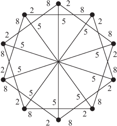
The complexity of the overall MCSD test can be clearly improved if we consider the possible isomorphism between graphs generated from distinct valid label sets. We say that two distinct labelings $\lambda$ and $\lambda^{\prime}$ are equivalent, denoted by $\lambda\equiv\lambda^{\prime}$, if they generate isomorphic graphs. For example, it can be easily seen that the labelings $\lambda$ and $\lambda^{\prime}$, drawing respectively on the label sets $\{1,2,5\}$ and $\{3,4,5\}$, generate isomorphic $5$-regular graphs on $10$ vertices (see Figure 5), so $\lambda\equiv\lambda^{\prime}$. Let us then consider a transformation of $\lambda$ into $\lambda^{\prime}$ that preserves the MCSD property. In what follows, $\lambda$ draws on the set $\{\gamma_{1},\ldots,\gamma_{\left\lceil k/2\right\rceil}\}$ for labels, $\lambda^{\prime}$ on $\{\gamma_{1}^{\prime},\ldots,\gamma_{\left\lceil k/2\right\rceil}^{\prime}\}$.

It is easy to see that any $\alpha>n/2$ would produce the same results as its symmetric modulo $n$. We can also see that any $\lambda$ comprising a $\gamma_{i}$ such that $\gamma_{i}\perp n$ can yield a $\lambda^{\prime}$ with $\gamma_{i}^{\prime}=1$. For such, it is sufficient to take $\alpha$ as the multiplicative inverse (modulo $n$) of $\gamma_{i}$.

It is also curious to note that the transformation in Theorem 10 ensures that $\gamma_{i}\perp n$ if and only if $\gamma_{i}^{\prime}\perp n$. To see this, consider for example the case of $\gamma_{i}^{\prime}=\alpha\mathrel{{\mathop{\cdot}}_{n}}\gamma_{i}$. By using Euclid’s Theorem [14] and the fact that $\alpha\perp n$ in succession, we have $\gcd(\alpha\mathrel{{\mathop{\cdot}}_{n}}\gamma_{i},n)=\gcd(\alpha\gamma_{i},n)=\gcd(\gamma_{i},n)$, thence $\gcd(\gamma_{i}^{\prime},n)=\gcd(\gamma_{i},n)$.

There is a clear equivalence between circulant graphs and regular graphs that admit an MCSD. We describe it formally in the following theorem.

One first example of how Theorem 11 sheds new light on the two concepts involved comes from considering the result on circulant graphs in [3], which implies in the connected case that $\gcd(s_{0},\ldots,s_{k},n)=1$, where $s_{i}$, for $0\leq i\leq k$, is an element of the set of generators. This is of course coherent with Lemma 7 and Corollary 9, and a straightforward implication of the general result of [3] is that a circulant graph is Hamiltonian if and only if it is connected [7]. Our approach introduces new ways of constructing Hamiltonian cycles in this case.

Another interesting insight is the following. An $n\times n$ matrix is said to be circulant if its $i$th line is the cyclic shift of the first line by $i$ positions, where $0\leq i\leq n-1$. Another characterization of circulant graphs is that a graph is circulant if its adjacency matrix is circulant. By the equivalence established in Theorem 11, it then becomes possible to approach the problem of recognizing regular graphs that admit an MCSD along a different route: since it is well-known that the isomorphism between two graphs $G$ and $H$ can be viewed as a permutation of lines and columns of the adjacency matrix of $G$ ($A(G)$) that generates that of $H$, we can test whether a regular graph $G$ admits an MCSD by finding a permutation of lines and columns of $A(G)$ such that the resulting matrix is circulant.

We note, in addition, that the transformation defined in Theorem 10 also has an analogue in the literature on circulant graphs. Let $G$ and $H$ be circulant graphs such that their sets of generators are $R$ and $S$, respectively. We say that $R$ and $S$ are $proportional$, denoted by $R\sim S$, if, for some $a\perp n$, $r=a\mathrel{{\mathop{\cdot}}_{n}}s$ bijectively for $r\in R$ and $s\in S$. Clearly, if $R\sim S$ then $G$ is isomorphic to $H$. The converse statement was conjectured in [1] and is known as Ádám’s conjecture. However, in [8] the conjecture was proven false.

The problem of recognizing circulant graphs, finally, is probably the one most affected by the equivalence of Theorem 11. Even though the algorithm we suggest to test whether a $k$-regular graph admits an MCSD is polynomial only for fixed $k$, when applied to the context of circulant graphs it is the only known result on arbitrary topologies (without any restrictions on the structure or the number of vertices) for that class.

References

- [1] A. Ádám. Research problem 2-10. Journal of Combinatorial Theory, 2:393, 1967.
- [2] J. C. Bermond, F. Cornellas, and D. F. Hsu. Distributed loop computer networks: a survey. Journal of Parallel and Distributed Computing, 24:2–10, 1995.
- [3] F. Boesch and R. Tindell. Circulants and their connectivities. Journal of Graph Theory, 8:487–499, 1984.
- [4] P. Boldi and S. Vigna. Minimal sense of direction and decision problems for Cayley graphs. Information Processing Letters, 64:299–303, 1997.
- [5] P. Boldi and S. Vigna. On the complexity of deciding sense of direction. SIAM Journal on Computing, 29(3):779–789, 2000.
- [6] J. A. Bondy and U. S. R. Murty. Graph Theory with Applications. North-Holland, New York, NY, 1976.
- [7] R. E. Burkard and W. Sandholzer. Efficiently solvable special cases of bottleneck travelling salesman problems. Discrete Applied Mathematics, 32:61–76, 1991.
- [8] B. Elspas and J. Turner. Graphs with circulant adjacency matrices. Journal of Combinatorial Theory, 9:297–307, 1970.
- [9] G. Fertin and A. Raspaud. Recognizing recursive circulant graphs. Electronic Notes in Discrete Mathematics, 5, 2000.
- [10] P. Flocchini. Minimal sense of direction in regular networks. Information Processing Letters, 61:331–398, 1997.
- [11] P. Flocchini, B. Mans, and N. Santoro. On the impact of sense of direction on message complexity. Information Processing Letters, 63(1):23–31, 1997.
- [12] P. Flocchini, B. Mans, and N. Santoro. Sense of direction: definitions, properties and classes. Networks, 32(3):165–180, 1998.
- [13] P. Flocchini, B. Mans, and N. Santoro. Sense of direction in distributed computing. Theoretical Computer Science, 291:29–53, 2003.
- [14] R. L. Graham, D. E. Knuth, and O. Patashnik. Concrete Mathematics: A Foundation for Computer Science. Addison-Wesley, Boston, MA, 2 edition, 1994.
- [15] E. M. Luks. Isomorphism of graphs of bounded valence can be tested in polynomial time. Journal of Computer and System Sciences, 25(1):42–65, 1982.
- [16] M. Muzychuk and G. Tinhofer. Recognizing circulant graphs of prime order in polynomial time. The Electronic Journal of Combinatorics, 3:108–111, 1996.
- [17] M. Muzychuk and G. Tinhofer. Recognizing circulant graphs in polynomial time: an application of association schemes. The Electronic Journal of Combinatorics, 8, 2001.
- [18] N. Santoro. Sense of direction, topological awareness and communication complexity. SIGACT News, 2(16):50–56, 1984.