Pseudo-Codewords of Cycle Codes via Zeta Functionsdummytext

Ralf Koetter Coordinated Science Lab.
University of Illinois
Urbana, IL 61801
koetter@uiuc.edu Wen-Ching W. Li Department of Mathematics
Pennsylvania State University
University Park, PA 16802-6401
wli@math.psu.edu Pascal O. Vontobel Coordinated Science Lab.
University of Illinois
Urbana, IL 61801
vontobel@ifp.uiuc.edu Judy L. Walker Department of Mathematics
University of Nebraska
Lincoln, NE 68588-0130
jwalker@math.unl.edu Note: dummytext Note: dummytext Note: dummytext Note: dummytext

Pseudo-Codewords of Cycle Codes via Zeta Functions⁰⁰ 0 dummytext

Ralf Koetter¹¹ 1 dummytext

Coordinated Science Lab.
University of Illinois
Urbana, IL 61801
koetter@uiuc.edu

Wen-Ching W. Li²² 2 dummytext

Department of Mathematics
Pennsylvania State University
University Park, PA 16802-6401
wli@math.psu.edu

Pascal O. Vontobel³³ 3 dummytext

Coordinated Science Lab.
University of Illinois
Urbana, IL 61801
vontobel@ifp.uiuc.edu

Judy L. Walker⁴⁴ 4 dummytext

Department of Mathematics
University of Nebraska
Lincoln, NE 68588-0130
jwalker@math.unl.edu

⁰⁰footnotetext: This is essentially the paper that was presented at the IT Workshop 2004, San Antonio, TX, USA. We replaced “Newton polytope” by “Newton polyhedron” throughout the text and corrected a slight unpreciseness in Th. V.4¹¹footnotetext: R. Koetter’s research was partially supported by NSF Grants CCR 99-84515 and CCR 01-05719.²²footnotetext: W.-C. W. Li’s research was partially supported by NSA Grant MDA904-03-1-0069.³³footnotetext: P. O. Vontobel is now with the ECE Dept., University of Wisconsin-Madison, USA, vontobel@ece.wisc.edu; his research was partially supported by NSF Grants CCR 99-84515 and CCR 01-05719.⁴⁴footnotetext: J. L. Walker’s research was partially supported by NSF Grant DMS 03-02024.

Abstract — Cycle codes are a special case of low-density parity-check (LDPC) codes and as such can be decoded using an iterative message-passing decoding algorithm on the associated Tanner graph. The existence of pseudo-codewords is known to cause the decoding algorithm to fail in certain instances. In this paper, we draw a connection between pseudo-codewords of cycle codes and the so-called edge zeta function of the associated normal graph and show how the Newton polyhedron of the zeta function equals the fundamental cone of the code, which plays a crucial role in characterizing the performance of iterative decoding algorithms.

I. Introduction

We are interested in characterizing the performance of a binary low-density parity-check (LDPC) code $C$ used for the transmission of information over a memoryless channel. Moreover, we focus on the case that iterative decoding is performed at the receiver end.

Let the code be described by a parity-check matrix $H$ . To a matrix $H$ we can associate a bipartite graph, the so-called Tanner graph $T\triangleq T(H)$ [1]. As was realized in [2], an essential role in the understanding of iterative decoding is played by the finite covers of the Tanner graph $T$ and the codes defined by them. In fact, while the main strength of iterative decoders, namely their low complexity, results from the fact that they operate locally on the Tanner graph, this very fact is also the source of the weakness of any iterative decoding algorithm. The systemic problem is that by just performing local operations the decoder cannot distinguish if it is decoding on the Tanner graph $T$ or any of the finite covers. Thus, codewords in a cover of $T$ will be interfering with the iterative decoding process. Consequently, in order to understand the behavior of iterative decoders we will have to characterize the “covering” codes and their codewords.

The goal of this paper is to give a concise geometric and simple description of these codes in finite covers of $T$ . In particular, the geometric characterization will relate to a cone in Euclidean space, the so-called fundamental cone [2].

We focus on a special class of LDPC codes, namely the class of cycle codes. These codes are informally defined as LDPC codes where all bit nodes have degree two.⁵⁵ 5 The reason for the name “cycle codes” will become clear in Sec. Pseudo-Codewords of Cycle Codes via Zeta Functions.

From a practical point of view cycle codes are somewhat marred by the fact that their minimum distance grows (at best) logarithmically in the block length (assuming fixed check-node degrees). Nevertheless, their properties make them more amenable to analysis than general LDPC codes. In any case, cycle codes can be seen as an interesting object of study from which results can (hopefully) be suitably generalized to the more interesting class of LDPC codes where part or all of the bit nodes have degree at least three.

The connections between iterative decoding and LDPC codes are probably best understood for cycle codes. First of all, the fundamental cone can be related concisely to the decoding behavior under iterative decoding, and secondly, as we aim to show in this paper, the fundamental cone may be identified as the Newton polyhedron of Hashimoto’s edge zeta function [11] associated to the normal graph (defined in Sec. Pseudo-Codewords of Cycle Codes via Zeta Functions) of the code. For an early reference about the performance of iterative decoding techniques in conjunction with cycle codes see [4, ch.6]. In the case of general LDPC codes, the relation of the fundamental cone to the exact characterization of the iterative decoding behavior is more intricate. Nevertheless, even here the fundamental cone gives an amazingly exact picture of the behavior.⁶⁶ 6 The behavior of the linear programming decoder [3] (for the most canonical relaxation) is exactly characterized by the fundamental cone in the cycle code case and in the non-cycle code case. While we here only establish the connection between the fundamental cone and the edge zeta function for cycle codes, we conjecture the existence of such a zeta function for the case of general LDPC codes.

This paper is structured as follows: Sec. Pseudo-Codewords of Cycle Codes via Zeta Functions introduces the basics about Tanner graphs and normal graphs of binary linear codes and Sec. Pseudo-Codewords of Cycle Codes via Zeta Functions discusses graph covers and the fundamental cone associated with a code. The notion of an edge zeta function of a graph will be introduced in Sec. Pseudo-Codewords of Cycle Codes via Zeta Functions and Sec. Pseudo-Codewords of Cycle Codes via Zeta Functions discusses the main result of this paper, namely the identification of the fundamental cone and the Newton polyhedron in the case of cycle codes. Throughout the whole paper we will use two running examples containing two different codes, namely Code A and Code B: the first is not a cycle code whereas the latter one is a cycle code.

II. Binary Linear Codes and Their Graphs

Definition II.1.

An undirected graph $X=X(V(X),E(X))$ consists of a vertex-set $V\triangleq V(X)$ and an edge-set $E\triangleq E(X)$ where the elements of $E$ are 2-subsets of $V$ . We assume a fixed ordering on $E$ so that $E=\{e_{1},\dots,e_{n}\}$ , where $n\triangleq n(X)\triangleq|E|$ . By a graph (without further qualifications) we will always mean an undirected graph. We will not allow self-loops or multiple edges. For $v\in V$ , we write ${\partial}(v)$ for the neighborhood of $v$ , i.e., the collection of vertices of $X$ which are adjacent to $v$ .

Definition II.2.

Let⁷⁷ 7 Note the following convention: a row index of $H$ will be denoted by $j$ and a column index of $H$ will be denoted by $i$ . $H=(h_{ji})$ be the parity-check matrix of a binary linear code $C$ . We let $J\triangleq J(H)$ be the set of row indices of $H$ and we let $I\triangleq I(H)$ be the set of column indices of $H$ , respectively. For each $i\in I$ , we let $J_{i}\triangleq J_{i}(H)\triangleq\big\{j\in J\ |\ h_{ji}{=}1\big\}$ . For each $j\in J$ , we let $I_{j}\triangleq I_{j}(H)\triangleq\big\{i\in I\ |\ h_{ji}{=}1\big\}$ . Furthermore, for any $I^{\prime}\subseteq I$ and any vector $\mathbf{x}$ of length $|I|$ , we let $\mathbf{x}_{I^{\prime}}$ be the vector that has only the entries of $\mathbf{x}$ whose indices are in $I^{\prime}$ . The Tanner graph [1] (or factor graph [5]) associated to $H$ will be called $T(H)$ : it consists of bit nodes $X_{1},\ldots,X_{|I|}$ , (parity-)check nodes $p_{1},\ldots,p_{|J|}$ , and edges between the two types of nodes. More precisely, bit node $i$ and check node $j$ are connected if and only if $h_{ji}=1$ . The degree of bit node $i$ is the number of adjacent check nodes in $T(H)$ and is therefore equal to $|J_{i}(H)|$ . The degree of check node $j$ is the number of adjacent bit nodes in $T(H)$ and is therefore equal to $|I_{j}(H)|$ . We say that a vector $\mathbf{x}\in\mathbb{F}_{2}^{|I|}$ is a configuration of the Tanner graph $T(H)$ and we call $\mathbf{x}\in\mathbb{F}_{2}^{|I|}$ a valid configuration if all the checks are fulfilled, i.e. $\sum_{i\in I}h_{ji}x_{i}=\sum_{i\in I_{j}}x_{i}=0\text{ (in $\mathbb{F}_{2}$)}$ for all $j\in J$ . Obviously, the set of all valid configurations forms the linear binary code $C$ .

Definition II.3.

A binary linear code $C$ defined by a parity-check matrix $H$ is called a cycle code if the associated Tanner graph $T(H)$ is $2$ -regular in the bit nodes, i.e. all bit nodes have degree $2$ . This is equivalent to the condition that for all $i\in I(H)$ we have $|J_{i}(H)|=2$ . Such codes were studied e.g. in [6].

Refer to caption — Figure 1: (Code A) Left: Tanner graph $T(H)$ of the simple binary linear code in Ex. II.4. Right: Tanner graph of an example of an $M$ -cover of $T(H)$ .

Example II.4 (Code A).

Let $C$ be a binary $[4,2]$ code with parity-check matrix

\displaystyle H

\displaystyle\triangleq\begin{pmatrix}1&1&1&0\\ 0&1&1&1\end{pmatrix}.

Obviously, $C=\big\{(0,0,0,0),(0,1,1,0),(1,0,1,1),(1,1,0,1)\big\}$ , $J=\{1,2\}$ , $J_{1}=\{1\}$ , $J_{2}=\{1,2\}$ , $J_{3}=\{1,2\}$ , $J_{4}=\{2\}$ , $I=\{1,2,3,4\}$ , $I_{1}=\{1,2,3\}$ , and $I_{2}=\{2,3,4\}$ . The Tanner graph $T(H)$ that is associated to $H$ is shown in Fig. 1 (left); it can easily be seen that this is not a cycle code.

Example II.5 (Code B).

Let $C$ be a binary $[7,2]$ code with parity-check matrix

\displaystyle H

\displaystyle\triangleq\begin{pmatrix}1&1&0&0&0&0&0\\ 0&1&1&1&0&0&0\\ 1&0&1&0&0&0&0\\ 0&0&0&1&1&0&1\\ 0&0&0&0&1&1&0\\ 0&0&0&0&0&1&1\end{pmatrix}.

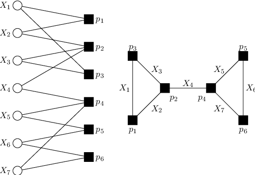
Obviously, $C=\big\{(0,0,0,0,0,0,0),(1,1,1,0,0,0,0),(0,0,0,0,$ $1,1,1),(1,1,1,0,1,1,1)\big\}$ .⁸⁸ 8 Note that the rank of $H$ is $5$ and not $6$ : therefore the dimension of $C$ is $2$ and not $1$ . The Tanner graph $T(H)$ of $C$ is shown in Fig. 2 (left). As can easily be seen, all bit nodes have degree $2$ and so the code $C$ is a cycle code. From the Tanner graph $T(H)$ we can derive another graph $N(H)$ in the following way: replace each (degree- $2$ ) bit node and its adjacent edges by a single edge and label the new edge according to the labeling of the bit node in the Tanner graph.⁹⁹ 9 We gave the label $N(H)$ because such a graph is also known as normal graph or Forney-style factor graph [7]. For code $C$ we obtain the graph $N(H)$ shown in Fig. 2 (right). From this graph the notion of “cycle code” becomes clear: every codeword (i.e. every valid configuration) corresponds to a simple cycle or a symmetric difference set of simple cycles in the normal graph. This will be made more precise in Sec. Pseudo-Codewords of Cycle Codes via Zeta Functions.

III. The Fundamental Cone

The following definition introduces the graph theoretic notion of a “graph cover”.

Definition III.1.

[8, 9] An unramified, finite cover, or, simply, a cover of a graph $X$ is a graph $Y$ along with a surjective map $\pi:Y\to X$ which is a graph homomorphism, i.e., which takes adjacent vertices of $Y$ to adjacent vertices of $X$ , such that for each vertex $x$ of $X$ and each $y\in\pi^{-1}(x)$ , the neighborhood ${\partial}(y)$ of $y$ is mapped bijectively to ${\partial}(x)$ . For a positive integer $M$ , an $M$ -cover of $X$ is an unramified finite cover $\pi:Y\to X$ such that for each vertex $x$ of $X$ , $\pi^{-1}(x)$ contains exactly $M$ vertices of $Y$ .

Example III.2 (Code A).

We continue with Code A defined in Ex. II.4. Let $T\triangleq T(H)$ be the Tanner graph corresponding to $H$ . An $M$ -fold cover $\widetilde{T}$ (as shown in Fig. 1 (right)) of $T$ is specified by defining the permutations $\pi_{1,1}$ , $\pi_{1,2}$ , $\pi_{1,3}$ (corresponding to the first row of $H$ ) and the permutations $\pi_{2,2}$ , $\pi_{2,3}$ , $\pi_{2,4}$ (corresponding to the second row of $H$ ).

The parity-check matrix $\widetilde{H}$ associated to one possible $3$ -fold cover Tanner graph $\widetilde{T}$ looks like

	$\displaystyle\widetilde{H}$	$\displaystyle\triangleq\left(\begin{array}[]{ccc\|ccc\|ccc\|ccc}0&1&0&1&0&0&0&1&0&0&0&0\\ 0&0&1&0&1&0&0&0&1&0&0&0\\ 1&0&0&0&0&1&1&0&0&0&0&0\\ \hline\cr 0&0&0&0&0&1&0&0&1&1&0&0\\ 0&0&0&1&0&0&1&0&0&0&1&0\\ 0&0&0&0&1&0&0&1&0&0&0&1\end{array}\right)$
		$\displaystyle=\begin{pmatrix}I_{2}&I_{0}&I_{2}&0\\ 0&I_{1}&I_{1}&I_{0}\end{pmatrix},$

where $I_{s}$ is a $3\times 3$ identity matrix, cyclically shifted to the left by $s$ positions. This parity-check matrix defines a code $\widetilde{C}$ : an example of a codeword of $\widetilde{C}$ is $\mathbf{\widetilde{c}}=(1,1,0,\ 0,1,1,\ 0,1,1,\ 0,0,0)$ .

Other examples of a graph cover are shown in Fig. 3: the left-hand side shows a double cover Tanner graph of the Tanner graph in Fig. 2 (left) and the right-hand side shows the corresponding double cover normal graph of the normal graph in Fig. 2 (right). The following remark formalizes Ex. III.2.

Remark III.3.

Let $C$ be a binary code with parity-check matrix $H$ and Tanner graph $T\triangleq T(H)$ . Let $J\triangleq J(H)$ and $I_{j}\triangleq I_{j}(H)$ . For a positive integer $M$ , let $\widetilde{T}$ be an arbitrary $M$ -fold cover of $T$ and let $\widetilde{C}$ be the binary code described by $\widetilde{T}$ . Knowing the graph $T$ , the graph $\widetilde{T}$ is completely specified by defining for all $j\in J$ and all $i\in I_{j}$ the permutations $\pi_{j,i}$ that map $[M]\triangleq\{1,\ldots,M\}$ onto itself. The meaning of $\pi_{j,i}(m)$ , $m\in[M]$ is the following: the $m^{\text{th}}$ copy of the check node $j$ is connected to the $\pi_{j,i}(m)^{\text{th}}$ copy of the $i^{\text{th}}$ bit. It follows that $\mathbf{\widetilde{c}}\in\widetilde{C}$ if and only if

\displaystyle\sum_{i\in I_{j}}\widetilde{c}_{i,\pi_{j,i}(m)}

\displaystyle=0\hskip 9.24994pt\text{(in $\mathbb{F}_{2}$)}

for all $j\in J$ and all $m\in[M]$ . The parity-check matrix $\widetilde{H}$ that expresses this fact can be defined as follows. Let the entries of $\widetilde{H}$ be indexed by $(j,m)\in J\times[M]$ and $(i,m^{\prime})\in I\times[M]$ . Then

\displaystyle h_{(j,m),(i,m^{\prime})}

\displaystyle\triangleq\begin{cases}1&\text{if $i\in I_{j}$ and $m^{\prime}=\pi_{j,i}(m)$}\\ 0&\text{otherwise}.\end{cases}

Definition III.4.

[2] Let $C$ be a binary linear (base) code with parity-check matrix $H$ and let $T\triangleq T(H)$ be the corresponding Tanner graph. For any positive integer $M$ , let $\widetilde{T}$ be an $M$ -fold cover of $T$ and let $\widetilde{C}$ be the binary code described by $\widetilde{T}$ . We will denote a codeword of $\widetilde{C}$ by $\mathbf{\widetilde{c}}$ , where the $(i,m)$ ’s component of $\mathbf{\widetilde{c}}$ , i.e. $\widetilde{c}_{i,m}$ , denotes the value of the $m^{\text{th}}$ copy of the $i^{\text{th}}$ bit.

The pseudo-codeword associated to $\mathbf{\widetilde{c}}$ is the rational vector $\boldsymbol{\omega}(\mathbf{\widetilde{c}})\triangleq\big(\omega_{1}(\mathbf{\widetilde{c}}),\omega_{2}(\mathbf{\widetilde{c}}),\ldots,\omega_{n}(\mathbf{\widetilde{c}})\big)$ with

\displaystyle\omega_{i}(\mathbf{\widetilde{c}})

\displaystyle\triangleq\frac{1}{M}\sum_{m\in[M]}\widetilde{c}_{i,m},

where the sum is taken in $\mathbb{R}$ (not in $\mathbb{F}_{2}$ ). We call the vector $M\cdot\boldsymbol{\omega}(\mathbf{\widetilde{c}})$ the unscaled pseudo-codeword associated with $\mathbf{\widetilde{c}}$ . In fact, any multiple (by a positive scalar) of $\boldsymbol{\omega}(\mathbf{\widetilde{c}})$ will be called a pseudo-codeword associated with $\mathbf{\widetilde{c}}$ .

Note that any codeword is also a pseudo-codeword.

Remark III.5.

Notice that a pseudo-codeword, as defined in Def. III.4, has length $|I(H)|$ , the same as the length of any codeword, whereas a codeword like $\mathbf{\widetilde{c}}\in\widetilde{C}$ has length $M\cdot|I(H)|$ , where $M$ is the degree of the corresponding cover Tanner graph.

Example III.6 (Code A).

We continue with Code A defined in Ex. II.4. We saw that $\mathbf{\widetilde{c}}=(1,1,0,\ 0,1,1,\ 0,1,1,\ 0,0,0)$ was a codeword of the code $\widetilde{C}$ . Applying Def. III.4 we see that the corresponding pseudo-codeword is $\boldsymbol{\omega}(\mathbf{\widetilde{c}})=(\frac{2}{3},\frac{2}{3},\frac{2}{3},0)$ and that the corresponding unscaled pseudo-codeword is $3\cdot\boldsymbol{\omega}(\mathbf{\widetilde{c}})=(2,2,2,0)$ . Note that $\boldsymbol{\omega}(\mathbf{\widetilde{c}})$ cannot be written as a convex combination of the codewords in $C$ .

The influence of a pseudo-codeword on the decoding behavior under iterative decoding can be measured by its pseudo-weight which is a function of the pseudo-codeword and the channel used (see [2] and references therein). An important property of the pseudo-weight is its scaling invariance, i.e. scaling a pseudo-codeword by a positive scalar leaves its pseudo-weight unchanged.

The fundamental cone that is given in the following definition will be, along with the zeta functions of a graph, a main object of interest in this paper.

Definition III.7.

[2, 3] Let $C$ be an arbitrary binary linear code and let $H$ be its parity-check matrix. We define the fundamental cone ${K}(H)$ of $H$ to be the set of vectors $\boldsymbol{\omega}\in\mathbb{R}^{n}$ that satisfy

	$\displaystyle\forall i\in I:$		$\displaystyle\hskip 9.24994pt\omega_{i}$	$\displaystyle\geq 0,$
	$\displaystyle\forall j\in J,\ \forall i\in I_{j}:$		$\displaystyle\hskip 9.24994pt\sum_{i^{\prime}\in I_{j}\setminus\{i\}}\omega_{i^{\prime}}$	$\displaystyle\geq\omega_{i},$

where $J\triangleq J(H)$ , $I\triangleq I(H)$ , $I_{j}\triangleq I_{j}(H)$ .

Example III.8 (Code A).

We continue with Code A defined in Ex. II.4. The fundamental cone ${K}(H)$ is the set

	$\displaystyle{K}(H)=\{(\omega_{1},\omega_{2},$	$\displaystyle\omega_{3},\omega_{4})\in\mathbb{R}^{4}\big\|\,\omega_{1}\geq 0,\omega_{2}\geq 0,\omega_{3}\geq 0,\omega_{4}\geq 0,$
		$\displaystyle-\omega_{1}+\omega_{2}+\omega_{3}\geq 0,\ \ \ -\omega_{2}+\omega_{3}+\omega_{4}\geq 0,$
		$\displaystyle+\omega_{1}-\omega_{2}+\omega_{3}\geq 0,\ \ \ +\omega_{2}-\omega_{3}+\omega_{4}\geq 0,$
		$\displaystyle+\omega_{1}+\omega_{2}-\omega_{3}\geq 0,\ \ \ +\omega_{2}+\omega_{3}-\omega_{4}\geq 0\}.$

The next two lemmas establish that there is a very tight connection between the fundamental cone of a code and codewords that live in finite covers. More specifically, in one direction we prove that the pseudo-codeword associated to any codeword in a cover of a Tanner graph must lie within the fundamental polytope. In the other direction we prove that to a given vector in the fundamental polytope we can find a cover with a codeword in it whose (suitably scaled) pseudo-codeword is arbitrarily close to the given vector.

Lemma III.9.

[2] Let $C$ be a binary linear code with parity-check matrix $H$ and Tanner graph $T=T(H)$ . For a positive integer $M$ , let $\widetilde{T}$ be an arbitrary $M$ -fold cover of $T$ and let $\widetilde{C}$ be the binary code described by $\widetilde{T}$ . If $\mathbf{\widetilde{c}}\in\widetilde{C}$ then $\boldsymbol{\omega}(\mathbf{\widetilde{c}})\in{K}(H)$ .

Lemma III.10.

[2] Let $C$ be a binary linear code with parity-check matrix $H$ and Tanner graph $T=T(H)$ . Let the vector $\boldsymbol{\omega}^{\prime}\in\mathbb{R}^{n}$ satisfy $\boldsymbol{\omega}^{\prime}\in{K}(H)$ . Then for any $\varepsilon>0$ , there is a positive integer $M$ such that there is a codeword $\mathbf{\widetilde{c}}$ in a code $\widetilde{C}$ defined by an $M$ -fold cover $\widetilde{T}$ of $T$ such that $||\alpha\boldsymbol{\omega}(\mathbf{\widetilde{c}})-\boldsymbol{\omega}^{\prime}||_{2}<\varepsilon$ for some $\alpha>0$ .

Putting Lemmas III.9 and III.10 together, we have:

Theorem III.11.

Let $C$ be a binary linear code with parity-check matrix $H$ and fundamental cone ${K}(H)$ . Then the lines through the pseudo-codewords for $C$ are dense in ${K}(H)$ . ∎

Moreover, we have

Theorem III.12.

The point $\boldsymbol{\omega}=(\omega_{1},\dots,\omega_{|I|})\in K(H)\cap{\mathbb{Z}}^{n}$ is an unscaled pseudo-codeword if and only if $\sum_{i\in I}h_{ji}\omega_{i}=0\text{ (in $\mathbb{F}_{2}$)}$ for each $j\in J$ .

Proof.

This follows from Lemma III.10 and Corollary V.5. ∎

IV. Zeta Functions of Graphs

Before we can talk about zeta functions of graphs we need to say exactly what we mean by a cycle in a graph.

Definition IV.1.

Let $X$ be an undirected graph as in Def. II.1. A sequence $(e_{i_{1}},\dots,e_{i_{k}})$ of edges of $X$ is a cycle on $X$ if the edges $e_{i_{j}}$ can be directed so that $e_{i_{s}}$ terminates where $e_{i_{s+1}}$ begins for $1\leq s\leq k-1$ and $e_{i_{k}}$ terminates where $e_{i_{1}}$ begins. The characteristic vector of the cycle $(e_{i_{1}},\dots,e_{i_{k}})$ on $X$ is the binary vector of length $n$ whose $t^{\text{th}}$ coordinate is 1 if and only if $e_{t}$ appears as some $e_{i_{j}}$ . If the cycle does not cross itself, i.e., if each vertex of $X$ is involved in at most two of the edges $e_{i_{1}}$ , …, $e_{i_{k}}$ , then we say the cycle is simple.

This definition relates as follows to the cycle codes introduced in Sec. Pseudo-Codewords of Cycle Codes via Zeta Functions:

Lemma IV.2.

Let $N\triangleq N(H)$ be the normal graph of a binary cycle code $C$ with parity-check matrix $H$ . The characteristic vector of any simple cycle in $N$ is a valid configuration of $N$ , i.e. it is a codeword of $C$ . Moreover, the symmetric difference of the characteristic vector of simple cycles in $N$ is also a valid configuration of $N$ , i.e. it is a codeword of $C$ . On the other hand, to any codeword in $C$ corresponds the symmetric difference of simple cycles in $N$ .

Proof.

This follows from Euler’s Theorem [10, Th. 1.2.26]. ∎

The code $C$ in Lemma IV.2 can also be seen as spanned by the characteristic vectors of the simple cycles of $N$ . The length of $C$ equals $n(N)$ , the number of edges in $N$ . Further, the minimum Hamming distance $d_{\mathrm{min}}$ of $C$ is the length of the shortest cycle in $N$ , i.e., the girth of $N$ . Also, the dimension of $C$ is the number of independent cycles in $N$ , i.e., the rank of the fundamental group of the underlying topological space of $N$ , i.e., $|E(N)|-|V(N)|+1=1-\chi(N)$ , where $\chi(N)$ is the Euler characteristic of $N$ .

Let us turn back to graph-theoretic notions: the next important step is to introduce a special class of cycles called “primitive, backtrackless and tailless cycles”.

Definition IV.3.

Let $\Gamma=(e_{i_{1}},\dots,e_{i_{k}})$ be a cycle in a graph $X$ . We say $\Gamma$ is backtrackless if for no $s$ do we have $e_{i_{s}}=e_{i_{s+1}}$ . We say $\Gamma$ is tailless if $e_{i_{1}}\neq e_{i_{k}}$ . We say $\Gamma$ is primitive if there is no cycle $\Theta$ on $X$ such that $\Gamma=\Theta^{r}$ with $r\geq 2$ , i.e., such that $\Gamma$ is obtained by following $\Theta$ a total of $r$ times. We say that the cycle $\Psi=(e_{j_{1}},\dots,e_{j_{k}})$ is equivalent to $\Gamma$ if there is some integer $t$ such that $e_{j_{s}}=e_{j_{(s+t)\ \operatorname{mod}\ k}}$ for all $s$ .

It is easy to check that any simple cycle is a primitive, backtrackless and tailless cycle and that the notion of equivalence given in Def. IV.3 defines an equivalence relation on primitive, backtrackless, tailless cycles.

Example IV.4 (Code B).

Let us return to Code B defined in Ex. II.5 and its normal graph shown in Fig. 2 (right); the edge with variable label $X_{i}$ will be called $e_{i}$ . We see that the edge-sequences $(e_{1},e_{2},e_{3})$ and $(e_{5},e_{6},e_{7})$ are simple cycles: they correspond to the codewords $(1,1,1,0,0,0,0)$ and $(0,0,0,0,1,1,1)$ , respectively, in $C$ .

In contrast to these two cycles, the cycles

	$\displaystyle\Gamma_{1}$	$\displaystyle=(e_{1},e_{2},e_{4},e_{5},e_{6},e_{7},e_{4},e_{3})$
	$\displaystyle\Gamma_{2}$	$\displaystyle=(e_{3},e_{4},e_{7},e_{6},e_{5},e_{4},e_{2},e_{1})$
	$\displaystyle\Gamma_{3}$	$\displaystyle=(e_{1},e_{2},e_{4},e_{5},e_{6},e_{7},e_{5},e_{6},e_{7},e_{4},e_{3})$

are not simple cycles; but they are inequivalent, backtrackless, tailless, primitive cycles. Indeed, we can obtain infinitely many inequivalent, backtrackless, tailless, primitive cycles on $N(H)$ by, for example, following the path $(e_{1},e_{2},e_{4})$ , then arbitrarily many copies of the loop $(e_{5},e_{6},e_{7})$ , and then $(e_{4},e_{3})$ .

The edge zeta function of a graph is a way to enumerate all inequivalent, primitive, backtrackless cycles and combinations thereof.

Definition IV.5.

[11, 9] Let $\Gamma$ be a path in a graph $X$ with edge-set $E$ ; write $\Gamma=(e_{i_{1}},\dots,e_{i_{k}})$ to indicate that $\Gamma$ begins with the edge $e_{i_{1}}$ and ends with the edge $e_{i_{k}}$ . The monomial of $\Gamma$ is given by $g(\Gamma)\triangleq u_{i_{1}}\cdots u_{i_{k}}$ , where the $u_{i}$ ’s are indeterminates. The edge zeta function of $X$ is defined to be the power series $\zeta_{X}(u_{1},\dots,u_{n})\in{\mathbb{Z}}[[u_{1},\dots,u_{n}]]$ given by

\displaystyle\zeta_{X}(u_{1},\dots,u_{n})

\displaystyle=\prod_{[\Gamma]\in A(X)}\big(1-g(\Gamma)\big)^{-1},

where $A(X)$ is the collection of equivalence classes of backtrackless, tailless, primitive cycles in $X$ .

As Ex. IV.4 shows, the product in the definition of the edge zeta function is, in general, infinite. However, it is true that the edge zeta function is a rational function. To see this, we first need a few more definitions.

Definition IV.6.

[9] Let $X=(V(X),E(X))$ be an undirected graph with edge set $E(X)=\{e_{1},\ldots,e_{n}\}$ . A directed graph $\vec{X}=(\vec{V}(\vec{X}),\vec{E}(\vec{X}))$ derived from $X$ is a graph with vertex set $\vec{V}(\vec{X})\triangleq V(X)$ and edge set $\vec{E}(\vec{X})\triangleq\{f_{1},\dots,f_{2n}\}$ , where the (directed) edges $f_{i}$ and $f_{n+i}$ both correspond to the same edge $e_{i}\in E(X)$ but have opposite directions.

Definition IV.7.

[9] Let $\vec{X}=(\vec{V}(\vec{X}),\vec{E}(\vec{X}))$ be a directed graph as defined in Def. IV.6. The directed edge matrix of $\vec{X}$ is the matrix $M(\vec{X})=(m_{ij})$ where

\displaystyle m_{ij}

\displaystyle=\begin{cases}1,&\text{if $f_{i}$ feeds into $f_{j}$ to form a backtrackless path}\\ 0,&\text{otherwise.}\end{cases}

Example IV.8 (Code B).

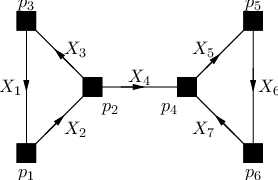
Let us continue with Code B defined in Ex. II.5. The normal graph $N=N(H)$ of the code is shown in Fig. 2 (right); the edge with variable label $X_{i}$ will be called $e_{i}$ . The directed edges $f_{1}$ to $f_{14}$ of a directed version $\vec{N}$ of $N$ are chosen such that the edges $f_{1}$ to $f_{7}$ are as shown in Fig. 4. Implicitly this figure also defines the edges $f_{8}$ to $f_{14}$ ; e.g., $f_{11}$ is the same as $f_{4}$ but directed from right to left. The directed edge matrix $M\triangleq M(\vec{N})$ of $\vec{N}$ is then the matrix

\displaystyle M

\displaystyle=\left[\begin{array}[]{ccccccc|ccccccc}0&1&0&0&0&0&0&0&0&0&0&0&0&0\\ 0&0&1&1&0&0&0&0&0&0&0&0&0&0\\ 1&0&0&0&0&0&0&0&0&0&0&0&0&0\\ 0&0&0&0&1&0&0&0&0&0&0&0&0&1\\ 0&0&0&0&0&1&0&0&0&0&0&0&0&0\\ 0&0&0&0&0&0&1&0&0&0&0&0&0&0\\ 0&0&0&0&1&0&0&0&0&0&1&0&0&0\\ \hline\cr 0&0&0&0&0&0&0&0&0&1&0&0&0&0\\ 0&0&0&0&0&0&0&1&0&0&0&0&0&0\\ 0&0&0&1&0&0&0&0&1&0&0&0&0&0\\ 0&0&1&0&0&0&0&0&1&0&0&0&0&0\\ 0&0&0&0&0&0&0&0&0&0&1&0&0&1\\ 0&0&0&0&0&0&0&0&0&0&0&1&0&0\\ 0&0&0&0&0&0&0&0&0&0&0&0&1&0\end{array}\right].

With these definitions, Stark and Terras [9] prove:

Theorem IV.9.

[9] The edge zeta function $\zeta_{X}(u_{1},\dots,u_{n})$ is a rational function. More precisely, for any directed graph $\vec{X}$ of $X$ , we have

\displaystyle\zeta_{X}(u_{1},\dots,u_{n})^{-1}

\displaystyle=\det(I-UM(\vec{X}))=\det(I-M(\vec{X})U)

where $I$ is the identity matrix of size $2n$ and $U=\mathop{\text{diag}}(u_{1},\dots,u_{n},u_{1},\dots,u_{n})$ is a diagonal matrix of indeterminants.

Example IV.10 (Code B).

Let us continue with Code B defined in Ex. II.5 and its normal graph $N\triangleq N(H)$ . By the above theorem and using $\vec{N}$ from Ex. IV.8, the edge zeta function $\zeta_{N}$ of our graph $N$ satisfies

	$\displaystyle\zeta_{N}$	$\displaystyle(u_{1},\dots,u_{7})^{-1}=\det(I_{14}-UM)=\det(I_{14}-MU)$
		$\displaystyle=1-2u_{1}u_{2}u_{3}+u_{1}^{2}u_{2}^{2}u_{3}^{2}-2u_{5}u_{6}u_{7}+4u_{1}u_{2}u_{3}u_{5}u_{6}u_{7}$
		$\displaystyle\phantom{spa}-2u_{1}^{2}u_{2}^{2}u_{3}^{2}u_{5}u_{6}u_{7}-4u_{1}u_{2}u_{3}u_{4}^{2}u_{5}u_{6}u_{7}$
		$\displaystyle\phantom{spa}+4u_{1}^{2}u_{2}^{2}u_{3}^{2}u_{4}^{2}u_{5}u_{6}u_{7}+u_{5}^{2}u_{6}^{2}u_{7}^{2}-2u_{1}u_{2}u_{3}u_{5}^{2}u_{6}^{2}u_{7}^{2}$
		$\displaystyle\phantom{spa}+u_{1}^{2}u_{2}^{2}u_{3}^{2}u_{5}^{2}u_{6}^{2}u_{7}^{2}+4u_{1}u_{2}u_{3}u_{4}^{2}u_{5}^{2}u_{6}^{2}u_{7}^{2}$
		$\displaystyle\phantom{spa}-4u_{1}^{2}u_{2}^{2}u_{3}^{2}u_{4}^{2}u_{5}^{2}u_{6}^{2}u_{7}^{2}.$

Expanding out the Taylor series, we get the first several terms of $\zeta_{N}$ :

	$\displaystyle\zeta_{N}$	$\displaystyle(u_{1},\dots,u_{7})=1+2u_{1}u_{2}u_{3}+3u_{1}^{2}u_{2}^{2}u_{3}^{2}+2u_{5}u_{6}u_{7}$
		$\displaystyle\phantom{spa}+4u_{1}u_{2}u_{3}u_{5}u_{6}u_{7}+6u_{1}^{2}u_{2}^{2}u_{3}^{2}u_{5}u_{6}u_{7}$
		$\displaystyle\phantom{spa}+4u_{1}u_{2}u_{3}u_{4}^{2}u_{5}u_{6}u_{7}+12u_{1}^{2}u_{2}^{2}u_{3}^{2}u_{4}^{2}u_{5}u_{6}u_{7}$
		$\displaystyle\phantom{spa}+3u_{5}^{2}u_{6}^{2}u_{7}^{2}+6u_{1}u_{2}u_{3}u_{5}^{2}u_{6}^{2}u_{7}^{2}+9u_{1}^{2}u_{2}^{2}u_{3}^{2}u_{5}^{2}u_{6}^{2}u_{7}^{2}$
		$\displaystyle\phantom{spa}+12u_{1}u_{2}u_{3}u_{4}^{2}u_{5}^{2}u_{6}^{2}u_{7}^{2}+36u_{1}^{2}u_{2}^{2}u_{3}^{2}u_{4}^{2}u_{5}^{2}u_{6}^{2}u_{7}^{2}+\cdots.$

V. Relating the Fundamental Cone and the Zeta Function of a Cycle Code

The results of this chapter are based on the simple observations made in the following example.

Example V.1 (Code B).

Let us continue with Code B defined in Ex. II.5 and its Tanner graph $T\triangleq T(H)$ as shown in Fig. 2 (left). We saw that any codeword corresponds one-to-one to a valid configuration in $T$ .

Consider now a double cover $\widetilde{T}$ of $T$ as shown in Fig. 3 (left): the set of all valid configurations of $\widetilde{T}$ defines a code $\widetilde{C}$ . Because of the properties of graph covers, the code $\widetilde{C}$ is again a cycle code and in the same manner as in Ex. II.5 we deduce its normal graph $\widetilde{N}$ . It is not hard to see that $\widetilde{N}$ shown in Fig. 3 (right) is a double cover of the normal graph $N\triangleq N(H)$ shown in Fig. 2 (right).

Just as the codewords of $C$ correspond bijectively to the vectors in the span of the characteristic vectors of the simple cycles in $N$ , the codewords of $\widetilde{C}$ correspond bijectively to the vectors in the span of the characteristic vectors of the simple cycles in $\widetilde{N}$ .

An example of simple cycle in $\widetilde{N}$ is the edge-sequence¹⁰¹⁰ 10 The edge with variable label $X^{\prime}_{i}$ ( $X^{\prime\prime}_{i}$ ) will be called $e^{\prime}_{i}$ ( $e^{\prime\prime}_{i}$ ).

\displaystyle\widetilde{\Gamma}

\displaystyle=(e^{\prime}_{1},e^{\prime}_{2},e^{\prime\prime}_{4},e^{\prime\prime}_{5},e^{\prime\prime}_{6},e^{\prime}_{7},e^{\prime}_{4},e^{\prime}_{3}).

After mapping it down to $N$ it reads

\displaystyle\pi(\widetilde{\Gamma})

\displaystyle=(e_{1},e_{2},e_{4},e_{5},e_{6},e_{7},e_{4},e_{3}),

which is a backtrackless and tailless cycle in $N$ which is not simple. Note that in general the image of a simple cycle is always backtrackless and tailless, but not necessarily simple or primitive. The cycle $\widetilde{\Gamma}$ corresponds to a codeword $\mathbf{\widetilde{c}}$ and the mapped cycle $\pi(\widetilde{\Gamma})$ corresponds to the pseudo-codeword

\displaystyle\boldsymbol{\omega}(\mathbf{\widetilde{c}})

\displaystyle=\frac{1}{2}\cdot(1,1,1,2,1,1,1)=\left(\frac{1}{2},\frac{1}{2},\frac{1}{2},1,\frac{1}{2},\frac{1}{2},\frac{1}{2}\right).

With this example we can draw the following important conclusion about cycle codes (which will be formalized in Th. V.4): listing the pseudo-codewords stemming from all the possible finite covers is equivalent to listing all backtrackless and tailless cycles of the normal graph and combinations thereof. But listing these cycles (in a certain way) is exactly what the zeta function of the normal graph essentially does!

Definition V.2.

The exponent vector of the monomial $u_{1}^{p_{1}}\dots u_{n}^{p_{n}}$ is the vector $(p_{1},\dots,p_{n})\in{\mathbb{N}}_{0}^{n}$ of the exponents of the monomial.

Example V.3 (Code B).

Continuing with Code B that was defined in Ex. II.5 and the zeta function $\zeta_{N}$ of its normal graph $N\triangleq N(H)$ (cf. Ex. IV.10), we see that the exponent vectors of the first several monomials appearing in $\zeta_{N}$ are (0,0,0,0,0,0,0), (1,1,1,0,0,0,0), (2,2,2,0,0,0,0), (0,0,0,0,1,1,1), (1,1,1,0,1,1,1), (2,2,2,0,1,1,1), (1,1,1,2,1,1,1), (2,2,2,2,1,1,1), (0,0,0,0,2,2,2), (1,1,1,0,2,2,2), (2,2,2,0,2,2,2), (1,1,1,2,2,2,2), (2,2,2,2,2,2,2), …. Note that most of these lie within the span of multiples of codewords in $C$ ; for example,

\displaystyle(1,1,1,0,2,2,2)

\displaystyle=(1,1,1,0,0,0,0)+2(0,0,0,0,1,1,1).

The exceptions thus far are (1,1,1,2,1,1,1), (2,2,2,2,1,1,1), (1,1,1,2,2,2,2) and (2,2,2,2,2,2,2). The first of these exceptions is exactly the pseudo-codeword for $C$ given in Ex. V.1, and the rest lie within the span of this pseudo-codeword along with multiples of codewords.

These observations are made precise in the next theorem.

Theorem V.4.

Let $C$ be a cycle code defined by a parity-check matrix $H$ having normal graph $N\triangleq N(H)$ , let $n=n(N)$ be the number of edges of $N$ , and let $\zeta_{N}(u_{1},\dots,u_{n})$ be the edge zeta function of $N$ . Then the monomial $u_{1}^{p_{1}}\dots u_{n}^{p_{n}}$ has nonzero coefficient in $\zeta_{N}$ if and only if the corresponding exponent vector $(p_{1},\dots,p_{n})$ is an unscaled pseudo-codeword for $C$ .

Sketch of proof.

By Def. IV.5, the monomial $u_{1}^{p_{1}}\dots u_{n}^{p_{n}}$ appears with nonzero coefficient in $\zeta_{N}$ if and only if there are backtrackless, tailless, primitive cycles $\Gamma_{1},\dots,\Gamma_{m}$ on $X$ such that

\displaystyle u_{1}^{p_{1}}\dots u_{n}^{p_{n}}

\displaystyle=g(\Gamma_{1})^{q_{1}}\cdots g(\Gamma_{m})^{q_{m}}

for some nonnegative integers $q_{1},\dots,q_{m}$ . It is thus enough to prove that $\Gamma$ is a backtrackless, tailless cycle on $N$ if and only if $\Gamma=\pi(\widetilde{\Gamma})$ for some simple cycle $\widetilde{\Gamma}$ on some (finite, unramified) cover $\widetilde{N}$ of $N$ , where $\pi:\ \widetilde{N}\to N$ is the canonical surjection.

So, first suppose that $\pi:\ \widetilde{N}\to N$ is a cover of $N$ and that $\widetilde{\Gamma}$ is a simple cycle on $\widetilde{N}$ . We must show that $\pi(\widetilde{\Gamma})$ is a backtrackless, tailless cycle on $N$ . Suppose otherwise, namely, that $(x,y,x)$ is part of the vertex sequence of $\pi(\widetilde{\Gamma}^{\prime})$ for some $\widetilde{\Gamma}^{\prime}$ equivalent to $\widetilde{\Gamma}$ . Then it comes from $(\widetilde{u},\widetilde{v},\widetilde{w})$ in $\widetilde{\Gamma}^{\prime}$ . In particular, this means that $v$ is adjacent to two distinct vertices $\widetilde{u}$ and $\widetilde{w}$ in $\widetilde{N}$ , both of which project to $x$ . This cannot happen in a finite unramified cover. Thus $\pi(\widetilde{\Gamma})$ is backtrackless and tailless.

For the converse, we must show that given a backtrackless, tailless cycle $\Gamma$ on $N$ , there is a cover $\pi:\ \widetilde{N}\to N$ and a simple cycle $\widetilde{\Gamma}$ on $\widetilde{N}$ lifting $\Gamma$ . This is done by induction on the length of $\Gamma$ , with cycles of length $3$ , which are necessarily simple, providing the base case. For a nonsimple cycle $\Gamma$ of length greater than $3$ , the idea is to break off the first simple cycle $\Gamma_{1}$ appearing within $\Gamma$ . Then $\Gamma$ is equivalent to a composition of $\Gamma_{1}$ with some other cycle $\Gamma_{2}$ which has length less than that of $\Gamma$ . If $\Gamma_{2}$ is backtrackless, then it has a lift to a simple cycle by induction hypothesis and one must explicitly show how to “glue together” this lift with the cycle $\Gamma_{1}$ to form a simple lifting of $\Gamma$ . The case where $\Gamma_{2}$ has backtracking presents a bit more difficulty, but is handled similarly. ∎

The following corollary is contained in the proof of Th. V.4.

Corollary V.5.

Consider the same setup as in Th. V.4. The vector $p=(p_{1},...,p_{n})\in{\mathbb{N}}^{n}$ is an unscaled pseudo-codeword for $C$ if and only if there is a backtrackless tailless cycle in $X$ which uses the $i^{\text{t}h}$ edge exactly $p_{i}$ times for $1\leq i\leq n$ . Moreover, the unscaled pseudo-codewords of $C$ are in one-to-one correspondence with the monomials appearing with nonzero coefficient in the edge zeta function $\zeta_{N}$ of $N$ . Finally, the Newton polyhedron of $\zeta_{N}$ (i.e. the polyhedron spanned by the exponents of the terms in the Taylor series of $\zeta_{N}$ ) equals the fundamental cone ${K}(H)$ of the code $C$ .

References

[1] R. M. Tanner, “A recursive approach to low-complexity codes,” IEEE Trans. on Inform. Theory, vol. IT–27, pp. 533–547, Sept. 1981.
[2] R. Koetter and P. O. Vontobel, “Graph covers and iterative decoding of finite-length codes,” in Proc. 3rd Intern. Conf. on Turbo Codes and Related Topics, (Brest, France), pp. 75–82, Sept. 1–5 2003. Available online under http://www.ifp.uiuc.edu/~vontobel.
[3] J. Feldman, D. R. Karger, and M. J. Wainwright, “LP decoding,” in Proc. 41st Allerton Conf. on Communications, Control, and Computing, (Allerton House, Monticello, Illinois, USA), October 1–3 2003. Available online under http://www.columbia.edu/~jf2189/pubs.html.
[4] N. Wiberg, “Codes and Decoding on General Graphs”, Linköping Studies in Science and Technology, Ph.D thesis No. 440, Linköping, Sweden. http://www.it.isy.liu.se/ publikationer/LIU-TEK-THESIS-440.pdf.
[5] F. R. Kschischang, B. J. Frey, and H.-A. Loeliger, “Factor graphs and the sum-product algorithm,” IEEE Trans. on Inform. Theory, vol. IT–47, no. 2, pp. 498–519, 2001.
[6] S. L. Hakimi and J. Bredeson, “Graph-theoretic error correcting codes,” IEEE Trans. on Inform. Theory, vol. IT–14, no. 4, pp. 584–591, 1968.
[7] G. D. Forney, Jr., “Codes on graphs: normal realizations,” IEEE Trans. on Inform. Theory, vol. 47, no. 2, pp. 520–548, 2001.
[8] W. S. Massey, Algebraic Topology: an Introduction. New York: Springer-Verlag, 1977. Reprint of the 1967 edition, Graduate Texts in Mathematics, Vol. 56.
[9] H. M. Stark and A. A. Terras, “Zeta functions of finite graphs and coverings,” Adv. Math., vol. 121, no. 1, pp. 124–165, 1996.
[10] D. B. West, Introduction to graph theory. Upper Saddle River, NJ: Prentice Hall Inc., 1996.
[11] K. Hashimoto, “Zeta functions of finite graphs and representations of $p$ -adic groups,” in Automorphic forms and geometry of arithmetic varieties, vol. 15 of Adv. Stud. Pure Math., pp. 211–280, Boston, MA: Academic Press, 1989.