Stochastic Iterative Decoders
Abstract
This paper presents a stochastic algorithm for iterative error control decoding. We show that the stochastic decoding algorithm is an approximation of the sum-product algorithm. When the code’s factor graph is a tree, as with trellises, the algorithm approaches maximum a-posteriori decoding. We also demonstrate a stochastic approximations to the alternative update rule known as successive relaxation. Stochastic decoders have very simple digital implementations which have almost no RAM requirements. We present example stochastic decoders for a trellis-based Hamming code, and for a Block Turbo code constructed from Hamming codes.
I Introduction
Iterative decoding describes a class of powerful graph-based algorithms for error control decoding, including Turbo and LDPC decoders. Implementations tend to be complex, and much research effort has been invested to produce less complex physical solutions [1, 2, 3, 4].
We describe implementation strategies in terms of parallel and serial architectures. The parallel approach requires large numbers of small processors which operate concurrently. This approach consumes a large amount of silicon area.
In serial architectures, processors are reused multiple times within an iteration, thus requiring use of a RAM for storing messages. This approach requires less silicon area, but reduces the decoder’s maximum throughput. The serial approach is also expensive to apply in reconfigurable implementations, because RAM tends to be limited in current FPGA platforms.
In this paper, we present a stochastic approximation to the sum-product algorithm. This approximation allows for low-complexity parallel decoder implementations. The resulting circuits have no RAM requirements, and are simple enough to be implemented in low-cost FPGAs.
In stochastic implementations, each processor is implemented by a simple logic gate. The stochastic algorithm can therefore be implemented on a code’s factor graph, using only a few gates per node.
Similar algorithms have been presented elsewhere [5]. The stochastic decoding algorithm is related to Pearl’s method of “stochastic simulation,” which provides accurate belief propagation in cyclic Bayesian networks [6]. Pearl’s method does not work for cyclic networks with deterministic constraints, and therefore cannot be used for error-control decoding.
In this paper, we present a new form of the stochastic algorithm which is more general than the original, strictly binary algorithm [5]. Unlike Pearl’s method, our goal is not to produce cycle-independent results, but to produce a low-complexity approximation of the sum-product decoding algorithm.
This paper is organized as follows. In Sec. II we present a review of notation and terminology. Sec. II-B summarizes the widely-used sum-product iterative update rule. Sec. II-C presents the less common successive relaxation update rule, a derivative of sum-product which sometimes yields better performance and/or faster convergence [7].
In Sec. III we describe the new stochastic decoding algorithm. Stochastic implementation on acyclic code graphs is discussed in Sec. III-B, which also presents results for a stochastic trellis decoder.
Cyclic constraint graphs require use of a modified node, called the supernode, which is discussed in Sec. III-C. This Section also presents results for a length-256 stochastic Block Turbo decoder.
Throughout the paper, significant results are presented as theorems. The proofs of these theorems are intended to be illustrative, but not fully rigorous.
II Message-Passing Decoding Algorithms
The conventional sum-product algorithm consists of probability propagation through nodes in a code’s factor graph [8]. For our purposes, we consider a more limited class of factor graphs called constraint graphs.
A constraint graph represents the relationships among a code’s variables and constraints. Constraint functions define which combinations of variables are permissible and which are not.
II-A Constraint graphs.
A constraint graph is a type of factor graph which shows the constraints among a code’s information and parity bits. The constraint graph consists of nodes and edges. Variables are usually represented by circles, and constraints (functions) are represented by squares.
It is customary to show information and parity bits explicitly as circles in the constraint graph. These variables represent observable information, and have a single edge connection.
A code is constructed from a family of constraint functions, represented in the graph by squares. For most codes of interest, all constraints may be expressed using functions of no more than three variables.
We now proceed to a more precise explanation of these concepts. Let , and be variables with alphabets , and , respectively. We denote particular values of , and using lower-case letters , and . Without loss of generality, we assume that , and are subsets of the natural numbers (including 0).
Let be defined by the Cartesian product . Let be a Boolean function, , and define the set . The function induces mappings , and , defined by
The mappings and are defined similarly.
If , and are all functions, then is said to be a constraint function. For some combination , if then the constraint is said to be satisfied. It is sometimes convenient to refer to the set as the satisfaction of the constraint function .
A constraint function has a one-to-one correspondence with its satisfaction. The satisfaction can be written as a table with three columns, which we call the satisfaction table.
The satisfaction table corresponds to a trellis graph, which consists of two columns of states and a set of branches connecting between them. On the left of the trellis, the states correspond to the alphabet . The states on the right correspond to . The branches in the middle are labeled with symbols from . For each row in the satisfaction table, there is a branch in the trellis which connects with , and which is labeled . This relationship is illustrated by Fig. 1.
When we present a constraint graph, we include an unlabeled trellis graph for each constraint node. This trellis graph indicates the structure and complexity of the corresponding constraint function.

|
| ||||||||||||||||||||||||||||
| A. | B. |
II-B The sum-product update rule.
The sum-product algorithm replaces each variable in the constraint graph with a random variable. The task is then to compute the (conditional) probability mass of one variable, given the available independent (conditional) probability masses of all other variables.
Each edge in the graph is then associated with two probability masses, because each edge is connected to two nodes. Each function node produces, for every edge, a unique estimate of the (conditional) probability mass, based on the information which appears at the other edges. Probability masses are generally represented by vectors, and may sometimes be represented by summary messages, such as log-likelihood ratios or soft bits.
Let , and be the conditional probability mass vectors for variables , and , respectively, and let denote the element of . Define as the set . For most applications, the sum-product algorithm is described by the equation
| (1) |
The proportionality symbol in (1) is used to indicate that the resulting mass vector must be normalized so that the sum is equal to one. Let be the union . The normalized sum-product equation is then
| (2) | |||||
The node update rule (2) is used to update the message transmitted on each edge from each function node.
Throughout this paper, we will assume the use of a “flooding” schedule for message passing. In this schedule, all nodes receive messages at the start of each iteration. They compute updated messages on each edge, and then complete the iteration by transmitting the updated messages.
II-C The relaxation update rule.
In the conventional sum-product algorithm, a node’s outgoing messages are replaced by a new probability mass determined according to (2). One alternative to replacement is the method of successive relaxation [7], which we refer to simply as relaxation.
Let be the mass estimated according to (2). Also let refer to the mass produced by relaxation at time , and let be the mass produced by relaxation at time . Then the relaxation update rule is described by
| (3) |
where is referred to as the relaxation parameter, .
The relaxation method produces smoother updating than the replacement method. It has been shown that relaxation (3) is equivalent to Euler’s method for simulating differential equations. It has also been shown that the relaxation method results in superior performance for some codes.
III The Stochastic Algorithm
The stochastic decoding algorithm is a message-passing algorithm. Like the sum-product algorithm, it is based on the code’s constraint graph. In the stochastic algorithm, messages are not probability mass vectors. Stochastic messages are integers which change randomly according to some probability mass.
Stochastic messages can be regarded as sequences of integers. The probability mass is communicated over time by the sequence. One mass corresponds to many possible sequences.
At each discrete time instant , a function node, , receives messages , and , and transmits messages , and . The integer messages vary randomly over time, according to the probability masses , and , respectively. The message therefore equals integer with probability . All probabilities lie in the open interval .
III-A The stochastic update rule.
To implement the stochastic message-passing algorithm, we use the following deterministic message update rule at each function node. We consider the propagation of message from to . Suppose that, at time , and . Then
| (4) |
We claim that the stochastic update rule (4) produces a message with mass which is equal to the mass computed by the sum-product update rule (2). To support this claim, we rely upon the following assumptions:
- 1.
There is no correlation between any pair of sequences received by a constraint node.
- 2.
The probability mass associated with any message sequence is stationary.
When a node is considered in isolation from the graph, the above conditions apply.
Theorem 1
A node receives stochastic messages and , and transmits a message according to the update rule (4). The received messages have stationary probability masses and . Then the mass of the transmitted message, , is equal to the result computed by the sum-product update rule.
Proof:
The probability of transmitting a particular integer is
We assume that the mass of each variable is stationary. Then . Therefore
which is the same as (2). ∎The stochastic update rule (4) results in very simple node implementations. The implementation of a node consists of a logic gate which is precisely as complex as the node’s trellis description.
III-B Message-passing implementation on acyclic graphs.
For a constraint graph with no cycles, a complete stochastic decoder is constructed by applying the update rule (4) to every constraint node. Probability masses, representing the channel information, are stored at the variable nodes. The variable nodes generate the first messages randomly, according to the channel information.
The random integer messages flow deterministically through the decoder, through a cascade of constraint nodes, until they arrive back at the variable nodes. The messages are tabulated in histograms as they arrive at the variable nodes. After time-steps, the variable nodes make decisions by selecting the symbol with the largest count.
When implemented in this way, the assumptions of Sec. III-A are never violated. The probability mass of each message in the decoder is therefore equivalent to that of the sum-product algorithm. By increasing , the result of stochastic decoding can be made arbitrarily close to that of sum-product decoding.
Example 1
An acyclic constraint graph for a (16, 11) Hamming code is shown in Fig. 2. A stochastic decoder is constructed by replacing each constraint node with logic gates, according to the update rule (4). We allow time-steps for decoding. The performance of the resulting code for antipodal transmission on a Gaussian channel is shown in Fig. 3.


III-C Graphs with cycles and Supernodes.
If the constraint graph contains one or more cycles, then the assumptions of Sec. III-A are violated. In particular, the independence among received messages , and no longer holds for some or all constraint nodes.
When the messages at a node are correlated, it is possible for a group of nodes to settle into a fixed state. This state is maintained solely by the messages within the cycle. No pattern of independent messages is sufficient to restore the cycle to proper functioning. We refer to this phenomenon as latching.
A simple latching example is the all-zero state in an LDPC graph. If all internal messages between parity and equality nodes are zero, then they will be held permanently at zero, regardless of any activity from the variable nodes.
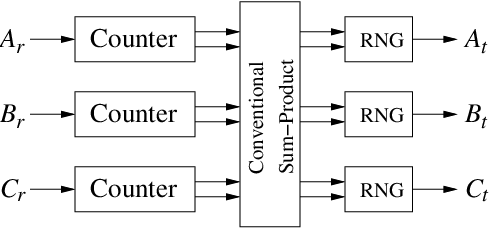
To avoid latching, cycles may be interrupted with a special stochastic node, called a supernode. A supernode receives stochastic messages and tabulates them in histograms. It then generates new messages based on the estimated probability masses, resulting in a new uncorrelated sequence.
A supernode can be implemented with counters and a linear feedback shift-register (LFSR) to generate random numbers. The simplest supernode implementation is illustrated in Fig. 4.

We also claim that the supernode must be packetized, which is defined as follows. Suppose a supernode is generating a random sequence according to an estimated mass . We say that the supernode’s behavior is packetized if the estimated mass is only updated every time-steps. During these time-steps, the supernode tabulates the received message(s). After the time-step, is updated with the newly tabulated information.
Data received during the time-steps is called a packet, and the -step time interval is called an iteration. There are two obvious procedures by which may be updated:
- 1.
The tabulation is cleared after each iteration, and the mass estimate is replaced by a new estimate representing only the data from the most recent packet.
- 2.
The tabulation is not cleared after each packet of time-steps. The tabulation is accumulated over many iterations until decoding is complete.
For sufficiently large , these supernode update rules approach the behavior of sum-product and relaxation updates, respectively.
Theorem 2
Suppose each cycle in a stochastic constraint graph contains a supernode, and the mass estimated by the supernode is updated by replacement every time-steps. Then the result of stochastic decoding approaches that of sum-product decoding as is increased.
Proof:
Let be the total number of observations of an event , and let be the total number of observations for which . By definition for a stationary mass , . The mass of is is therefore estimated with arbitrarily small error as is increased.
The messages produced by the supernode have a fixed mass, and are therefore stationary. They are also not correlated with any other messages in the graph. Theorem 1 therefore applies, and the stochastic decoder approaches the behavior of a sum-product iteration for large . ∎
Theorem 3
Suppose each cycle in a stochastic constraint graph contains a supernode, and the mass estimated by the supernode is updated by accumulation every time-steps. Then the result of stochastic decoding approaches that of relaxation, where the relaxation parameter varies as , where is the number of iterations.
Proof:
Let be a supernode’s newly updated estimate of the mass of an event just after iterations, and let be the supernode’s estimate after iterations. The supernode has made total observations. Let be number of observations in the packet for which . Let be the number of observations in the first packets for which . Then the new estimate is
| (5) | |||||
As , approaches the sum-product estimate of for the iteration. Upon substitution, we find that (5) approaches the relaxation update rule with . The difference between relaxation and (5) can be made arbitrarily small by increasing . ∎
Example 2
The (16,11) Hamming code graph of Ex. 1 can be used to construct a (256,121) Block Turbo Code. The decoder for this code consists of 32 Hamming decoders, arranged in 16 rows and 16 columns. Each row shares precisely one bit with each column. Where two decoders share a bit, they are joined by an equality constraint.

The equality constraints create cycles in the constructed graph. To resolve this, we implement each equality node as a supernode. Within the equality supernode, received messages are converted to probability mass estimates. Using these mass estimates, the outgoing masses are computed using the conventional sum-product update rule (2). New stochastic sequences are generated to conform to the outgoing mass estimate.
We choose a flooding schedule with an accumulation update rule, and a packet length of . Eight iterations are allowed, for a total decoding time of 2000 time-steps. The stochastic decoder’s performance is as shown in Fig. 7. Also shown is the simulated performance of a commercial Block Turbo decoder from Comtech/Advanced Hardware Architectures [9]. The AHA decoder uses 26 iterations for decoding, and six bits of precision for the channel samples.

IV Discussion and Conclusions
While this paper validates that stochastic iterative decoding can be applied to interesting codes (e.g., Block Turbo codes), it also raises an interesting set of ancillary questions. There are numerous alternative stochastic update rules and message schedules, and many possible simplifications to the algorithm. Questions also remain concerning the relationships among the packet size, the number of iterations and the performance of a stochastic decoder for a given graph.
These issues hint at a broad set of interesting research questions, with significant potential to improve the complexity of iterative decoders.
References
- [1] M. Bekooij, J. Dielissen, F. Harmsze, S. Sawitzki, J. Huisken, A. van der Werf, and J. van Meerbergen, “power-efficient application-specific VLIW processor for Turbo decoding,” in Proc. 2001 IEEE International Solid State Circuits Conference (ISSCC’01), Feb. 2001, pp. 180–181.
- [2] J. Hagenauer and M. Winklhofer, “The analog decoder,” Proc. International Symposium on Information Theory, Aug. 1998.
- [3] Jagadeesh Kaza and Chaitali Chakrabarti, “Design and implementation of low-energy Turbo decoders,” IEEE Transactions on Very Large Scale Integration (VLSI) Systems, vol. 12, no. 9, pp. 968–977, Sept. 2004.
- [4] H. A. Loeliger, F. Lustenberger, M. Helfenstein, and F. Tarkoy, “Probability propagation and decoding in analog VLSI,” IEEE Transactions on Information Theory, vol. 47, no. 2, pp. 837–843, Feb. 2001.
- [5] Vincent C. Gaudet and Anthony C. Rapley, “Iterative decoding using stochastic computation,” Electronics Letters, vol. 39, no. 3, pp. 299–301, feb 2003.
- [6] Judea Pearl, Probabilistic Reasoning in Intelligent Systems : Networks of Plausible Inference, Morgan Kaufmann, 1988.
- [7] Saied Hemati and Amir H. Banihashemi, “On the dynamics of continuous-time analog iterative decoding,” in Proc. 2004 Int’l Symposium on Information Theory (ISIT 04), Chicago, June 2004, p. 262.
- [8] F. R. Kschischang, B. J. Frey, and H. A. Loeliger, “Factor graphs and the sum-product algorithm,” IEEE Transactions on Information Theory, vol. 47, no. 2, pp. 498–519, Feb. 2001.
- [9] Comtech AHA, “http://www.aha.com,” 2004.