跳到论文正文
W Papers独立论文阅读器 arXiv:cs/0411093 论文正文 计算阅读时间 · 0%
引用这篇论文根据当前论文元数据生成,正式投稿前建议核对。


License: Assumed arXiv.org perpetual non-exclusive license
arXiv:cs/0411093v1 [cs.DS] 25 Nov 2004

Forbidden Subgraphs in Connected Graphs Thanks: First version of this paper appeared in the 4-th Latin American Theoretical INformatics Conference – Punta del Este – Uruguay, April 2000 and some parts of this paper appeared in the 13-th International Conference on Formal Power Series and Algebraic Combinatorics – Arizona – USA, May 2001 (cf. RT00a; RT01a). This research was done while the first author was at LaRIA, Amiens – France.

Vlady Ravelomanana Address: LIPN UMR 7030, Université de Paris-Nord
99, Avenue J. B. Clément. F 93430 Villetaneuse France
   Loÿs Thimonier Address: LaRIA EA 2083, Université de Picardie
5, Rue du Moulin-Neuf. 80000 Amiens France
February 2002
Abstract

Given a set ξ={H1,H2,⋯}\xi=\{H_{1},H_{2},\cdots\} of connected non acyclic graphs, a ξ\xi-free graph is one which does not contain any member of ξ\xi as copy. Define the excess of a graph as the difference between its number of edges and its number of vertices. Let W^k,ξ{\widehat{W}}_{k,\xi} be theexponential generating function (EGF for brief) of connected ξ\xi-free graphs of excess equal to kk (k≥1k\geq 1). For each fixed ξ\xi, a fundamental differential recurrence satisfied by the EGFs W^k,ξ{\widehat{W}}_{k,\xi} is derived. We give methods on how to solve this nonlinear recurrence for the first few values of kk by means of graph surgery. We also show that for any finite collection ξ\xi of non-acyclic graphs, the EGFs W^k,ξ{\widehat{W}}_{k,\xi} are always rational functions of the generating function, TT, of Cayley’s rooted (non-planar) labelled trees. From this, we prove that almost all connected graphs with nn nodes and n+kn+k edges are ξ\xi-free, whenever k=o⁡(n1/3)k=o(n^{1/3}) and |ξ|<∞|\xi|<\infty by means of Wright’s inequalities and saddle point method. Limiting distributions are derived for sparse connected ξ\xi-free components that are present when a random graph on nn nodes has approximately n2\frac{n}{2} edges. In particular, the probability distribution that it consists of trees, unicyclic components, ⋯\cdots, (q+1)(q+1)-cyclic components all ξ\xi-free is derived. Similar results are also obtained for multigraphs, which are graphs where self-loops and multiple-edges are allowed.

Keywords: 
Combinatorial problems; enumerative combinatorics; analytic combinatorics; labelled graphs; multivariate generating functions; asymptotic enumeration; random graphs; triangle-free graphs.

1 Introduction

We consider here labelled graphs, i.e., graphs with labelled vertices, undirected edges and without self-loops or multiple edges as well as labelled multigraphs which are labelled graphs with self-loops and/or multiple edges. A (n,q)(n,q) graph (resp. multigraph) is one having nn vertices and qq edges.

On one hand, classical papers ER59; ER60; FKP89; JKLP93 provide algorithms and analysis of algorithms that deal with random graphs or multigraphs generation, estimating relevant characteristics of their evolution. Starting with an initially empty graph of nn vertices, we enrich it by successively adding edges. As random graph evolves, it displays a phase transition similar to the typical phenomena observed with percolation process. On the other hand, various authors such as Wright Wr77; Wr80 or Bender, Canfield and McKay BCM90; BCM92 studied exact enumeration or asymptotic properties of labelled connected graphs.

A lot of research is devoted to graphs not containing a prefixed set of subgraphs as copies and various approaches exist for these problems. Most of them, following Erdös and Rényi’s seminal papers ER59; ER60, are probabilistic; moment methods, tail inequalities, or probabilistic inequalities are then essential as well explained in Bollobas. These approaches take advantage over enumerative ones by allowing treatments under the edges independence assumption Bollobas. The situation changes radically if we consider connected components, and results relative to connectedness are few. Related works include Wr77; Wr78; Wr80; BCM90; BCM92; BCM97; FKP89; JKLP93

Let HH be a fixed connected graph; by a copy of HH, we mean any subgraph, not necessarily induced, isomorphic to HH. Let ℱ\mathcal{F} be a family of graphs none of which contains a copy of HH. In this case, we say that the family ℱ\mathcal{F} is HH-free. Otherwise, a graph containing a copy of HH is called a supergraph of HH. The highly non-trivial task of enumerating triangle-free or quadrilateral-free components goes back to the book of Harary and Palmer HP73.

Mostly forbidden configurations are triangle, quadrilateral, …, CpC_{p}, KpK_{p}, Kp,qK_{p,q} or any combination of them (see (Bollobas, Chapter IV), (JLR00, Chapter III)). CpC_{p} shall always denote the cycle on pp vertices, KpK_{p} the complete graph with pp vertices and Kp,qK_{p,q} the complete bipartite graph with pp vertices on the first side and qq vertices on the second side. For example, we can work with the family of graphs which do not contain a copy of triangle (C3C_{3}) or of K3,3K_{3,3}, i.e., {C3,K3,3}\{C_{3},K_{3,3}\}-free graphs. Following the authors of FKP89, we refer as bicyclic graphs all connected graphs with nn vertices and (n+1)(n+1) edges and in general (q+1)(q+1)-cyclic graphs are connected (n,n+q)(n,n+q) graphs. If we define the excess of a graph as the difference between its number of edges and its number of vertices, (q+1)(q+1)-cyclic graphs are referred also as qq-excess connected graphs. In general, we refer as multicyclic a connected graph which is not acyclic. The same nomenclature holds for multigraphs. More generally, denote by ξ={H1,H2,H3,…}\xi=\{H_{1},H_{2},H_{3},...\} a set of connected multicyclic graphs (resp. multigraphs); a ξ{\xi}-free graph is then one which does not contain any copy of HiH_{i} for all Hi∈ξH_{i}\in\xi as subgraph. Throughout this paper, unless explicitly mentioned, ξ\xi denotes a finite set of forbidden configurations.

Our aim in this paper is

  • 1.

    to study randomly generated graphs with nn vertex and approximately n2\frac{n}{2} edges focusing our attention on the appearance or not of the forbidden configurations,

  • 2.

    to compute the asymptotic number of ξ\xi-free connected graphs when ξ\xi is finite.

The results obtained here show that some characteristics of random generation as well as asymptotic enumeration of labelled graphs or multigraphs, can be read within the forms of the exponential generating functions (EGF for short) of the sparse components. In fact, denote by W^k\widehat{W}_{k} (k≥−1k\geq-1) the EGFs of (k+1)(k+1)-cyclic (connected) graphs. In a series of important papers, Wr77; Wr78; Wr80, E. M. Wright proved that W^k​(z)\widehat{W}_{k}(z) (k≥1)(k\geq 1), where zz is the variable marking the number of vertices in the graph, can be expressed as finite sums of power of 1/(1−T⁡(z))1/(1-T(z)) where T⁡(z)=∑n≥1nn−1​znn!T(z)=\sum_{n\geq 1}n^{n-1}\frac{z^{n}}{n!} is the EGF for rooted labelled trees Cay89; Moo67. Starting with a functional equation satisfied by our (k+1)(k+1)-cyclic ξ\xi-free graphs; we will show that their EGF, denoted W^k,ξ\widehat{W}_{k,\xi}, have the same global forms as those of (k+1)(k+1)-cyclic graphs, i.e., W^k\widehat{W}_{k}. These forms will allow us to study random graphs without forbidden configurations and also to enumerate asymptotically connected components of these objects under some restrictions. Similar results related to multigraphs will be treated and carried along this paper, in parallel. Since our results concern graphs and multigraphs, we will be frequently assuming throughout this paper that the term component is the general term for connected graph as well as for connected multigraph.

1.1 Asymptotic number of ξ\xi-free (n,n+o⁡(n1/3))(n,n+o(n^{1/3})) components

In the first part of this paper, we will compute the asymptotic number of triangle-free connected (n,n+k)(n,n+k)-graphs, whenever k=o⁡(n1/3)k=o(n^{1/3}). To do this, we will rely heavily on the results in Wr80 to prove that the power series W^k,C3\widehat{W}_{k,C_{3}} satisfy the same inequalities as for W^k\widehat{W}_{k} which we shall call here “Wright’s inequalities”. Next, we will investigate the asymptotic behavior of the coefficient of znz^{n} in 1(1−T⁡(z))k⁡(n)\frac{1}{(1-T(z))^{k(n)}} (where TT is the EGF for Cayley’s rooted labelled trees) by means of saddle point method. The combination of these computations will permit us to show almost all connected (n,n+o⁡(n1/3))(n,n+o(n^{1/3})) graphs, i.e., connected graphs with nn vertices and n+o⁡(n1/3)n+o(n^{1/3}) edges are triangle-free. These asymptotic results are related to the interesting problems posed by Harary and Palmer in their reference book (see (HP73, Sect. 10.4, 10.5 and 10.6)). The purpose of this part is also to introduce methods by which the asymptotic number of connected ξ\xi-free (n,n+k)(n,n+k) graphs can be computed systematically, whenever k=o⁡(n1/3)k=o(n^{1/3}).

1.2 Forbidden subgraphs in random (n,n2)(n,\frac{n}{2}) components

The two models of graph evolution, explicitly introduced in FKP89, are considered in the second part of this note, in order to generate randomly graphs and multigraphs. We will study the structure of evolving graphs and multigraphs when edges are added one at time and at random, mainly looking at the presence or absence of certain configurations. In (JKLP93, Theorem 5), the authors proved that the probability that a random graph or multigraph with nn vertices and n2+O⁡(n1/3)\frac{n}{2}+O(n^{1/3}) edges has r1r_{1} bicyclic components, r2r_{2} tricyclic components, …, rqr_{q} (q+1)(q+1)-cyclic components and no components of higher-cyclic order is

(43)r23b1r1r1!b2r2r2!⋯bqrqrq!r!(2​r)!+O(n−13)\left(\frac{4}{3}\right)^{r}\sqrt{\frac{2}{3}}\frac{b_{1}^{r_{1}}}{r_{1}!}\frac{b_{2}^{r_{2}}}{r_{2}!}\cdots\frac{b_{q}^{r_{q}}}{r_{q}!}\frac{r!}{(2r)!}+O(n^{-\frac{1}{3}}) (1)

where r=r1+2​r2+⋯+q​rqr=r_{1}+2r_{2}+\cdots+qr_{q} and the bib_{i} are Wright’s constants also found by Louchard and Takács (b1=524,b2=516b_{1}=\frac{5}{24},\,b_{2}=\frac{5}{16},   …), and are involved in an important series of papers Lo84a; Lo84b; Vo87; Ta91a; Ta91b; JKLP93; Sp97; FPV98.

Given a finite collection ξ={H1,H2,H3,…,Hq}\xi=\{H_{1},H_{2},H_{3},...,H_{q}\} of multicyclic connected components, with slight modifications of the results in JKLP93, we show that for a random graph or multigraph with nn vertices and m⁡(n)=n2​(1+μ​n−13)m(n)=\frac{n}{2}(1+\mu n^{-\frac{1}{3}}) edges, |μ|≤n1/12|\mu|\leq n^{1/12} (in this paper, we will often choose μ=O⁡(n−13)\mu=O(n^{-\frac{1}{3}}) so m⁡(n)=n2+O⁡(n13)m(n)=\frac{n}{2}+O(n^{\frac{1}{3}})), the probability of finding only acyclic and unicyclic components without copy of HiH_{i}, ∀Hi∈ξ\forall H_{i}\in\xi, is asymptotically the same value as for “general” random graphs times exp(−∑k∈Θ12​p){\exp{\left(-\sum_{k\in\Theta}\frac{1}{2p}\right)}} where Θ\Theta is the subset (possibly empty) of the lengths of all polygons in ξ\xi: Θ={p,Hi∈ξ\Theta=\{p,H_{i}\in\xi and HiH_{i} is a pp-gon}\}. For example, if ξ={C3,C4}\xi=\{C_{3},C_{4}\}, Θ={3,4}\Theta=\{3,4\} and the probability that a random graph or a multigraph with nn vertices and n2+O⁡(n1/3)\frac{n}{2}+O(n^{1/3}) edges has only trees and unicyclic components without triangles or quadrilaterals as induced subgraphs is

23e−16−18∼0.6099⋯.\sqrt{\frac{2}{3}}e^{-\frac{1}{6}-\frac{1}{8}}\sim 0.6099\cdots\,. (2)

Recall that an elementary contraction of a graph GG is obtained by identifying two adjacent points xx and yy, that is, by the removal of xx and yy and the addition of a new point zz adjacent to those points to which xx or yy were adjacent. Then a graph G1G_{1} is contractible to a graph G2G_{2} if G2G_{2} can be obtained from G1G_{1} by a sequence of elementary contractions. We show that a sufficient condition to change the coefficient bib_{i}, for any i>0i>0, of (1) in this probability is to force ξ\xi to contains the entire family of graphs contractible to certain graphs H1,H2,⋯H_{1},H_{2},\cdots (in this case ξ\xi is infinite). We then give the corresponding probability.

The ideas of sections 4, 5 and 6 may be summarized by the figure 1.

Refer to caption
Figure 1: Summarizing sections 4, 5, 6 and the methods therein.

1.3 An outline of the paper

The rest of this paper is organized as follows. In section 2, we recall some useful definitions and notations of the stuff we will encounter along this document. In section 3, we will work with the example of bicyclic graphs. The enumeration of these graphs was discovered, as far as we know, independently by Bagaev Bag73 and by Wright Wr77. The purpose of this example is two-fold. First, it brings a simple new combinatorial point of view to the relationship between the generating functions of some integer partitions, on one hand, and graphs, on the other hand. Next, this example gives us ideas, regarding the simplest complex components, i.e., simplest non-acyclic components, of what will happen if we force our graphs to contain some specific configurations (especially the form of the generating functions). In section 4, we start giving the functional equation satisfied by our ξ\xi-free connected graphs involving also the first components containing copies of forbidden configurations. This equation is difficult to solve but leads to the general forms of the EGFs of all (k+1)(k+1)-cyclic ξ\xi-free components. In fact, general combinatorial techniques are presented and used to enumerate the first low-order cyclic triangle-free components. Section 5 presents methods to estimate asymptotically the number of connected components built with nn vertices and n+kn+k edges as n→∞n\rightarrow\infty and k→∞k\rightarrow\infty but k=o⁡(n1/3)k=o(n^{1/3}). The obtained results show that almost all (n,n+o⁡(n1/3))(n,n+o(n^{1/3})) connected components are triangle-free and the methods used show that this fact can be generalized to any finite set ξ\xi of forbidden subgraphs. We then turn on the computation of the probability of random graphs/multigraphs without forbidden configurations in section 6. Along this paper, triangle-free graphs will be treated as significant example but many results stand for any finite set ξ\xi of forbidden multicyclic graphs or multigraphs.

2 Notations

Definitions and tools are given in this section. Because they are mostly well known, they are quickly sketched. Powerful tools in all combinatorial approaches, generating functions will be used for our concern. If F⁡(z)F(z) is a power series, we write [zn]​F​(z)\left[z^{n}\right]F(z) for the coefficient of znz^{n} in F⁡(z)F(z). We say that F⁡(z)F(z) is the exponential generating function (EGF for brief) for a collection ℱ\mathcal{F} of labelled objects if n!​[zn]​F​(z)n!\left[z^{n}\right]F(z) is the number of ways to attach objects in ℱ\mathcal{F} that have nn elements (see for instance FZvC94 or Wi90).

The generating functions for labelled unrooted and labelled rooted trees are nice examples of EGFs. The mathematical theory of labelled trees, as first discussed by Cayley in 1889 Cay89 was concerned in their enumeration aspect. This study initiated the enumeration of labelled graphs. In fact, a labelled tree is a connected graph with nn vertices labelled from 11 to nn and n−1n-1 edges. It is well known that the number of such structures upon nn points is nn−2n^{n-2}. Let TT be the EGF for labelled rooted trees. A tree consists of a root to which is attached a set of rooted subtrees, thus

T⁡(z)=z⁡(∑n≥0T​(z)nn!)=∑n≥1nn−1​znn!.T(z)=z\left(\sum_{n\geq 0}\frac{T(z)^{n}}{n!}\right)=\sum_{n\geq 1}n^{n-1}\frac{z^{n}}{n!}\,. (3)

In (3), the exponent of the variable zz reflects the number of nodes. One can use bivariate exponential generating function to count labelled rooted trees. Throughout this paper, the variable zz is the variable recording the number of nodes and ww is the variable for the number of edges. For e.g., a tree with nn vertices is a connected graph with n−1n-1 edges and we have

T⁡(w,z)=z​exp⁡(w​T​(w,z))=∑n>0(w​n)n−1​znn!.T(w,z)=z\,\exp{\left(w\,T(w,z)\right)}=\sum_{n>0}(wn)^{n-1}\frac{z^{n}}{n!}\,. (4)

This bivariate EGF satisfies

T⁡(w,z)=T⁡(w​z)w.T(w,z)=\frac{T(wz)}{w}\,. (5)

We will denote by WkW_{k}, resp. W^k\widehat{W}_{k}, the EGF for labelled multicyclic connected multigraphs, resp. graphs, with kk edges more than vertices. For k≥1k\geq 1, these EGFs have been computed in Wr77 and in JKLP93. A connected graph is of excess kk which is always greater than or equal to −1-1. Let W^−1\widehat{W}_{-1} be the EGF of unrooted labelled trees. One can obtain at generating function level the relation

W^−1​(z)=∫0zT⁡(x)​d​xx,\widehat{W}_{-1}(z)=\int_{0}^{z}T(x)\frac{dx}{x}\,, (6)

which reflects the fact that any node of an unrooted tree can be taken as the root. The integration of (6) leads to the classical relation

W^−1​(z)=T⁡(z)−T​(z)22.\widehat{W}_{-1}(z)=T(z)-\frac{T(z)^{2}}{2}\,. (7)

It is convenient to work with bivariate EGFs and the bivariate EGFs that enumerate the family 𝒲^k\widehat{\mathcal{W}}_{k} of labelled kk-excess graphs, for all k≥−1k\geq-1, can be expressed using the corresponding univariate EGFs as follows

W^k​(w,z)=wk​W^k​(w​z).\widehat{W}_{k}(w,z)=w^{k}\widehat{W}_{k}(wz)\,. (8)

The factor wkw^{k} in the right side of (8) reflects the excess of the component, that is its number of edges minus its number of vertices. The same remark holds between the univariate and bivariate EGFs, WkW_{k}, of kk-excess multigraphs.

Without ambiguity, one can also associate a given configuration of labelled graph or multigraph with its EGF. For instance, a triangle can be labelled in only one way and we have the following informal relation

C3→C3​(w,z)=13!​w3​z3.C_{3}\rightarrow C_{3}(w,z)=\frac{1}{3!}w^{3}z^{3}\,. (9)

For any given multicyclic component HH, denote by Wk,HW_{k,H} (resp. W^k,H\widehat{W}_{k,H}) the EGF of multicyclic HH-free multigraphs (resp. graphs) with kk edges more than vertices. In these notations, the second index refers to the forbidden configuration(s). Recall that a smooth graph or multigraph is one with all vertices of degree ≥2\geq 2 (see Wr78). Throughout the rest of this paper, the “widehat” notation will be used for EGF of graphs and “underline” notation corresponds to the smoothness of the species. E.g., W^k¯\underline{\widehat{W}_{k}}, resp. Wk¯\underline{W_{k}}, are EGF for connected (n,n+k)(n,n+k) smooth graphs, resp. smooth multigraphs.

Remark 1

We follow the authors of JKLP93 and the widehat notation will be used for graphs generating functions. Although, our main concern is graphs, one can extend the results presented in this paper to multigraphs. In fact, in the giant paper JKLP93, the uniform model of random graphs which allows self-loops and multiple edges is treated and shown to be easier to analyze than the classical model of random graphs due to Erdös and Rényi ER60 since the multigraphs EGFs have better expressions.

We need additional definitions corresponding to the first appearance of the forbidden configurations in some random evolving graphs/multigraphs. For sake of simplicity, we suppose temporarily that ξ={C3}\xi=\{C_{3}\}. Consider the random graph process which starts with nn initially disconnected nodes. When enriching it by successively adding edges, one at time and at random, the first time a new copy of triangle is created with the last added edge in some connected component, there are two possibilities:

  • 1.

    the last edge creates exactly one and only one triangle,

  • 2.

    there are many occurrences of triangles but sharing the last added edge which deletion will suppress all copies of triangle in the considered component. We shall call this sort of configuration “juxtaposition” of triangles.

The same nomenclature holds when considering a set ξ\xi of forbidden configurations. For example if ξ={C3,C4}\xi=\{C_{3},C_{4}\}, a “house” can appear in some component. More formally, we have the following reformulation related to these kinds of construction:

Definition 2

Given a subset {Hi1,Hi2,⋯,Hiq}\{H_{i_{1}},\,H_{i_{2}},\,\cdots,\,H_{i_{q}}\} of ξ\xi, we define the juxtaposition of Hi1,Hi2,⋯,HiqH_{i_{1}},\,H_{i_{2}},\,\cdots,\,H_{i_{q}} as a subgraph containing at least one copy of each HijH_{i_{j}} but such that there exists an edge which deletion will suppress all the occurrences of Hi1,Hi2,⋯,HiqH_{i_{1}},\,H_{i_{2}},\,\cdots,\,H_{i_{q}}. When there exists ss shared edges such that the deletion of any of them will suppress all the occurrences of Hi1,Hi2,⋯,HiqH_{i_{1}},\,H_{i_{2}},\,\cdots,\,H_{i_{q}}, we define this specific configuration as a ss-juxtaposition.

Example 3

We have the figure 3 depicting a 11-juxtaposition of C3C_{3} and C4C_{4}, representing a “house”. In figure 3, we have a 11-juxtaposition and a 33-juxtaposition of two K4K_{4}.

Refer to caption
Figure 2: The “house”: 11-juxtaposition of C3C_{3} and C4C_{4} (ξ={C3,C4}\xi=\{C_{3},\,C_{4}\}).
Refer to caption
Figure 3: 11-juxtaposition and 33-juxtaposition of K4K_{4} (ξ={K4}\xi=\{K_{4}\}).
Definition 4

For any H∈ξH\in\xi, denote by S^k,H\widehat{S}_{k,H} the EGF of (k+1)(k+1)-cyclic graphs with exactly one copy of HH (copies of other graphs of ξ\xi are not allowed). Define by S^k,ξ=∑H∈ξS^k,H\widehat{S}_{k,\xi}=\sum_{H\in\xi}\widehat{S}_{k,H}, the EGF of (k+1)(k+1)-cyclic graphs with one occurrence of a member of ξ\xi. For any subset ξ′⊆ξ\xi^{{}^{\prime}}\subseteq\xi, denote by J^k,ξ′(p)\widehat{J}_{k,\xi^{{}^{\prime}}}^{(p)} the EGF of pp-juxtaposition of ξ′\xi^{{}^{\prime}}. We let J^k,ξ=∑ξ′⊆ξ∑ppJ^k,ξ′(p)\widehat{J}_{k,\xi}=\sum_{\xi^{{}^{\prime}}\subseteq\xi}\sum_{p}p\,\widehat{J}_{k,\xi^{{}^{\prime}}}^{(p)}. Respectively, Sk,ξS_{k,\xi} and Jk,ξJ_{k,\xi} are the EGFs for multigraphs with the same characteristics.

Furthermore, denote by ϑw\vartheta_{w}, resp. ϑz\vartheta_{z}, the differential operator w​∂∂ww\frac{\partial}{\partial w}, resp. z​∂∂zz\frac{\partial}{\partial z}. The operator ϑw\vartheta_{w} corresponds to marking an edge of a graph (or a multigraph). Similarly, ϑz\vartheta_{z} corresponds to marking a vertex . For the use of pointing and marking, we refer to GJ83 and for general techniques concerning graphical enumerations we refer to HP73.

The following observation will take its importance as we will see later:

Remark 5

J^k,ξ\widehat{J}_{k,\xi} is the EGF of (k+1)(k+1)-cyclic graphs with a shared edge of the juxtaposition marked.

Remark 6

Throughout this paper, we will frequently use the following notation when comparing the coefficients of two generating functions. If AA and BB are two formal power series such that for all n≥0n\geq 0 we have [zn]​A​(z)≤[zn]​B​(z)\left[z^{n}\right]A(z)\leq\left[z^{n}\right]B(z) then we denote this relation A⪯BA\preceq B (or A⁡(z)⪯B⁡(z)A(z)\preceq B(z)).

3 The link between the EGF of bicyclic graphs and integer partitions

At least in 1967, there were 1010 different proofs for the EGF for trees according to the paper of Moon Moo67 and 1616 proofs related in K73. Then, Rényi Ren59 found the formula to enumerate unicyclic graphs which can be expressed in terms of the generating function of rooted labelled trees, namely

W^0​(z)=12​ln⁡11−T⁡(z)−T⁡(z)2−T​(z)24.\widehat{W}_{0}(z)=\frac{1}{2}\ln{\frac{1}{1-T(z)}}-\frac{T(z)}{2}-\frac{T(z)^{2}}{4}\,. (10)

We refer here to the symbolic methods developed in FS96 for modern computation of formulae like (10). The formula for unicyclic multigraphs is very similar and there are terms due to self-loops and multiple edges

W0​(z)=12​ln⁡11−T⁡(z).W_{0}(z)=\frac{1}{2}\ln{\frac{1}{1-T(z)}}\,. (11)

It may be noted that in some connected graphs, as well as multigraphs the number of edges exceeding the number of vertices can be seen as useful enumerating parameter. The term bicyclic graphs, appeared first in the seminal paper of Flajolet et al. FKP89 followed few years later by the huge one of Janson et al. JKLP93 and was concerned with all connected graphs with (n+1)(n+1) edges and nn vertices. The authors of these documents choose then the word bicyclic for connected component which is constructed by adding a random edge to a unicyclic component. Bagaev Bag73 first found a method to count such graphs. His method of shrinking-and-expanding graphs is well explained in BV98. Wright Wr77 found a recurrent formula well adapted for formal calculation to compute the number of all connected graphs of excess kk (for all k≥1k\geq 1). Our aim in this section is to show that the problem of the enumeration of bicyclic graphs can also be solved with techniques involving integer partitions. We present here a simple treatment very close to the Wright’s method as a warm-up for the forthcoming results in the next sections.

Given a fixed set of nn vertices, there exist two types of graphs which are connected and have (n+1)(n+1) edges as described in the figure 5.

Refer to caption
Figure 4: Examples of bicyclic components.
Refer to caption
Figure 5: Smooth bicyclic components.

Wright Wr77 showed with his reduction method that the EGF of all multicyclic graphs, namely bicyclic graphs, can be expressed in terms of the EGF of labelled rooted trees. In order to count the number of ways to label a graph, we can repeatedly prune it by suppressing recursively any vertex of degree 11. We then remove as many vertices as edges. As these structures present many symmetries, our experiences suggest us so far that we ought to look at our previously described object without symmetry and without the possible rooted subtrees. There are

(np)​(n−pq)​(p−1)!2​p​(q−1)!2​q​(n−p−q)!=n!4{n\choose p}{{n-p}\choose q}\frac{(p-1)!}{2}p\frac{(q-1)!}{2}q(n-p-q)!=\frac{n!}{4}

manners to label the graph represented by the figure 5 (a) whenever p≠qp\neq q. In the graph of figure 5 (b), if r≠sr\neq s, s≠ts\neq t, t≠rt\neq r, there are n!2\frac{n!}{2} ways to label the graph. Note that these results are independent from the size of the subcycles. One can obtain all smooth bicyclic graphs after considering possible symmetry criterions. In figure 5 (a), if the subcycles have the same length, p=qp=q, a factor 12{\textstyle\frac{1}{2}} must be considered and we have n!/8n!/8 ways to label the graph. Similarly, the graph of figure 5 (b) can have the 3 arcs with the same number of vertices. In this case, a factor 1/61/6 is introduced. If only two arcs have the same number of vertices, we need a symmetrical factor 1/21/2. Thus, the enumeration of smooth bicyclic graphs can be viewed as specific problem of integer partitioning into 2 or 3 parts following the dictates of the basic graphs in figure 6.
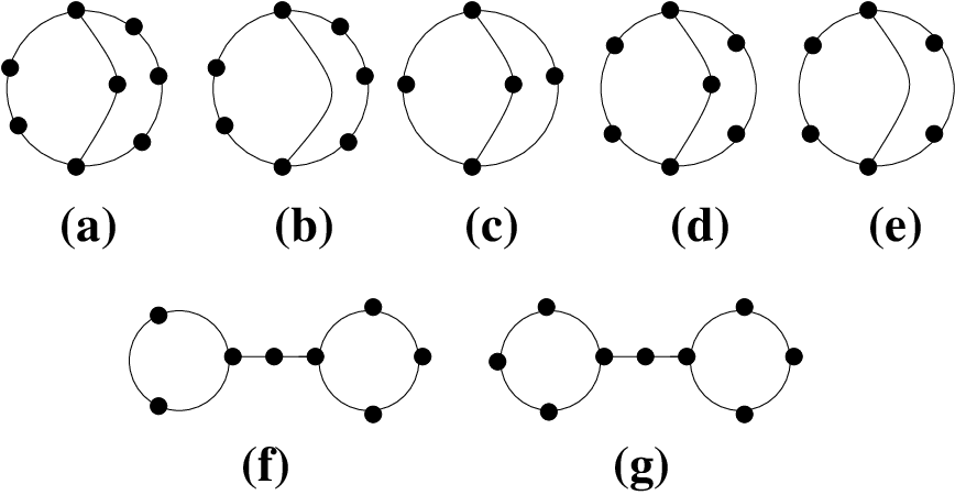
Refer to caption
Figure 6: The different basic smooth bicyclic graphs.

With the same notations as in Co70, denote by Pi​(z)P_{i}(z), respectively Qi​(z)Q_{i}(z), the generating functions of the number of partitions of an integer in ii parts, respectively in ii different parts. Let W^1¯​(z)\underline{\widehat{W}_{1}}(z) be the univariate EGF for smooth bicyclic graphs, then we have W^1¯​(z)=f⁡(P2​(z),P3​(z),Q2​(z),Q3​(z))\underline{\widehat{W}_{1}}(z)=f\big(P_{2}(z),P_{3}(z),Q_{2}(z),Q_{3}(z)\big), i.e.,

W^1¯​(z)=12​z2​(Q3​(z)+Q2​(z))⏟figures 6 (a), 6 (b)+112​z51−z3⏟6 (c)+14​(z41−z2+z5(1−z)​(1−z2)−z5(1−z3))⏟6 (d), 6 (e)+14​z6(1−z)2​(1−z2)⏟6 (f)+18​z5(1−z)​(1−z2)⏟6 (g).\begin{array}[]{cc}\underline{\widehat{W}_{1}}(z)=&\underbrace{\frac{1}{2}z^{2}(Q_{3}(z)+Q_{2}(z))}_{\mbox{figures \ref{basic_bicyclic} (a), \ref{basic_bicyclic} (b)}}+\underbrace{\frac{1}{12}\frac{z^{5}}{1-z^{3}}}_{\mbox{\ref{basic_bicyclic} (c)}}\\ &+\underbrace{\frac{1}{4}\left(\frac{z^{4}}{1-z^{2}}+\frac{z^{5}}{(1-z)(1-z^{2})}-\frac{z^{5}}{(1-z^{3})}\right)}_{\mbox{\ref{basic_bicyclic} (d), \ref{basic_bicyclic} (e)}}\\ &+\underbrace{\frac{1}{4}\frac{z^{6}}{(1-z)^{2}(1-z^{2})}}_{\mbox{\ref{basic_bicyclic} (f)}}+\underbrace{\frac{1}{8}\frac{z^{5}}{(1-z)(1-z^{2})}}_{\mbox{\ref{basic_bicyclic} (g)}}\,.\end{array} (12)

In formula (12) or equivalently W^1¯​(z)=z424​(6−z)(1−z)3\underline{\widehat{W}_{1}}(z)=\frac{z^{4}}{24}\frac{(6-z)}{(1-z)^{3}}, the denominator 1(1−z)3\frac{1}{(1-z)^{3}} denotes the fact that there is at most 33 arcs or 33 degrees of liberty of integer partitions of the vertices in a bicyclic graph. The same remark holds for the denominators 1(1−T⁡(z))3​k\frac{1}{(1-T(z))^{3k}} in Wright’s formulae Wr77 for all (k+1)(k+1)-cyclic connected labelled graphs. To get the whole EGF for bicyclic graphs, we have to substitute zz by T⁡(z)T(z) in W^1¯​(z)\underline{\widehat{W}_{1}}(z) in order to replace all (shrinked) vertices of the smooth graphs by labelled rooted trees. The form of these EGF takes its importance when studying the asymptotic behavior of random graphs or multigraphs with a given excess. In fact, the known expansion of the Cayley’s function, TT, at its singularity z=1ez=\frac{1}{e} is (see KP89; FO90; FS+)

T⁡(z)=1−2​δ+23​δ2−1136​2​δ3+⋯,(δ=1−e​z).T(z)=1-\sqrt{2}\delta+\frac{2}{3}{\delta}^{2}-\frac{11}{36}\sqrt{2}{\delta}^{3}+\cdots\,,\,\,(\delta=\sqrt{1-ez})\,. (13)

As the EGFs of multicyclic components can be expressed in terms of TT, the key point of their characteristics corresponds directly to the analytical properties of tree polynomial tn​(y)t_{n}(y) defined as follow

1(1−T⁡(z))y=∑n≥0tn​(y)​znn!.\frac{1}{(1-T(z))^{y}}=\sum_{n\geq 0}t_{n}(y)\frac{z^{n}}{n!}\,. (14)

(tn​(y)t_{n}(y) is a polynomial of degree nn in yy.) Knuth and Pittel KP89 studied their properties. For fixed yy as n→∞n\rightarrow\infty, we have (see (KP89, lemma 2))

tn​(y)=2​π​n(n−1/2+y/2)2y/2​Γ​(y/2)+O⁡(nn−1+y/2).t_{n}(y)=\frac{\sqrt{2\pi}n^{(n-1/2+y/2)}}{2^{y/2}\Gamma(y/2)}+O(n^{n-1+y/2})\,. (15)

This equation tells us that in the EGF, W^1\widehat{W}_{1} of bicyclic graphs, expressed here as a sum of powers of 1/(1−T⁡(z))1/(1-T(z))

W^1​(z)\displaystyle\widehat{W}_{1}(z) =\displaystyle= T​(z)424​(6−T⁡(z))(1−T⁡(z))3\displaystyle\frac{T(z)^{4}}{24}\frac{(6-T(z))}{(1-T(z))^{3}} (16)
=\displaystyle= 524​1(1−T⁡(z))3−1924​1(1−T⁡(z))2+⋯,\displaystyle\frac{5}{24}\frac{1}{(1-T(z))^{3}}-\frac{19}{24}\frac{1}{(1-T(z))^{2}}+\cdots\,, (17)

only the coefficient 524\frac{5}{24} of tn​(3)t_{n}(3) is asymptotically significant.

4 Functional equation for ξ\xi-free graphs/multigraphs and the forms of their EGFs

4.1 Differential recurrence for ξ\xi-free components

EGFs of triangle-free unicyclic components can be easily obtained when avoiding cycle of length 33 in the general formulae for unicyclic graphs (10), resp. multigraphs (11). Denote respectively by W0,C3W_{0,C_{3}} and W^0,C3\widehat{W}_{0,C_{3}} the EGFs for unicyclic multigraphs and graphs without triangle (C3C_{3}), we have

W0,C3​(z)=12​ln⁡11−T⁡(z)−T​(z)36,W_{0,C_{3}}(z)=\frac{1}{2}\ln{\frac{1}{1-T(z)}}-\frac{T(z)^{3}}{6}\,, (18)
W^0,C3​(z)=12​ln⁡11−T⁡(z)−T⁡(z)2−T​(z)24−T​(z)36.\widehat{W}_{0,C_{3}}(z)=\frac{1}{2}\ln{\frac{1}{1-T(z)}}-\frac{T(z)}{2}-\frac{T(z)^{2}}{4}-\frac{T(z)^{3}}{6}\,. (19)

Enumerating components of higher cyclic order without triangle is much more difficult. However, we have the following lemma:

Lemma 7

For all i≥−1i\geq-1, denote by W^i,C3\widehat{W}_{i,C_{3}} the EGF for triangle-free (i+1)(i+1)-cyclic graphs. Let S^i,C3\widehat{S}_{i,C_{3}} and J^i,C3\widehat{J}_{i,C_{3}} be the EGFs described as in definition 4. Then, the bivariate EGFs W^k+1,C3\widehat{W}_{k+1,C_{3}}, S^k+1,C3\widehat{S}_{k+1,C_{3}}, J^k+1,C3\widehat{J}_{k+1,C_{3}} and W^p,C3\widehat{W}_{p,C_{3}} for −1≤p≤k-1\leq p\leq k are related by the differential recurrence:

ϑw​W^k+1,C3\displaystyle\vartheta_{w}\widehat{W}_{k+1,C_{3}}\,\,\, +\displaystyle+   3​S^k+1,C3+J^k+1,C3=w⁡(ϑz2−ϑz2−ϑw)​W^k,C3\displaystyle\,\,3\widehat{S}_{k+1,C_{3}}\,\,+\,\,\widehat{J}_{k+1,C_{3}}\,\,=\,\,\,\,w\Big(\frac{{\vartheta_{z}}^{2}-\vartheta_{z}}{2}-\vartheta_{w}\Big)\widehat{W}_{k,C_{3}} (20)
+\displaystyle+ w⁡(∑−1≤p≤q≤k+1,p+q=k11+δp,q​(ϑz​W^p,C3)​(ϑz​W^q,C3))\displaystyle\,\,w\left(\sum_{-1\leq p\leq q\leq k+1,\,p+q=k}\frac{1}{1+\delta_{p,q}}(\vartheta_{z}\widehat{W}_{p,C_{3}})(\vartheta_{z}\widehat{W}_{q,C_{3}})\right)\, (21)

where δp,q=1\delta_{p,q}=1 iff p=qp=q, otherwise δp,q=0\delta_{p,q}=0. Similarly, we have for multigraphs (with the same parameters):

ϑw​Wk+1,C3\displaystyle\vartheta_{w}{W_{k+1,C_{3}}}\,\,\, +\displaystyle+   3​Sk+1,C3+Jk+1,C3=w⁡(ϑz22​Wk,C3)\displaystyle\,\,3{S_{k+1,C_{3}}}\,\,+\,\,{J_{k+1,C_{3}}}\,\,=\,\,\,\,w\Big(\frac{{\vartheta_{z}}^{2}}{2}{W_{k,C_{3}}}\Big) (22)
+\displaystyle+ w⁡(∑−1≤p≤q≤k+1,p+q=k11+δp,q​(ϑz​Wp,C3)​(ϑz​Wq,C3)).\displaystyle\,\,w\left(\sum_{-1\leq p\leq q\leq k+1,\,p+q=k}\frac{1}{1+\delta_{p,q}}(\vartheta_{z}{W_{p,C_{3}}})(\vartheta_{z}{W_{q,C_{3}}})\right)\,. (23)

Proof. There are two ways to obtain a (k+2)(k+2)-cyclic component from components of lower cyclic order, which are in the right part of (21) and are assumed to be triangle-free. For multigraphs, we have to employ the combinatorial operation ϑz22\frac{{\vartheta_{z}}^{2}}{2}.

First of all, consider a triangle-free (k+1)(k+1)-cyclic component. To add a new edge to this component, we have to choose two vertices, different and already not adjacent for graphs, and not necessarily different for multigraphs. For graphs, the combinatorial operator used to choose two different vertices is ϑz2−ϑz2\frac{{\vartheta_{z}}^{2}-\vartheta_{z}}{2}. Then, we have to avoid the adjacent vertices by means of the operator −ϑw-\vartheta_{w} (see (JKLP93, Section 10) or GJ83 for the use of marking and pointing). If the new (k+2)(k+2)-cyclic component contains a triangle, the triangle can only occur in the following cases:

  • 1.

    The new edge creates exactly a triangle. In this case, the last added edge is necessarily one of the 33 edges of the new triangle.

  • 2.

    The last edge creates many triangles but necessarily juxtaposed as defined above (definition 2), and in this latter case, the last edge is necessarily the one which is shared between all the occurrences of triangle.

Thus, the left side of (21), resp. of (23), distinguishes the last added edge in the new (k+2)(k+2)-cyclic component.

Next, a (k+2)(k+2)-cyclic triangle-free component can be built when creating an edge between a (p+1)(p+1)-cyclic and a (q+1)(q+1)-cyclic triangle-free components such that p+q=kp+q=k and −1≤p≤q≤k+1-1\leq p\leq q\leq k+1 (note that the case p=−1p=-1 and q=k+1q=k+1 corresponds to the case where a tree is attached to a (k+1)(k+1)-cyclic triangle-free component). This construction is done by choosing one vertex belonging to the (p+1)(p+1)-cyclic component and another vertex from the (q+1)(q+1)-cyclic component. A symmetry factor, 12!\frac{1}{2!}, occurs when p=qp=q.

The right side of (21) simply reflects the constructions used to build a (k+2)(k+2)-cyclic connected graph In (23), the term ϑz22​Wk,C3\frac{{\vartheta_{z}}^{2}}{2}{W_{k,C_{3}}} represents all (k+1)(k+1)-cyclic multigraphs with an ordered pair ⟨x,y⟩\langle x,y\rangle of marked vertices (see also (JKLP93, Sect. 4, Eq. (4.2) and following)). ∎

When considering a finite set ξ\xi of forbidden configurations, we have the following generalization of lemma 7:

Lemma 8

Suppose that ξ={H1,⋯,Hp}\xi=\{H_{1},\,\cdots,H_{p}\}, |ξ|<∞|\xi|<\infty. Let W^k+1,ξ\widehat{W}_{k+1,\xi}, S^k+1,Hi\widehat{S}_{k+1,H_{i}}, J^k+1,ξ\widehat{J}_{k+1,\xi} and W^k+1,ξ\widehat{W}_{k+1,\xi} be the EGFs defined as in above (definition 4). Let ρs\rho_{s} be the finite set of all ss-juxtapositions of member(s) of ξ\xi and denote by e⁡(Hi)e(H_{i}) the number of edges of HiH_{i}. Then, we have for graphs

ϑw​W^k+1,ξ\displaystyle\vartheta_{w}\widehat{W}_{k+1,\xi}\,\,\, +\displaystyle+ ∑Hi∈ξe⁡(Hi)​S^k+1,Hi+J^k+1,ξ=w⁡(ϑz2−ϑz2−ϑw)​W^k,ξ\displaystyle\,\,\sum_{H_{i}\in\xi}e(H_{i})\widehat{S}_{k+1,H_{i}}\,\,+\,\,\widehat{J}_{k+1,\xi}\,\,=\,\,\,\,w\Big(\frac{{\vartheta_{z}}^{2}-\vartheta_{z}}{2}-\vartheta_{w}\Big)\widehat{W}_{k,\xi} (24)
+\displaystyle+ w⁡(∑−1≤p≤q≤k+1,p+q=k11+δp,q​(ϑz​W^p,ξ)​(ϑz​W^q,ξ)).\displaystyle\,\,w\left(\sum_{-1\leq p\leq q\leq k+1,\,p+q=k}\frac{1}{1+\delta_{p,q}}(\vartheta_{z}\widehat{W}_{p,\xi})(\vartheta_{z}\widehat{W}_{q,\xi})\right)\,. (25)

For the EGFs of connected ξ\xi-free multigraphs, we have

ϑw​Wk+1,ξ\displaystyle\vartheta_{w}{W_{k+1,\xi}}\,\,\, +\displaystyle+ ∑Hi∈ξe⁡(Hi)​Sk+1,Hi+Jk+1,ξ=w⁡(ϑz22​Wk,ξ)+\displaystyle\,\,\sum_{H_{i}\in\xi}e(H_{i}){S_{k+1,H_{i}}}\,\,+\,\,J_{k+1,\xi}\,\,=\,\,\,\,w\Big(\frac{{\vartheta_{z}}^{2}}{2}{W_{k,\xi}}\Big)\,\,+ (26)
w⁡(∑−1≤p≤q≤k+1,p+q=k11+δp,q​(ϑz​Wp,ξ)​(ϑz​Wq,ξ)).\displaystyle\,\,w\left(\sum_{-1\leq p\leq q\leq k+1,\,p+q=k}\frac{1}{1+\delta_{p,q}}(\vartheta_{z}{W_{p,\xi}})(\vartheta_{z}{W_{q,\xi}})\right)\,. (27)

(25) and (27) are simply generalization of (21) and (23).

4.2 Bicyclic components without triangle

EGFs for respectively bicyclic graphs with one triangle and with exactly one juxtaposition of triangles can be obtained using the method developed in section 3, with the help of figures 8 and 8.

Remark 9

Since Wright’s reduction method11 1 the second method in Wr77, see also the proof of lemma 15 in §4.4 suggests us to work with labelled smooth components, figures such as 8 and 8 represent the situation after smoothing. Also for any family ℱk\mathcal{F}_{k} of (k+1)(k+1)-cyclic components with EGF Fk​(z)F_{k}(z), the EGF of smooth species of ℱk\mathcal{F}_{k} is simply obtained by means of substitutions of all occurrences of T⁡(z)T(z) in Fk​(z)F_{k}(z) by zz. Conversely, if Fk¯​(z)\underline{F_{k}}(z) is the EGF of smooth species of ℱk\mathcal{F}_{k}, then Fk​(z)=Fk¯​(T⁡(z))F_{k}(z)=\underline{F_{k}}(T(z)) gives the EGF associated to the whole family ℱk\mathcal{F}_{k}.

Remark 10

Since all EGFs we deal with can be expressed in terms of T⁡(z)T(z) in the univariate case, and of ww and T⁡(w​z)T(wz) in the bivariate case, we assume that T≡T⁡(z)T\equiv T(z) to express univariate EGFs. In the case of bivariate EGFs, we let T≡T⁡(w​z)T\equiv T(wz). These notations should not induce ambiguity to the reader who can read the meaning within the context.

The following figures can be used to compute the EGFs S^1,C3\widehat{S}_{1,C_{3}} and J^1,C3\widehat{J}_{1,C_{3}}

Refer to caption
Figure 7: Smooth bicyclic graphs with one occurrence of triangle.
Refer to caption
Figure 8: Smooth bicyclic graph with a 11-juxtaposition of 2 triangles.

Using similar techniques as for (12) with the help of the previous figures, we have for S^1,C3¯\underline{\widehat{S}_{1,C_{3}}} and J^1,C3¯\underline{\widehat{J}_{1,C_{3}}}

S^1,C3¯​(z)=12​z5​11−z⏟figure 8 (b)+z64​1(1−z)2⏟figure 8 (a)\begin{array}[]{cc}\underline{\widehat{S}_{1,C_{3}}}(z)=&\underbrace{\frac{1}{2}z^{5}\frac{1}{1-z}}_{\mbox{figure \ref{FIG:SMOOTH_S1} (b)}}+\underbrace{\frac{z^{6}}{4}\frac{1}{(1-z)^{2}}}_{\mbox{figure \ref{FIG:SMOOTH_S1} (a)}}\end{array} (28)

and

J^1,C3¯​(z)=z44.\underline{\widehat{J}_{1,C_{3}}}(z)=\frac{z^{4}}{4}\,. (29)

Again, to obtain the whole EGFs we have to substitute zz by T≡T⁡(z)T\equiv T(z), replacing all shrinked vertices of the smooth graphs by labelled rooted trees.

S^1,C3​(z)=T54​(2−T)(1−T)2,J^1,C3​(z)=T44.\widehat{S}_{1,C_{3}}(z)=\frac{T^{5}}{4}\frac{(2-T)}{(1-T)^{2}}\,,\,\,\widehat{J}_{1,C_{3}}(z)=\frac{T^{4}}{4}\,. (30)

Thus, using (30) and (21) we have

W^1,C3​(z)=T524​(2+6​T−3​T2)(1−T)3.\widehat{W}_{1,C_{3}}(z)=\frac{T^{5}}{24}\frac{(2+6T-3T^{2})}{(1-T)^{3}}\,. (31)

We know from (15) that the decomposition of formula such as (31) into sums of powers of 11−T\frac{1}{1-T}, are useful in order to study the asymptotic behavior of the number of such objects. We have

W^1,C3​(z)=∑n≥0(524​tn​(3)−2524​tn​(2)+4724​tn​(1)−3524−524​tn​(−1)CLOSEOPEN+2524​tn​(−2)−58​tn​(−3)+18​tn​(−4))​znn!.\begin{array}[]{ccc}\widehat{W}_{1,C_{3}}(z)&=&\sum_{n\geq 0}\Big(\frac{5}{24}t_{n}(3)-\frac{25}{24}t_{n}(2)+\frac{47}{24}t_{n}(1)-\frac{35}{24}-\frac{5}{24}t_{n}(-1)\\ &&+\frac{25}{24}t_{n}(-2)-\frac{5}{8}t_{n}(-3)+\frac{1}{8}t_{n}(-4)\Big)\frac{z^{n}}{n!}\,.\end{array} (32)

In order to enumerate the first multicyclic ξ\xi-free components for general ξ\xi, we introduce some more techniques in the next paragraphs.

4.3 General techniques for first multicyclic components and instantiations

In this paragraph, we give methods that can be applied to enumerate first low-order cyclic components, i.e., with excess 11 and 22 for a forbidden pp-gon and in general for an excess up to l+1l+1 and l+2l+2 for all forbidden components of excess ll. For e.g., the EGF of C3C_{3}-free tricyclic graphs are given as instantiation of these methods and follows the formula (31) given above. Also, we will see later that these techniques are useful to obtain the forms of the EGFs W^k,ξ\widehat{W}_{k,\xi} and Wk,ξW_{k,\xi} by induction (see §4.4). We consider here only connected graphs with exactly one occurrence of HH since if H′H^{{}^{\prime}} represents any juxtaposition of HH, we can work directly in the same manner with a single occurrence of H′H^{{}^{\prime}}.

First of all, we have to prune recursively all vertices of degree 11. The obtained graphs are smooth. We can subdivide these graphs containing an occurrence of HH in 3 types: types (a) and (b) are such as those represented by figure 8 and type (c) is as in the figure 9 below where HH represents a triangle.

Refer to caption
Figure 9:

The first two types (a) and (b) of figure 8 can be described as follows:

  • ∙\bullet

    (a) represents the concatenation of two components HH and FF (respectively non HH-free and HH-free) by a common vertex or more generally by a path between the two components. In the figure, HH is simply a triangle. Note that a cutpoint (a vertex whose removal increases the number of connected components) belongs to the triangle after the recursive deletions of vertices of degree 11. This is referred here as a serial composition of components.

  • ∙\bullet

    (b) is the concatenation of the same components but by a common edge. This construction is referred as a parallel composition of components.

  • ∙\bullet

    Figure 9 (c) represents components which are not in figure 8 (a) nor in figure 8 (b).

4.3.1 The serial composition or concatenation by a vertex

Since a graph with one cutpoint belonging to a forbidden configuration may be considered to be rooted at this cutpoint, the number of connected graphs with one cutpoint can be expressed in terms of the EGFs of the different subgraphs rooted at the same cutpoint (cf. HP73 or Selkow). This construction may be interpreted combinatorially as follows.

Lemma 11

Let ℱ\mathcal{F} be a family of connected HH-free graph. Denote by F¯\underline{F} the EGF of the graphs obtained when smoothing a graph of ℱ\mathcal{F}. Let A1A_{1} be the EGF of connected graphs containing possibly many copies of HH and obtained as the concatenation of graphs of ℱ\mathcal{F} and of HH by a vertex belonging to HH. Then, A1A_{1} satisfies

A1⪯[1z(z∂∂zF¯(z))(z∂∂zH(z))]|z=T(z)A_{1}\preceq{\left[\frac{1}{z}\,\,\left(z\frac{\partial}{\partial z}\underline{F}(z)\right)\,\left(z\frac{\partial}{\partial z}H(z)\right)\right]}_{|z=T(z)} (33)

and let A2A_{2} be the EGF of all connected graphs obtained when allowing a path starting at a vertex belonging to HH and joining any graph of ℱ\mathcal{F}. A2A_{2} satisfies

A2⪯[1z(11−z)(z∂∂zF¯(z))(z∂∂zH(z))]|z=T(z).A_{2}\preceq{\left[\frac{1}{z}\,\left(\frac{1}{1-z}\right)\,\left(z\frac{\partial}{\partial z}\underline{F}(z)\right)\,\left(z\frac{\partial}{\partial z}H(z)\right)\right]}_{|z=T(z)}\,. (34)

In (33) and (34), equalities hold when HH is two-connected.

Proof. Recall that for two EGFs AA and BB, A⪯BA\preceq B means that ∀n,[zn]​A​(z)≤[zn]​B​(z)\forall n,\,\left[z^{n}\right]A(z)\leq\left[z^{n}\right]B(z) (cf. remark 6). First, let us consider the case where HH is two-connected. In this case, the concatenation of HH with a graph of ℱ\mathcal{F}, by a vertex of HH, leads to a graph with a single copy of HH in the resulting graph. Thus, the fact that there is exactly one occurrence of copy of HH in the concatenation insures the uniqueness of the decomposition into two graphs such that one belongs to ℱ\mathcal{F} and the other is (necessarily) HH. The lemma is a combination of the approach presented in Selkow and Wright’s reduction method Wr77. We have to introduce a factor 1z\frac{1}{z} to relabel the common cutpoint considered here as shared between the smooth components. ϑz​F¯​(z)=z​∂∂z​F¯​(z)\vartheta_{z}\underline{F}(z)=z\frac{\partial}{\partial z}\underline{F}(z) and ϑz​H​(z)=z​∂∂z​H​(z)\vartheta_{z}H(z)=z\frac{\partial}{\partial z}H(z) are used to distinguish the vertex to be shared between pruned components of ℱ\mathcal{F} and of HH. In (34) to represent a possible path, we insert the term 11−z\frac{1}{1-z} i.e., a sequence of vertices of degree 2 except the two extremal nodes, between the two sides. When substituting zz by T⁡(z)T(z), we reverse the vertexectomy process starting with a smooth graph and sprout rooted trees from each node. Hence, in the case where HH is two-connected, we have the equalities in (33) and (34). The situation changes a bit for more general configurations. Typically, we can have concatenations of HH and graphs of ℱ\mathcal{F} which can lead to a new graph with two (or more) occurrences of HH. This is the case depicted by figure 10

Refer to caption
Figure 10: Serial composition with symmetric factor 12\frac{1}{2}.

where HH is made with a triangle and a square attached by a vertex and the graph of ℱ\mathcal{F} is simply a triangle. In this special case, we just have to introduce a symmetry factor 12!\frac{1}{2!} and then the upper bound of (33) is valid. In fact, the upper bound enumerates graphs where the concatenation such as the one obtained in figure 10 are counted twice or more. ∎

4.3.2 The parallel composition or concatenation by an edge

Graphs of the type represented by the figure 8 (b) can be enumerated in a very close way.

Lemma 12

Let ℱ\mathcal{F} and F¯\underline{F} be defined as in lemma 11 above. Let BB be the EGF associated to the graphs containing copies of HH and obtained as the concatenation of two graphs of ℱ\mathcal{F} and of HH sharing a common edge. BB satisfies

B⪯[2w​z2(w∂∂wF¯(w,z))(w∂∂wH(w,z))]|wz=T(wz).B\preceq{\left[\frac{2}{wz^{2}}\,\,\left(w\frac{\partial}{\partial w}\underline{F}(w,z)\right)\,\,\left(w\frac{\partial}{\partial w}H(w,z)\right)\right]}_{|wz=T(wz)}\,. (35)

Proof. The formula (35) differs slightly from the one in (34). The factor 2w​z2\frac{2}{wz^{2}} comes from the fact that we have here, as in the figure 8 (b), a common edge which is defined by his two common vertices and can be seen as a root-edge. A graph such as those represented by the figure 8 (b) can be considered as pendant to this edge. Also, we have the equality whenever HH is two-connected. Otherwise symmetries can arise but the upper bound of (35) remains valid for the same reasons as for (33) and (34). ∎

Unfortunately, equation likes (25) of lemma 8 are much easier to propose than to really solve. However, we can derive the EGF of the first multicyclic HH-free components by applying the techniques presented above.

4.3.3 The example of triangle-free graphs

The EGFs of unicyclic and bicyclic graphs without triangles are given by formulae (19) and (31). For graphs having 22 excesses, the removal of all edges and vertices by the Wright’s reduction method leads to the set of graphs represented by figure 11 for graphs containing 11 triangle and figure 12 for graphs with a juxtaposition of triangles.

Refer to caption
Figure 11: Basic tricyclic graphs with exactly one triangle. The subgraph in grey represent bicyclic triangle-free components.

As before, given a family ℱ\mathcal{F} of graphs, we denote by F¯\underline{F} the EGF of smooth elements of ℱ\mathcal{F}, i.e., graphs without endvertices (vertices of degree 11). The bivariate EGF of bicyclic triangle-free smooth graphs, W^1,C3¯\underline{\widehat{W}_{1,C_{3}}} is obtained from (31), namely

W^1,C3¯​(w,z)=w​w5​z524​(2+6​w​z−3​w2​z2)(1−w​z)3\underline{\widehat{W}_{1,C_{3}}}(w,z)=w\frac{w^{5}z^{5}}{24}\frac{(2+6wz-3w^{2}z^{2})}{(1-wz)^{3}} (36)

Note that ϑw​C3​(w,z)=ϑz​C3​(w,z)=w3​z32\vartheta_{w}C_{3}(w,z)=\vartheta_{z}C_{3}(w,z)=\frac{w^{3}z^{3}}{2}. Thus, the application of the lemmas 11 and 12 to the smooth graphs depicted by figures 11 (a) and 11 (b) gives

w3​z22​(1−w​z)​ϑz​(W^1,C3¯​(w,z))+w2​z​ϑw​(W^1,C3¯​(w,z)).{\frac{w^{3}z^{2}}{2(1-wz)}\,\,\vartheta_{z}\big(\underline{\widehat{W}_{1,C_{3}}}(w,z)\big)+w^{2}z\,\,\vartheta_{w}\big(\underline{\widehat{W}_{1,C_{3}}}(w,z)\big)}\,. (37)

Similarly, we have for smooth graphs represented by the figure 11 (d)

1z⁡(1−w​z)​(2w​z2​(ϑw​W^0,C3¯​(w,z))​(w3​z32))​(ϑz​W^0,C3¯​(w,z)){\frac{1}{z(1-wz)}\Big(\frac{2}{wz^{2}}\,\big(\vartheta_{w}\underline{\widehat{W}_{0,C_{3}}}(w,z)\big)\,\big(\frac{w^{3}z^{3}}{2}\Big)\Big)\Big(\vartheta_{z}\underline{\widehat{W}_{0,C_{3}}}(w,z)\Big)} (38)

and for figure 11 (e), we find

2w​z2​(2w​z2​(w3​z32)​(ϑw​W^0,C3¯​(w,z))2).\frac{2}{wz^{2}}\left(\frac{2}{wz^{2}}\Big(\frac{w^{3}z^{3}}{2}\Big)\Big(\vartheta_{w}\underline{\widehat{W}_{0,C_{3}}}(w,z)\Big)^{2}\right)\,. (39)

A simple way to enumerate the smooth graphs represented by the figure 11 (c) is to consider that the three paths between the triangle and the vertex vv are symmetric. Taking into account the fact that only one of these three paths can be reduced to a simple edge (to avoid another triangle), we have the following EGF associated to these smooth graphs

z73!​(1−z)3+z62!​(1−z)2.\frac{z^{7}}{3!(1-z)^{3}}+\frac{z^{6}}{2!(1-z)^{2}}\,. (40)

In total, the bivariate EGF for all graphs such that smooth species are depicted by the figures 11 (c), 11 (d) and 11 (e) is given by

w2​T66​(3−2​T)(1−T)3+w2​T72​(1−T)2+w2​T84​(1−T)3.w^{2}\frac{T^{6}}{6}\frac{(3-2T)}{(1-T)^{3}}+\frac{w^{2}T^{7}}{2(1-T)^{2}}+\frac{w^{2}T^{8}}{4(1-T)^{3}}\,. (41)

Summing (37) and (41), one can deduce the bivariate EGF for tricyclic graphs containing exactly a triangle

S^2,C3​(w,z)=w2​T648​(48+18​T−140​T2+119​T3−30​T4)(1−T)5.\widehat{S}_{2,C_{3}}(w,z)=\frac{w^{2}T^{6}}{48}\frac{(48+18T-140T^{2}+119T^{3}-30T^{4})}{(1-T)^{5}}\,. (42)

We turn now to the enumeration of tricyclic graphs with one occurrence of juxtaposition of triangles. The figure 12 represents the 2-excess smooth graphs with juxtapositions of triangles.

Refer to caption
Figure 12: Basic tricyclic graphs with juxtapositions of triangles.

We observe that figures 12 (b) and 12 (c) can be handled with the techniques of lemma 12 using the EGF W^0,C3¯\underline{\widehat{W}_{0,C_{3}}} and w5​z42!​2!\frac{w^{5}z^{4}}{2!2!} (which is the EGF of the smooth juxtaposition of 22 triangles). Similarly, we can use lemma 11 for the figures 12 (d) and 12 (e). The EGF associated to the smooth graph of figure 12 (a) is simply w7​z52!​3!\frac{w^{7}z^{5}}{2!3!}, and the one for smooth graphs depicted by the figure 12 (f) is w7​z54​(1−w​z)\frac{w^{7}z^{5}}{4(1-wz)}. In fact, graphs such as the one drawn in figure 12 (f) can be obtained by replacing an edge of the complete graph K4K_{4} with a path of length at least 22. The EGF that corresponds to the figure 12 is then

J^2,C3¯​(w,z)=wz⁡(1−w​z)​ϑz​(w5​z44)​ϑz​(W^0,C3¯​(w,z))\displaystyle\underline{\widehat{J}_{2,C_{3}}}(w,z)=\frac{w}{z(1-wz)}\vartheta_{z}\big(\frac{w^{5}z^{4}}{4}\big)\vartheta_{z}\big(\underline{\widehat{W}_{0,C_{3}}}(w,z)\big) (43)
+2w​z2​ϑw​(w5​z44)​ϑw​(W^0,C3¯​(w,z))+w2​(w​z)52!​3!+w2​(w​z)54​(1−w​z).\displaystyle+\frac{2}{wz^{2}}\vartheta_{w}\big(\frac{w^{5}z^{4}}{4}\big)\vartheta_{w}\big(\underline{\widehat{W}_{0,C_{3}}}(w,z)\big)+{w^{2}\frac{(wz)^{5}}{2!3!}}+{w^{2}\frac{(wz)^{5}}{4(1-wz)}}\,. (44)

Thus, the bivariate EGF of tricyclic graphs containing exactly a juxtaposition of triangles is

J^2,C3​(w,z)=w2​T56​(2+5​T−4​T2)(1−T)2.\widehat{J}_{2,C_{3}}(w,z)=\frac{w^{2}T^{5}}{6}\frac{(2+5T-4T^{2})}{(1-T)^{2}}\,. (45)

The bivariate EGF of tricyclic triangle-free graphs is then obtained using (42), (45) and (21), namely,

W^2,C3​(w,z)=w2​T648​(7+36​T−18​T2−40​T3+40​T4−10​T5)(1−T)6.\widehat{W}_{2,C_{3}}(w,z)=w^{2}\frac{T^{6}}{48}\frac{(7+36T-18T^{2}-40T^{3}+40T^{4}-10T^{5})}{(1-T)^{6}}\,. (46)

4.4 General forms of the EGFs of ξ\xi-free components

Although lemmas 7 and 8 do not allow us to solve completely the problems of enumerating ξ\xi-free connected graphs with a given number of vertices and edges, the combination of these lemmas with subtle combinatorial constructions provides alternative solutions to get the general forms of the EGFs W^k,ξ\widehat{W}_{k,\xi} and Wk,ξ{W_{k,\xi}}. Recall the following theorem due to Wright

Theorem 13 (Wright 1977)

For k≥1k\geq 1, the EGFs, Wk^\widehat{W_{k}}, of (k+1)(k+1)-cyclic graphs can be expressed as a finite sum of powers of 11−T⁡(z)\frac{1}{1-T(z)} with rational coefficients and we have

W^k​(z)=bk(1−T⁡(z))3​k−ck(1−T⁡(z))3​k−1+∑2≤s≤3​k−2ωk,s(1−T⁡(z))s.\widehat{W}_{k}(z)=\frac{b_{k}}{(1-T(z))^{3k}}-\frac{c_{k}}{(1-T(z))^{3k-1}}+\sum_{2\leq s\leq 3k-2}\frac{\omega_{k,s}}{(1-T(z))^{s}}\,. (47)

The (bk)k≥1(b_{k})_{k\geq 1} are called the Wright’s constants of first order (also called Wright-Louchard-Takács constants, see for e.g. Sp97). b1=524b_{1}=\frac{5}{24} and for k≥1k\geq 1, bkb_{k} is defined recursively by

2​(k+1)​bk+1=3​k​(k+1)​bk+3​∑t=1k−1t⁡(k−t)​bt​bk−t.2(k+1)b_{k+1}=3k(k+1)b_{k}+3\sum_{t=1}^{k-1}t(k-t)b_{t}b_{k-t}\,. (48)

The (ck)k≥1(c_{k})_{k\geq 1} are the Wright’s constants of second order and are defined recursively, using (48), by c1=1924c_{1}=\frac{19}{24} and for k≥1k\geq 1

2​(3​k+2)​ck+1\displaystyle 2(3k+2)c_{k+1} =\displaystyle= 8​(k+1)​bk+1+3​k​bk+(3​k+2)​(3​k−1)​ck\displaystyle 8(k+1)b_{k+1}+3kb_{k}+(3k+2)(3k-1)c_{k} (49)
+\displaystyle+ 6​∑t=1k−1t⁡(3​k−3​t−1)​bt​ck−t.\displaystyle 6\sum_{t=1}^{k-1}t(3k-3t-1)b_{t}c_{k-t}\,. (50)

The proof of theorem 13 is an interesting combinatorial exercise involving essentially the pointing operators ϑw\vartheta_{w} and ϑz\vartheta_{z} (see Wr77; JKLP93). Note that formulae (47), (48) and (50) are obtained with Wright’s fundamental differential recurrence (well explained in (JKLP93, section 6)) and which is written here with the notations of this paper

ϑw​W^k+1\displaystyle\vartheta_{w}\widehat{W}_{k+1} =\displaystyle= w⁡(ϑz2−ϑz2−ϑw)​W^k\displaystyle\,\,\,\,w\Big(\frac{{\vartheta_{z}}^{2}-\vartheta_{z}}{2}-\vartheta_{w}\Big)\widehat{W}_{k} (51)
+\displaystyle+ w⁡(∑−1≤p≤q≤k+1,p+q=k11+δp,q​(ϑz​W^p)​(ϑz​W^q)).\displaystyle\,\,w\left(\sum_{-1\leq p\leq q\leq k+1,\,p+q=k}\frac{1}{1+\delta_{p,q}}(\vartheta_{z}\widehat{W}_{p})(\vartheta_{z}\widehat{W}_{q})\right)\,. (52)

For our connected (k+1)(k+1)-cyclic triangle-free graphs, we have the following existence theorem on the forms of their EGFs:

Theorem 14

There exists rational ωk,i(C3)\omega_{k,i}^{(C_{3})} such that for all k≥2k\geq 2, the univariate EGF, W^k,C3\widehat{W}_{k,C_{3}}, associated to (k+1)(k+1)-cyclic triangle-free graphs, is of the form:

W^k,C3​(z)=bk(1−T)3​k−ck(C3)(1−T)3​k−1+∑i≤3​k−2ωk,i(C3)(1−T)i\widehat{W}_{k,C_{3}}(z)=\frac{b_{k}}{(1-T)^{3k}}-\frac{c_{k}^{(C_{3})}}{(1-T)^{3k-1}}+\sum_{i\leq 3k-2}\frac{{\omega}_{k,i}^{(C_{3})}}{(1-T)^{i}} (53)

where T≡T⁡(z)T\equiv T(z), the summation is finite and the coefficients ck(C3)c_{k}^{(C_{3})} are defined, for all k≥1k\geq 1, by

r​l.c1(C3)=2524,ck+1(C3)=ck+1+32​k​bk.\begin{array}[]{\{}{rl}.&c_{1}^{(C_{3})}=\frac{25}{24}\,,\\ &c_{k+1}^{(C_{3})}=c_{k+1}+\frac{3}{2}kb_{k}\,.\end{array} (54)

Before proving theorem 14, the connected components with one occurrence of triangle are subdivided into 33 kinds of constructions, according to the degrees of the vertices of the unique triangle (after smoothing). Let us define these classifications. A smooth graph containing a triangle is of three kinds:

  • -

    exactly one vertex of the triangle is of degree ≥3\geq 3,

  • -

    exactly two vertices of the triangle are of degree ≥3\geq 3,

  • -

    the 33 vertices of the triangle are all of degree ≥3\geq 3.

Refer to caption
Figure 13: One vertex of the triangle is of degree ≥3\geq 3.
Refer to caption
Figure 14: Two vertices of the triangle are of degree ≥3\geq 3.
Refer to caption
Figure 15: Other smooth components.

Graphs whose situations after smoothing are depicted by figures 15 and 15 can be handled by the techniques of lemmas 11 and 12, and will be considered more precisely later. Note that in the figures, the right parts (in grey) of the constructions correspond to multicyclic structures without triangle. The lemma 15 gives the form of the EGF of the connected component with exactly one occurrence of triangle depicted by the figure 15.

Lemma 15

The EGF of (k+1)(k+1)-cyclic graphs containing one occurrence of triangle with all of its vertices of degree at least 33 has the following form

∑s≤3​k−3ϵk,s(1−T⁡(z))s\sum_{s\leq 3k-3}\frac{\epsilon_{k,s}}{(1-T(z))^{s}}\, (55)

where the summation is finite and the coefficients ϵk,s\epsilon_{k,s} are rational numbers.

Proof. Our idea is to apply Wright’s reduction method on our specific configuration. Since this method is known but is not that familiar, we repeat here the main steps. Suppose that we have a connected graph with kk edges more than vertices containing one triangle and suppose that the recursive suppressions of vertices of degree 11 lead to a graph of the type depicted by figure 15. That is, the obtained smooth graph has tt vertices of degree at least 22 and t+kt+k edges (here, tt is less that or equal to the number of vertices of the original graph). This way, we get a smooth graph with rr vertices of degree at least 33, r≤2​kr\leq 2k. These vertices of degree ≥3\geq 3 are called special vertices and let us color the edges of the triangle in order to distinguish them. The paths between these points, except the colored edges of the triangle, are of four kinds and we apply the following special operations on them (see (Wr77, Sect.  6)):

  • 1.

    An α\alpha-path begins and ends with the same special point and so must have at least two interior points. We elide all its interior points except two of them.

  • 2.

    A β\beta-path joins two different special vertices and we elide all its interior points.

  • 3.

    If two different special vertices are joined by more than one special path, at most one of these paths is reduced to a single edge which we call a δ−p​a​t​h\delta-path.

  • 4.

    The remaining paths, or all the paths if there is no δ\delta-path, are called γ\gamma-paths and for each γ\gamma-path, we elide all its interior points except one of them.

The obtained graph is called Wright’s basic graph. Denote respectively by aa, bb, cc and dd the number of α\alpha-, β\beta-, γ\gamma- and δ\delta- paths. Since each elision has removed exactly one edge and one vertex, the number of vertices of the basic graph is exactly r+2​a+cr+2a+c. Taking into account, the colored edges of the triangle and the operations made upon the special paths, the number of edges in the basic graph is r+2​a+c+k=3​a+b+2​c+d+3r+2a+c+k=3a+b+2c+d+3. Thus, we have a+b+c+d+3=r+k≤3​ka+b+c+d+3=r+k\leq 3k. We find

a+b+c≤3​k−3.a+b+c\leq 3k-3\,. (56)

To obtain any of the original graphs without vertices of degree 11, we distribute the previously t−r−2​a−ct-r-2a-c elided nodes on the α\alpha-, β\beta- and γ\gamma- paths. (56) gives us ideas on the number of ways to redistribute these points: suppose that f⁡(n)f(n) is the number of labelings of the (n,n+k)(n,n+k)-graphs which can produce the considered basic graph. Let F⁡(z)F(z) be their EGF:

F⁡(z)=∑nf⁡(n)​znn!.F(z)=\sum_{n}f(n)\frac{z^{n}}{n!}\,. (57)

To obtain each of the original (t,t+k)(t,t+k) graphs without endvertices, the distribution of the (t−r−2​a−c)(t-r-2a-c) nodes on the (a+b+c)(a+b+c) α\alpha-, β\beta- and γ\gamma-paths can be done in yy ways where yy is the number of partitions of (t−r−2​a−c)(t-r-2a-c) into (a+b+c)(a+b+c) parts. Relabel the obtained graph and replace the tt vertices with tt rooted and labelled trees. All the graphs are enumerated but they are not all different. In fact, they are enumerated gg times where gg is the order of the automorphisms of the current Wright’s basic graph. Thus, we have

g​F​(z)=∑ty​T​(z)t=T​(z)r+2​a+c(1−T⁡(z))a+b+c.gF(z)=\sum_{t}yT(z)^{t}=\frac{T(z)^{r+2a+c}}{(1-T(z))^{a+b+c}}\,. (58)

Summing over all the finitely many possible basic graphs, we obtain the lemma. ∎

Proof of theorem 14. Denote by (𝒫k,W^)({\mathcal{P}}_{k,\widehat{W}}), (𝒫k,S^)({\mathcal{P}}_{k,\widehat{S}}) and (𝒫k,J^)({\mathcal{P}}_{k,\widehat{J}}) the following properties:

  • ∙\bullet

    (𝒫k,W^)({\mathcal{P}}_{k,\widehat{W}}) : W^k,C3\widehat{W}_{k,C_{3}} is of the form given by the equation (53).

  • ∙\bullet

    (𝒫k,S^)({\mathcal{P}}_{k,\widehat{S}}) :
    If k=1k=1,

    S^1,C3​(z)=14​(1−T)2−1(1−T)−14​T4+14​T2+12​T+34\widehat{S}_{1,C_{3}}(z)=\frac{1}{4\,(1-T)^{2}}-\frac{1}{(1-T)}-\frac{1}{4}{T}^{4}+\frac{1}{4}{T}^{2}+\frac{1}{2}T+\frac{3}{4}\, (59)

    and for all k≥2k\geq 2, S^k,C​3\widehat{S}_{k,C3} is of the form

    S^k,C3​(z)=3​(k−1)​bk−12​(1−T⁡(z))3​k−1+∑i≤3​k−2σk,i(C3)(1−T⁡(z))i.\widehat{S}_{k,C_{3}}(z)=\frac{3(k-1)b_{k-1}}{2\,\big(1-T(z)\big)^{3k-1}}+\sum_{i\leq 3k-2}\frac{\sigma_{k,i}^{(C_{3})}}{\big(1-T(z)\big)^{i}}\,. (60)
  • ∙\bullet

    (𝒫k,J^)({\mathcal{P}}_{k,\widehat{J}}) :
    If k=1k=1

    J^1,C3​(z)=T44\widehat{J}_{1,C_{3}}(z)=\frac{T^{4}}{4}\, (61)

    and if k=2k=2, we have

    J^2,C3​(z)=12​(1−T)2−2(1−T)+32+T+T22−T42−2​T53.\widehat{J}_{2,C_{3}}(z)=\frac{1}{2(1-T)^{2}}-\frac{2}{(1-T)}+\frac{3}{2}+T+\frac{T^{2}}{2}-\frac{T^{4}}{2}-\frac{2T^{5}}{3}\,. (62)

    For all k≥3k\geq 3, J^k,C3\widehat{J}_{k,C_{3}} is of the form

    J^k,C3​(z)=3​(k−2)​bk−2(1−T⁡(z))3​k−4+∑i≤3​k−5υk,i(C3)(1−T⁡(z))i.\widehat{J}_{k,C_{3}}(z)=\frac{3(k-2)b_{k-2}}{\big(1-T(z)\big)^{3k-4}}+\sum_{i\leq 3k-5}\frac{\upsilon_{k,i}^{(C_{3})}}{\big(1-T(z)\big)^{i}}\,. (63)

where the coefficients (ωk,i(C3))(\omega_{k,i}^{(C_{3})}), (σk,i(C3))(\sigma_{k,i}^{(C_{3})}) and (υk,i(C3))(\upsilon_{k,i}^{(C_{3})}) are rational numbers and the summations in (53), (60) and (63) are finite.

We will show by induction on kk, that for all k≥1k\geq 1, the properties (𝒫k,W^)({\mathcal{P}}_{k,\widehat{W}}), (𝒫k,S^)({\mathcal{P}}_{k,\widehat{S}}) and (𝒫k,J^)({\mathcal{P}}_{k,\widehat{J}}) described above are simultaneously verified. To do this, we have (𝒫1,W^)({\mathcal{P}}_{1,\widehat{W}}), (𝒫1,S^)({\mathcal{P}}_{1,\widehat{S}}), (𝒫1,J^)({\mathcal{P}}_{1,\widehat{J}}) and (𝒫2,J^)({\mathcal{P}}_{2,\widehat{J}}) and we have to check that if (𝒫i,W^)({\mathcal{P}}_{i,\widehat{W}}), (𝒫i,S^)({\mathcal{P}}_{i,\widehat{S}}) and (𝒫i,J^)({\mathcal{P}}_{i,\widehat{J}}) are true for all ii such that 1≤i≤k−11\leq i\leq k-1 then (𝒫k,W^)({\mathcal{P}}_{k,\widehat{W}}), (𝒫k,S^)({\mathcal{P}}_{k,\widehat{S}}) and (𝒫k,J^)({\mathcal{P}}_{k,\widehat{J}}) are also satisfied. Note that due to the presence of the factor (k−1)(k-1) in (60), resp. (k−2)(k-2) in (63), we have to give S^1,C3\widehat{S}_{1,C_{3}}, J^1,C3\widehat{J}_{1,C_{3}} and J^2,C3\widehat{J}_{2,C_{3}}. Rewriting (46) and (42) as sums of powers of 11−T\frac{1}{1-T}, we have

W^2,C3​(z)=516​(1−T)6−53​(1−T)5+16748​(1−T)4−9124​(1−T)3\displaystyle\widehat{W}_{2,C_{3}}(z)=\frac{5}{16(1-T)^{6}}-\frac{5}{3(1-T)^{5}}+\frac{167}{48(1-T)^{4}}-\frac{91}{24(1-T)^{3}} (64)
+5516​(1−T)2−358​(1−T)+12548+17​T12+11​T224−5​T324−5​T412−5​T524,\displaystyle+\frac{55}{16(1-T)^{2}}-\frac{35}{8(1-T)}+\frac{125}{48}+\frac{17T}{12}+\frac{11T^{2}}{24}-\frac{5T^{3}}{24}-\frac{5T^{4}}{12}-\frac{5T^{5}}{24}\,, (65)
S^2,C3​(z)=516​(1−T)5−6548​(1−T)4+73​(1−T)3−7324​(1−T)2\displaystyle\widehat{S}_{2,C_{3}}(z)=\frac{5}{16(1-T)^{5}}-\frac{65}{48(1-T)^{4}}+\frac{7}{3(1-T)^{3}}-\frac{73}{24(1-T)^{2}} (66)
+6112​(1−T)−103−103​T48−53​T248−5​T348+31​T448+5​T58.\displaystyle+\frac{61}{12(1-T)}-\frac{10}{3}-\frac{103T}{48}-\frac{53T^{2}}{48}-\frac{5T^{3}}{48}+\frac{31T^{4}}{48}+\frac{5T^{5}}{8}\,. (67)

Thus, S^2,C3​(z)\widehat{S}_{2,C_{3}}(z), J^2,C3​(z)\widehat{J}_{2,C_{3}}(z), and W^2,C3​(z)\widehat{W}_{2,C_{3}}(z) can be formulated as finite sums of power of 1(1−T)\frac{1}{(1-T)} and properties (𝒫2,W^)({\mathcal{P}}_{2,\widehat{W}}), (𝒫2,S^)({\mathcal{P}}_{2,\widehat{S}}) and (𝒫2,J^)({\mathcal{P}}_{2,\widehat{J}}) are satisfied. Note that we let b0=12b_{0}=\frac{1}{2}, due to the fact that ϑz​W^0,C3​(z)=12​T4(1−T)\vartheta_{z}\,\widehat{W}_{0,C_{3}}(z)=\frac{1}{2}\,\frac{T^{4}}{(1-T)}. Now, suppose that (𝒫i,W^)({\mathcal{P}}_{i,\widehat{W}}), (𝒫i,S^)({\mathcal{P}}_{i,\widehat{S}}) and (𝒫i,J^)({\mathcal{P}}_{i,\widehat{J}}) are true for i∈[1,k−1]i\in\left[1,\,k-1\right]. If we want to compute directly W^k,C3\widehat{W}_{k,C_{3}}, the differential recurrence relation (21) of lemma 7 is not useful except if we know the EGFs S^k,C3\widehat{S}_{k,C_{3}} and J^k,C3\widehat{J}_{k,C_{3}}. However, assuming that (𝒫i,W^)({\mathcal{P}}_{i,\widehat{W}}), (𝒫i,S^)({\mathcal{P}}_{i,\widehat{S}}) and (𝒫i,J^)({\mathcal{P}}_{i,\widehat{J}}) are true for i∈[2,k−1]i\in\left[2,\,k-1\right], we can compute the forms of S^k,C3\widehat{S}_{k,C_{3}} and J^k,C3\widehat{J}_{k,C_{3}} using combinatorial decompositions of these graphs. In the rest of this proof, our attention will be focused on the terms involving 1(1−T⁡(z))3​k\frac{1}{(1-T(z))^{3k}} and 1(1−T⁡(z))3​k−1\frac{1}{(1-T(z))^{3k-1}} for W^k,C3\widehat{W}_{k,C_{3}} and 1(1−T⁡(z))3​k−1\frac{1}{(1-T(z))^{3k-1}} for S^k,C3\widehat{S}_{k,C_{3}}. Under the hypothesis of the induction, let us compute the forms of S^k,C3\widehat{S}_{k,C_{3}} and J^k,C3\widehat{J}_{k,C_{3}}. More specifically, the components represented by figures 15 and 15 can be decomposed and the forms of their EGFs can be computed using the EGF of the triangle (eq. (9)), the operator ϑz\vartheta_{z} (to distinguish the common point) and the form of the EGF W^k−1,C3\widehat{W}_{k-1,C_{3}} which is assumed by the induction hypothesis. Recall that W^k−1,C3¯\underline{\widehat{W}_{k-1,C_{3}}} denotes the EGF of kk-cyclic smooth graphs without triangle obtained when deleting recursively all vertices of degree 11. Using lemma 11, we obtain the univariate EGF of all the graphs such that the situation after smoothing is depicted by figure 15, namely

[1z11−zϑz(z33!)ϑzW^k−1,C3¯(z)]|z=T(z){\left[\frac{1}{z}\,\frac{1}{1-z}\,\vartheta_{z}(\frac{z^{3}}{3!})\vartheta_{z}\underline{\widehat{W}_{k-1,C_{3}}}(z)\right]}_{|z=T(z)} (68)

Similarly, the smooth graph represented by figure 15 can be enumerated using the operator ϑw\vartheta_{w}. We obtain the following bivariate EGF

[2w​z2ϑw(w3​z33!)ϑw(W^k−1,C3¯(w,z))]|wz=T(wz){\left[\frac{2}{wz^{2}}\vartheta_{w}\big(\frac{w^{3}z^{3}}{3!}\big)\vartheta_{w}\big(\underline{\widehat{W}_{k-1,C_{3}}}(w,z)\big)\right]}_{|wz=T(wz)}\, (69)

Using the form of the EGF of (k+1)(k+1)-cyclic components given by lemma 15, we find the form of the bivariate EGF of smooth graphs of S^k,C3¯\underline{\widehat{S}_{k,C_{3}}},

S^k,C3¯​(w,z)=(wz⁡(1−w​z)​ϑz​(w3​z33!)​ϑz​(W^k−1,C3¯​(w,z)))\displaystyle\underline{\widehat{S}_{k,C_{3}}}(w,z)=\left(\frac{w}{z(1-wz)}\vartheta_{z}\big(\frac{w^{3}z^{3}}{3!}\big)\vartheta_{z}\big(\underline{\widehat{W}_{k-1,C_{3}}}(w,z)\big)\right) (70)
+(2w​z2​ϑw​(w3​z33!)​ϑw​(W^k−1,C3¯​(w,z)))+wk​∑i≤3​k−2sk,i(C3)(1−w​z)i.\displaystyle+\left(\frac{2}{wz^{2}}\vartheta_{w}\big(\frac{w^{3}z^{3}}{3!}\big)\vartheta_{w}\big(\underline{\widehat{W}_{k-1,C_{3}}}(w,z)\big)\right)+w^{k}\sum_{i\leq 3k-2}\frac{s_{k,i}^{(C_{3})}}{\big(1-wz\big)^{i}}\,. (71)

Remark that the constants sk,i(C3)s_{k,i}^{(C_{3})} are not those described by eq. (60) because we have to take into account the terms from 2w​z2​ϑw​(w3​z33!)​ϑw​(W^k−1,C3¯​(w,z))\frac{2}{wz^{2}}\vartheta_{w}\big(\frac{w^{3}z^{3}}{3!}\big)\vartheta_{w}\big(\underline{\widehat{W}_{k-1,C_{3}}}(w,z)\big). Thus, we find

S^k,C3¯​(w,z)=w3​z22​(1−w​z)×wk−1​ϑz​(bk−1(1−w​z)3​k−3+∑i≤3​k−4sk−1,i(C3)(1−w​z)i)\displaystyle\underline{\widehat{S}_{k,C_{3}}}(w,z)\,\,=\frac{w^{3}z^{2}}{2(1-wz)}\times w^{k-1}\,\vartheta_{z}\left(\frac{b_{k-1}}{(1-wz)^{3k-3}}+\sum_{i\leq 3k-4}\frac{s_{k-1,i}^{(C_{3})}}{(1-wz)^{i}}\right) (72)
+w2​z​ϑw​(wk−1​bk−1(1−w​z)3​k−3+∑i≤3​k−4wk−1​sk−1,i(C3)(1−w​z)i)+wk​∑i≤3​k−2sk,i(C3)(1−w​z)i.\displaystyle+w^{2}z\vartheta_{w}\left(\frac{w^{k-1}b_{k-1}}{(1-wz)^{3k-3}}+\sum_{i\leq 3k-4}\frac{w^{k-1}s_{k-1,i}^{(C_{3})}}{(1-wz)^{i}}\right)+w^{k}\sum_{i\leq 3k-2}\frac{s_{k,i}^{(C_{3})}}{\big(1-wz\big)^{i}}\,. (73)

A bit of calculus leads to the EGF of (k+1)(k+1)-cyclic components with exactly one triangle

S^k,C3​(w,z)=wk​(3​(k−1)​bk−12​(1−T)3​k−1+∑i≤3​k−2σk,i(C3)(1−T)i).\widehat{S}_{k,C_{3}}(w,z)=w^{k}\left(\frac{3(k-1)b_{k-1}}{2\big(1-T\big)^{3k-1}}+\sum_{i\leq 3k-2}\frac{\sigma_{k,i}^{(C_{3})}}{\big(1-T\big)^{i}}\right)\,. (74)

and (𝒫k,S^)({\mathcal{P}}_{k,\widehat{S}}) is verified. Similarly, the same principles can be used to compute the form of J^k,C3\widehat{J}_{k,C_{3}} when replacing the single occurrence of triangle by a single occurrence of juxtaposition of triangles which can be considered in its turn as a single subgraph. For this purpose, we have to replace the EGF w3​z33!\frac{w^{3}z^{3}}{3!} of the triangle by EGFs of juxtapositions of triangles, viz. w5​z42!​2!\frac{w^{5}z^{4}}{2!2!} (EGF of the smooth graph depicted by figure 8), w7​z52!​3!\frac{w^{7}z^{5}}{2!3!}, ⋯\cdots, w2​i+1​zi+22!​i!\frac{w^{2i+1}z^{i+2}}{2!i!}, ⋯\cdots . We find

J^k,C3¯​(w,z)=wz⁡(1−w​z)​ϑz​(w5​z44)​ϑz​(W^k−2,C3¯​(w,z))\displaystyle\underline{\widehat{J}_{k,C_{3}}}(w,z)\,\,=\frac{w}{z(1-wz)}\vartheta_{z}\big(\frac{w^{5}z^{4}}{4}\big)\,\vartheta_{z}\big(\underline{\widehat{W}_{k-2,C_{3}}}(w,z)\big) (75)
+wz⁡(1−w​z)​ϑz​(w7​z512)​ϑz​(W^k−3,C3¯​(w,z))\displaystyle\,+\,\frac{w}{z(1-wz)}\vartheta_{z}\big(\frac{w^{7}z^{5}}{12}\big)\vartheta_{z}\big(\underline{\widehat{W}_{k-3,C_{3}}}(w,z)\big) (76)
+2w​z2​ϑw​(w5​z44)​ϑw​(W^k−2,C3¯​(w,z))+wk​∑i≤3​k−3ιk,i(C3)OPEN(1−w​z))i.\displaystyle+\frac{2}{wz^{2}}\vartheta_{w}\big(\frac{w^{5}z^{4}}{4}\big)\vartheta_{w}\big(\underline{\widehat{W}_{k-2,C_{3}}}(w,z)\big)+w^{k}\sum_{i\leq 3k-3}\frac{\iota_{k,i}^{(C_{3})}}{\big(1-wz)\big)^{i}}\,. (77)

Hence, we have the form of 3​S^k,C3+J^k,C33\widehat{S}_{k,C_{3}}+\widehat{J}_{k,C_{3}} which starts with 9​(k−1)​bk−12​(1−T)3​k−1\frac{9(k-1)b_{k-1}}{2(1-T)^{3k-1}}. We need some useful notations, mainly related to those of Wright Wr77; Wr80. Denote by 𝕏\mathbb{X} the following EGF

𝕏≡1−T.\mathbb{X}\equiv 1-T\,. (78)

Let Λ1(C3)=0{\Lambda}_{1}^{(C_{3})}=0 and for all k≥2k\geq 2, let Λk(C3){\Lambda}_{k}^{(C_{3})} be the following formal power series

Λk(C3):Λk(C3)​(z)=∑t=1k−1(ϑz​W^t,C3​(z))​(ϑz​W^k−t,C3​(z)).{\Lambda}_{k}^{(C_{3})}:\,{\Lambda}_{k}^{(C_{3})}(z)=\sum_{t=1}^{k-1}\Big(\vartheta_{z}\widehat{W}_{t,C_{3}}(z)\Big)\Big(\vartheta_{z}\widehat{W}_{k-t,C_{3}}(z)\Big)\,. (79)

Let FF be an EGF. For all k≥1k\geq 1, we denote by Δ\Delta and Ωk(C3){\Omega}_{k}^{(C_{3})} the following operators

Δk+1:Δk+1​(F)=2​(k+1−T​∂∂T)​(F)\Delta_{k+1}:\,\,\Delta_{k+1}\,\big(F\big)=2\Big(k+1-T\frac{\partial}{\partial T}\Big)\,\big(F\big)\, (80)

and

Ωk(C3):Ωk(C3)​(F)=((ϑz2−3​ϑz−2​k)+2​(ϑz​W^0,C3​(z))​ϑz)​(F).{\Omega}_{k}^{(C_{3})}:\,\,{\Omega}_{k}^{(C_{3})}\,\big(F\big)=\Big(\big(\vartheta_{z}^{2}-3\vartheta_{z}-2k\big)+2\big(\vartheta_{z}\widehat{W}_{0,C_{3}}(z)\big)\vartheta_{z}\Big)\,\big(F\big)\,. (81)

Using these notations, we remark that the functional equation (21) of lemma 7 can be reformulated as follows

Δk+1​W^k+1,C3+6​S^k+1,C3+2​J^k+1,C3=\displaystyle\Delta_{k+1}\widehat{W}_{k+1,C_{3}}+6\widehat{S}_{k+1,C_{3}}+2\widehat{J}_{k+1,C_{3}}= (82)
Ωk(C3)​W^k,C3+Λk(C3),(k≥1).\displaystyle\,\,\,\,{\Omega}_{k}^{(C_{3})}\widehat{W}_{k,C_{3}}+{\Lambda}_{k}^{(C_{3})}\,,\,\,(k\geq 1)\,. (83)

Then, we remark that

Δk​𝕏−t=Δk​1(1−T)t=2​𝕏−t​(t​𝕏−1+k−t).\Delta_{k}{\mathbb{X}}^{-t}=\Delta_{k}\frac{1}{(1-T)^{t}}=2\mathbb{X}^{-t}(t\mathbb{X}^{-1}+k-t)\,. (84)

We also have

ϑz​W^0,C3​(z)=T42​(1−T)2=𝕏−22−2​𝕏−1+3−2​𝕏+𝕏22.\vartheta_{z}\widehat{W}_{0,C_{3}}(z)=\frac{T^{4}}{2(1-T)^{2}}=\frac{\mathbb{X}^{-2}}{2}-2\mathbb{X}^{-1}+3-2\mathbb{X}+\frac{{\mathbb{X}}^{2}}{2}\,. (85)
(ϑz2−ϑz−2​(k−1))​𝕏−t+2​(ϑz​W^0,C3)​(ϑz​𝕏−t)=\displaystyle(\vartheta_{z}^{2}-\vartheta_{z}-2(k-1))\mathbb{X}^{-t}+2(\vartheta_{z}\widehat{W}_{0,C_{3}})(\vartheta_{z}\mathbb{X}^{-t})= (86)
t⁡(t+3)​𝕏−t−4−t⁡(2​t+8)​𝕏−t−3+⋯.\displaystyle\,\,\,t(t+3)\mathbb{X}^{-t-4}-t(2t+8)\mathbb{X}^{-t-3}+\cdots\,. (87)

Using these formulae, the induction hypothesis, the form of the generating function 6​S^k,C3+2​J^k,C36\widehat{S}_{k,C_{3}}+2\widehat{J}_{k,C_{3}} and the formula (21) of lemma 7, when looking after the coefficients of 𝕏−3​k+1\mathbb{X}^{-3k+1} and 𝕏−3​k\mathbb{X}^{-3k}, we find

W^k,C3=bk​𝕏−3​k−ck(C3)​𝕏−3​k+1+⋯\widehat{W}_{k,C_{3}}=b_{k}\mathbb{X}^{-3k}-c_{k}^{(C_{3})}\mathbb{X}^{-3k+1}+\cdots

where the sequences (bk)(b_{k}) and (ck(C3))(c_{k}^{(C_{3})}) satisfy exactly the recurrences given by (48) and

r​l.c1(C3)=2524,  2​(3​k+2)​ck+1(C3)=8​(k+1)​bk+1+  6​k​bk+(3​k−1)​(3​k+2)​ck(C3)+  6∑t=1k−1t(3k−3t−1)btck−t(C3).\begin{array}[]{\{}{rl}.&c_{1}^{(C_{3})}=\frac{25}{24}\,,\\ &\,\,2(3k+2)c_{k+1}^{(C_{3})}=8(k+1)b_{k+1}\\ &\,\,+\,\,6kb_{k}+(3k-1)(3k+2)c_{k}^{(C_{3})}\\ &\,\,+\,\,6\sum_{t=1}^{k-1}t(3k-3t-1)b_{t}c_{k-t}^{(C_{3})}\,.\end{array} (88)

Now, we can show (54) by induction. We have c1(C3)=2524c_{1}^{(C_{3})}=\frac{25}{24}, b1=524b_{1}=\frac{5}{24} and c2=6548c_{2}=\frac{65}{48} and we can check c2(C3)=53=c2+32​b1c_{2}^{(C_{3})}=\frac{5}{3}=c_{2}+\frac{3}{2}b_{1}. Suppose that for ii from 11 to k−1k-1, ci(C3)c_{i}^{(C_{3})} verifies

ci+1(C3)=ci+1+32​i​bi.c_{i+1}^{(C_{3})}=c_{i+1}+\frac{3}{2}ib_{i}\,.

Using (88) and the induction hypothesis, we have for i=ki=k (we have to be careful with c1(C3)=c1+14c_{1}^{(C_{3})}=c_{1}+\frac{1}{4})

2​(3​k+2)​ck+1(C3)=\displaystyle 2(3k+2)c_{k+1}^{(C_{3})}= 8​(k+1)​bk+1+6​k​bk\displaystyle 8(k+1)b_{k+1}+6kb_{k} (93)
+(3​k−1)​(3​k+2)​ck+32​(3​k−1)​(3​k+2)​(k−1)​bk−1\displaystyle+(3k-1)(3k+2)c_{k}+\frac{3}{2}(3k-1)(3k+2)(k-1)b_{k-1}
+12​(k−1)​bk−1​c1+3​(k−1)​bk−1\displaystyle+12(k-1)b_{k-1}c_{1}+3(k-1)b_{k-1}
+6∑t=1k−2t(3k−3t−1)btck−t\displaystyle+6\sum_{t=1}^{k-2}t(3k-3t-1)b_{t}c_{k-t}
+9∑t=1k−2t(3k−3t−1)(k−t−1)btbk−t−1.\displaystyle+9\sum_{t=1}^{k-2}t(3k-3t-1)(k-t-1)b_{t}b_{k-t-1}\,.

And as already remarked by Wright, (Wr80, eq. (3.5)), for any given sequence (αk)(\alpha_{k}) we have

∑t=1k−1t​αt​αk−t=k2​∑t=1k−1αt​αk−t.\sum_{t=1}^{k-1}t\alpha_{t}\alpha_{k-t}=\frac{k}{2}\sum_{t=1}^{k-1}\alpha_{t}\alpha_{k-t}\,. (94)

Rearranging, we find using the definition of ck+1c_{k+1} given by (50) and (94)

2​(3​k+2)​ck+1(C3)\displaystyle 2(3k+2)c_{k+1}^{(C_{3})} =2​(3​k+2)​ck+1+3​k​bk\displaystyle=2(3k+2)c_{k+1}+3kb_{k} (97)
+(3+32​(3​k−1)​(3​k+2))​(k−1)​bk−1\displaystyle+(3+\frac{3}{2}(3k-1)(3k+2))(k-1)b_{k-1}
+92(3k+1)∑t=1k−2tbt(k−t−1)bk−t−1.\displaystyle+\frac{9}{2}(3k+1)\sum_{t=1}^{k-2}tb_{t}(k-t-1)b_{k-t-1}\,.

Since 3​∑t=1k−2t​bt​(k−t−1)​bk−t−1=2​k​bk−3​(k−1)​k​bk−13\sum_{t=1}^{k-2}tb_{t}(k-t-1)b_{k-t-1}=2kb_{k}-3(k-1)kb_{k-1}, we obtain

2​(3​k+2)​ck+1(C3)\displaystyle 2(3k+2)c_{k+1}^{(C_{3})} =2​(3​k+2)​ck+1+3​k​bk\displaystyle=2(3k+2)c_{k+1}+3kb_{k} (100)
+(3+32​(3​k−1)​(3​k+2))​(k−1)​bk−1\displaystyle+(3+\frac{3}{2}(3k-1)(3k+2))(k-1)b_{k-1}
+3​(3​k+1)​k​bk−92​(k−1)​k​(3​k+1)​bk−1.\displaystyle+3(3k+1)kb_{k}-\frac{9}{2}(k-1)k(3k+1)b_{k-1}\,.

Finally, we find 2​(3​k+2)​ck+1(C3)=2​(3​k+2)​ck+1+3​(3​k+2)​k​bk2(3k+2)c_{k+1}^{(C_{3})}=2(3k+2)c_{k+1}+3(3k+2)kb_{k}. ∎

As a consequence, if we want to work with a forbidden subgraph HH which is not unicyclic (e.g. K4K_{4}), the decomposition of W^k,H\widehat{W}_{k,H} into sums of negative powers of 𝕏\mathbb{X} (i.e. tree polynomials) starts

W^k,H=bk​𝕏−3​k−ck​𝕏−3​k+1+⋯.\widehat{W}_{k,H}=b_{k}\mathbb{X}^{-3k}-c_{k}\mathbb{X}^{-3k+1}+\cdots\,.

The same remark holds for any finite collection of forbidden subgraphs which are not unicyclic.

In the next theorem, we will generalize the case ξ={C3}\xi=\{C_{3}\}.

Theorem 16

Let ξ={H1,H2,⋯,Hp}\xi=\{H_{1},H_{2},\cdots,H_{p}\} a finite collection of multicyclic components. Suppose that ξ\xi contains rr, r>0r>0, distinct polygons (unicyclic smooth graphs). Denote by W^k,ξ\widehat{W}_{k,\xi} the EGF of (k+1)(k+1)-cyclic ξ\xi-free labelled graphs. For all k≥2k\geq 2, W^k,ξ\widehat{W}_{k,\xi} can be expressed as a finite sum of powers of 11−T\frac{1}{1-T} and has the following form: For k=1k=1, we have

W^1,ξ​(z)=524​(1−T⁡(z))3−(19/24+r/4)(1−T⁡(z))2+∑i≤1ψi,1(ξ)(1−T⁡(z))i\widehat{W}_{1,\xi}(z)=\frac{5}{24\big(1-T(z)\big)^{3}}-\frac{\big(19/24+r/4\big)}{\big(1-T(z)\big)^{2}}+\sum_{i\leq 1}\frac{{\psi_{i,1}}^{(\xi)}}{\big(1-T(z)\big)^{i}}\, (101)

and for k>1k>1

W^k,ξ​(z)=bk(1−T⁡(z))3​k−ck(ξ)(1−T⁡(z))3​k−1+∑i≤3​k−2ψi,k(ξ)(1−T⁡(z))i\widehat{W}_{k,\xi}(z)=\frac{b_{k}}{\big(1-T(z)\big)^{3k}}-\frac{c_{k}^{(\xi)}}{\big(1-T(z)\big)^{3k-1}}+\sum_{i\leq 3k-2}\frac{{\psi_{i,k}}^{(\xi)}}{\big(1-T(z)\big)^{i}}\, (102)

where bkb_{k} is Wright’s coefficient of first order given by (48) and ck(ξ)c_{k}^{(\xi)} is given recursively by c1(ξ)=19+6​r24c_{1}^{(\xi)}=\frac{19+6r}{24} and for k≥1k\geq 1

ck+1(ξ)=ck+1+32​r​k​bk.c_{k+1}^{(\xi)}=c_{k+1}+\frac{3}{2}rkb_{k}\,. (103)

Proof. The proof of this theorem is very close to that of theorem 14. Suppose that ξ\xi contains rr polygons (r>0)(r>0). Furthermore, suppose that CqC_{q} is the greatest polygon of ξ\xi. That is

W^0,ξ=12​ln⁡11−T−T2−T24−∑iTi2​i\widehat{W}_{0,\xi}=\frac{1}{2}\ln{\frac{1}{1-T}}-\frac{T}{2}-\frac{T^{2}}{4}-\sum_{i}\frac{T^{i}}{2i}

where in the summation ii describes all lengths (less than or equal to qq) of the forbidden polygons. Then, since

Tq(1−T)2=𝕏−2−(q+1)​𝕏−1+∑j=1qTq−j,\frac{T^{q}}{(1-T)^{2}}=\mathbb{X}^{-2}-(q+1)\mathbb{X}^{-1}+\sum_{j=1}^{q}T^{q-j}\,,

we have

2​ϑz​W^0,ξ​(z)=Tq+1(1−T)2+∑jTj1−T2\vartheta_{z}\widehat{W}_{0,\xi}(z)=\frac{T^{q+1}}{(1-T)^{2}}+\sum_{j}\frac{T^{j}}{1-T}\,

where the summation is over all lengths of the q−r−2q-r-2 authorized (distinct) polygons. So,

2​ϑz​W^0,ξ​(z)=𝕏−2−(r+3)​𝕏−1+Polynomialξ​(T)2\vartheta_{z}\widehat{W}_{0,\xi}(z)=\mathbb{X}^{-2}-(r+3)\mathbb{X}^{-1}+\mbox{Polynomial}_{\xi}(T)\, (104)

and 2​(ϑz​W^0,ξ​(z))​(ϑz​𝕏−t)2(\vartheta_{z}\widehat{W}_{0,\xi}(z))(\vartheta_{z}\mathbb{X}^{-t}) starts with

t​𝕏−t−4−(r+4)​t​𝕏−t−3+⋯.t\mathbb{X}^{-t-4}-(r+4)t\mathbb{X}^{-t-3}+\cdots\,. (105)

Defining the operator Ωk(ξ){\Omega}_{k}^{(\xi)} as

Ωk(ξ):Ωk(ξ)=((ϑz2−3​ϑz−2​k)+2​(ϑz​W^0,ξ​(z))​ϑz){\Omega}_{k}^{(\xi)}:\,\,{\Omega}_{k}^{(\xi)}=\Big(\big(\vartheta_{z}^{2}-3\vartheta_{z}-2k\big)+2\big(\vartheta_{z}\widehat{W}_{0,\xi}(z)\big)\vartheta_{z}\Big)\, (106)

and Λk(ξ){\Lambda}_{k}^{(\xi)} as the formal power seriers

Λk(ξ):Λk(ξ)​(z)=∑t=1k−1(ϑz​W^t,ξ​(z))​(ϑz​W^k−t,ξ​(z)),{\Lambda}_{k}^{(\xi)}:\,{\Lambda}_{k}^{(\xi)}(z)=\sum_{t=1}^{k-1}\Big(\vartheta_{z}\widehat{W}_{t,\xi}(z)\Big)\Big(\vartheta_{z}\widehat{W}_{k-t,\xi}(z)\Big)\,, (107)

we can generalize (83)

Δk+1​W^k+1,ξ+2​∑ℋ∈ξe⁡(ℋ)​S^k+1,ℋ+2​J^k+1,ξ=\displaystyle\Delta_{k+1}\widehat{W}_{k+1,\xi}+2\sum_{\mathcal{H}\in\xi}e(\mathcal{H})\widehat{S}_{k+1,\mathcal{H}}+2\widehat{J}_{k+1,\xi}= (108)
Ωk(ξ)​W^k,ξ+Λk(ξ),(k≥1).\displaystyle{\Omega}_{k}^{(\xi)}\widehat{W}_{k,\xi}+{\Lambda}_{k}^{(\xi)}\,,\,\,(k\geq 1)\,. (109)

Then, we find

Ωk(ξ)​𝕏−t=t⁡(t+3)​𝕏−t−4−t⁡(2​t+r+7)​𝕏−t−3+⋯{\Omega}_{k}^{(\xi)}\mathbb{X}^{-t}=t(t+3)\mathbb{X}^{-t-4}-t(2t+r+7)\mathbb{X}^{-t-3}+\cdots (110)

As for theorem 14, we find that ck+1(ξ)c_{k+1}^{(\xi)} satisfies c1(ξ)=c1+r4c_{1}^{(\xi)}=c_{1}+\frac{r}{4} and for k≥1k\geq 1

2​(3​k+2)​ck+1(ξ)=8​(k+1)​bk+1+3​k​(r+1)​bk+\displaystyle 2(3k+2)c_{k+1}^{(\xi)}=8(k+1)b_{k+1}+3k(r+1)b_{k}+ (111)
(3​k−1)​(3​k+2)​ck(ξ)+6​∑t=1k−1t⁡(3​k−3​t−1)​bt​ck−t(ξ).\displaystyle\,\,\,\,\,\,\,(3k-1)(3k+2)c_{k}^{(\xi)}+6\sum_{t=1}^{k-1}t(3k-3t-1)b_{t}c_{k-t}^{(\xi)}\,. (112)

We can now argue as for the proof of theorem 14 to verify that the sequence (ck(ξ))(c_{k}^{(\xi)}) satisfies (103). ∎

In the next section, we will determine the asymptotic number of triangle-free labelled components when the number of exceeding edges satisfies k=o⁡(n1/3)k=o(n^{1/3}).

5 Asymptotic number of sparsely connected labelled triangle-free components

The methods we give are based on the fundamental work of Wright in Wr80 with some ingredients from analytic combinatorics.

First of all, we will study the behavior of

tn​(a​n+β)=n!​[zn]​1(1−T⁡(z))a​n+βt_{n}(a\,n+\beta)=n!\,\left[z^{n}\right]\frac{1}{(1-T(z))^{a\,n+\beta}}\,

where a≡a⁡(n)a\equiv a(n) tends to 00 as n→∞n\rightarrow\infty and β\beta is fixed. Then, we will show that if β1<β2\beta_{1}<\beta_{2}, a≡a⁡(n)→0a\equiv a(n)\rightarrow 0 as n→∞n\rightarrow\infty but a​nln⁡n3→∞\frac{a\,n}{{\ln{n}}^{3}}\rightarrow\infty, then tn​(a​n+β1)tn​(a​n+β2)→0\frac{t_{n}(a\,n+\beta_{1})}{t_{n}(a\,n+\beta_{2})}\rightarrow 0.

Next, we will give a general framework analogous to that of Wright in Wr80. More precisely, let (bk)(b_{k}) and (ck(C3))(c_{k}^{(C_{3})}) be the coefficients given by (48) and (54). We will show that the coefficients of the EGFs W^k,C3\widehat{W}_{k,C_{3}} satisfy the following inequalities

n!​[zn]​W^k,C3​(z)≤n!​[zn]​bk(1−T⁡(z))3​ka​n​d\displaystyle n!\left[z^{n}\right]\widehat{W}_{k,C_{3}}(z)\leq n!\left[z^{n}\right]\frac{b_{k}}{\big(1-T(z)\big)^{3k}}\,\,\,\,\,\,\,and (113)
n!​[zn]​(bk(1−T⁡(z))3​k−ck(C3)(1−T⁡(z))3​k−1)≤n!​[zn]​W^k,C3​(z)\displaystyle n!\left[z^{n}\right]\left(\frac{b_{k}}{\big(1-T(z)\big)^{3k}}-\frac{c_{k}^{(C_{3})}}{\big(1-T(z)\big)^{3k-1}}\right)\leq n!\left[z^{n}\right]\widehat{W}_{k,C_{3}}(z)\, (114)

which we shall call Wright’s inequalities for triangle-free graphs. Thus, the inequalities in (114) and the fact that tn​(a​n−1)tn​(a​n)→0\frac{t_{n}(a\,n-1)}{t_{n}(a\,n)}\rightarrow 0 imply that almost all connected components with nn vertices and n+o⁡(n1/3)n+o(n^{1/3}) edges are ξ\xi-free whenever k=o⁡(n1/3)k=o(n^{1/3}). Equivalently, we will show that the number cC3​(n,n+k)c_{C_{3}}(n,n+k) of triangle-free (k+1)(k+1)-cyclic graphs is asymptotically the same as the number c⁡(n,n+k)c(n,n+k) of (k+1)(k+1)-cyclic general graphs computed by Wright in Wr80 (see BCM90 for the extension of Wright’s asymptotic results).

5.1 Saddle point method for tree polynomials

In KP89, Knuth and Pittel studied combinatorially and analytically the polynomial tn​(y)t_{n}(y) defined as follows

tn​(y)=n!​[zn]​1(1−T⁡(z))yt_{n}(y)=n!\left[z^{n}\right]\frac{1}{\big(1-T(z)\big)^{y}} (115)

which they call tree polynomial. In fact, the authors of KP89 observed that the analysis of these polynomials can also be used to study random graphs.

The lemma below is an application of the saddle point method Bruijn; FS+ to study the asymptotic behavior of the coefficients n!​[zn]​(1−T⁡(z))−m⁡(n)n!\left[z^{n}\right]\big(1-T(z)\big)^{-m(n)} as m,nm,\,n tend to infinity but m=o⁡(n)m=o(n).

Lemma 17

Let a≡a⁡(n)a\equiv a(n) such that a→0a\rightarrow 0 but a​nln⁡n3→∞\frac{a\,n}{{\ln{n}}^{3}}\rightarrow\infty, and β\beta a fixed number. Then, the tree polynomial tn​(a​n+β)t_{n}(a\,n+\beta) defined in (115) satisfies

tn​(a​n+β)=n!2​π​n​exp⁡(n​u0)​(1−u0)(1−β)u0n​(1−u0)a​n​(1+O⁡(a)+O⁡(1a​n))t_{n}(a\,n+\beta)=\frac{n!}{2\sqrt{\pi n}}\frac{\exp{(nu_{0})}(1-u_{0})^{(1-\beta)}}{{u_{0}}^{n}(1-u_{0})^{a\,n}}\left(1+O\big(\sqrt{a}\big)+O\big(\frac{1}{\sqrt{a\,n}}\big)\right) (116)

where u0=1+a2−a⁡(1+a4)u_{0}=1+\frac{a}{2}-\sqrt{a(1+\frac{a}{4})}.

Proof. Cauchy’s integral formula gives

tn​(a​n+β)\displaystyle t_{n}(a\,n+\beta) =\displaystyle= n!​[zn]​1(1−T⁡(z))a​n+β\displaystyle n!\left[z^{n}\right]\frac{1}{\big(1-T(z)\big)^{a\,n+\beta}} (117)
=\displaystyle= n!2​π​i​∮1(1−T⁡(z))a​n+β​d​zzn+1\displaystyle\frac{n!}{2\pi i}\oint\frac{1}{\big(1-T(z)\big)^{a\,n+\beta}}\frac{dz}{z^{n+1}}\, (118)

where we integrate around a small circle enclosing the origin and whose radius is smaller than 1/e1/e (since 1/e1/e is the radius of convergence of the formal power series T⁡(z)=∑n≥1n(n−1)​znn!T(z)=\sum_{n\geq 1}n^{(n-1)}\frac{z^{n}}{n!}). We make the substitution u=T⁡(z)u=T(z) and get d​z=e−u​(1−u)​d​udz=e^{-u}(1-u)du. Thus,

tn​(a​n+β)=n!2​π​i​∮en​u​d​u(1−u)a​n+β−1​un+1.t_{n}(a\,n+\beta)=\frac{n!}{2\pi i}\oint\frac{e^{nu}\,du}{(1-u)^{a\,n+\beta-1}\,u^{n+1}}\,. (119)

The power (exp⁡(u)/(1−u)a)n\big(\exp{(u)}/(1-u)^{a}\big)^{n} suggests us to use the saddle point method. We will describe briefly this method for our case and refer to de Bruijn (Bruijn, Chap. 5), Flajolet and Sedgewick FS+ or Bender Be74 for more details on general asymptotic methods.

We set h⁡(u)=u−ln⁡(u)−a​ln⁡(1−u)h(u)=u-\ln(u)-a\ln(1-u). Starting with (119), we now have

tn​(a​n+β)=n!2​π​i​∮(1−u)1−β​exp⁡(n​h​(u))​d​uu.t_{n}(a\,n+\beta)=\frac{n!}{2\pi i}\oint(1-u)^{1-\beta}\exp(nh(u))\frac{du}{u}\,. (120)

Let F⁡(r,θ)F(r,\theta) be the integrand of

12​π​rn​∫−ππ(1−r​ei​θ)1−β​exp⁡(n​h​(r​ei​θ))​𝑑θ\displaystyle\frac{1}{2\pi r^{n}}\int_{-\pi}^{\pi}(1-re^{i\theta})^{1-\beta}\exp(nh(re^{i\theta}))d\theta (121)
=\displaystyle= 12​π​rn​∫−ππF⁡(r,θ)​𝑑θ.\displaystyle\frac{1}{2\pi r^{n}}\int_{-\pi}^{\pi}F(r,\theta)d\theta\,. (122)

The saddle point method consists to remark that F⁡(r,θ)F(r,\theta) turns very quickly as n→∞n\rightarrow\infty such that the essential of the integral is captured by only few values of θ\theta, say θ∈[−θ0,θ0]\theta\in\left[-\theta_{0},\,\theta_{0}\right] (with θ0→0\theta_{0}\rightarrow 0). Then, we have to choose the radius rr in order to concentrate the main contribution of the integral, viz. for θ∈[−θ0,θ0]\theta\in\left[-\theta_{0},\,\theta_{0}\right], |F⁡(r,θ)||F(r,\theta)| represents the essential of the integral. In other words, we have to find a vicinity of θ=0\theta=0 where |F⁡(r,θ)||F(r,\theta)| takes its maximum. Hence, we investigate the roots of h′(u)=0h^{{}^{\prime}}(u)=0 and we find two saddle points, at u0=1+a2−a⁡(1+a4)u_{0}=1+\frac{a}{2}-\sqrt{a(1+\frac{a}{4})} and u1=1+a2+a⁡(1+a4)u_{1}=1+\frac{a}{2}+\sqrt{a(1+\frac{a}{4})}. We notice that h′′(u)=1−2​u+(1+a)​u2u2​(1−u)2h^{{}^{\prime\prime}}(u)=\frac{1-2u+(1+a)u^{2}}{u^{2}(1-u)^{2}}, h′′(u0)=2+3a+O(a)h^{{}^{\prime\prime}}(u_{0})=2+3\sqrt{a}+O(a) and h′′(u1)=2−3a+O(a)h^{{}^{\prime\prime}}(u_{1})=2-3\sqrt{a}+O(a). The main point of the application of the saddle point method here is that h′(u0)=0h^{{}^{\prime}}(u_{0})=0 and h′′(u0)>0h^{{}^{\prime\prime}}(u_{0})>0, hence n​h​(u0​exp⁡(i​θ))nh(u_{0}\exp{(i\theta)}) is approximately nh(u0)−nu02h′′(u0)θ22nh(u_{0})-n{u_{0}}^{2}h^{{}^{\prime\prime}}(u_{0})\frac{\theta^{2}}{2} in the vicinity of θ=0\theta=0. If we integrate (120) around a circle passing vertically through u=u0u=u_{0}, we obtain:

tn​(a​n+β)=n!2​π​i​∫−ππ(1−u0​ei​θ)1−β​exp⁡(n​h​(u0​ei​θ))​𝑑θt_{n}(a\,n+\beta)=\frac{n!}{2\pi i}\int_{-\pi}^{\pi}(1-u_{0}e^{i\theta})^{1-\beta}\exp(nh(u_{0}e^{i\theta}))d\theta\, (123)

where

h⁡(u0​ei​θ)=u0​cos⁡θ+i​u0​sin⁡θ−ln⁡u0−i​θ−a​ln⁡(1−u0​ei​θ).h(u_{0}e^{i\theta})=u_{0}\cos\theta+iu_{0}\sin\theta-\ln u_{0}-i\theta-a\ln(1-u_{0}e^{i\theta})\,\,. (124)

Denote by ℜ​𝔢​(z)\EuFrak{Re}(z) the real part of zz, we have

f⁡(θ)\displaystyle f(\theta) =\displaystyle= ℜ​𝔢​(h⁡(u0​ei​θ))\displaystyle\EuFrak{Re}(h(u_{0}e^{i\theta})) (125)
=\displaystyle= u0​cos⁡θ−ln⁡u0−a​ln⁡(|1−u0​ei​θ|)\displaystyle u_{0}\cos\theta-\ln u_{0}-a\ln(|1-u_{0}e^{i\theta}|) (126)
=\displaystyle= u0​cos⁡θ−ln⁡u0−a​ln⁡u0−a2​ln⁡(1+1u02−2u0​cos⁡θ).\displaystyle u_{0}\cos\theta-\ln u_{0}-a\ln u_{0}-\frac{a}{2}\ln\big(1+\frac{1}{u_{0}^{2}}-\frac{2}{u_{0}}\cos\theta\big)\,. (127)

It comes

f′(θ)=dd​θℜ𝔢(h(u0ei​θ))=−u0sinθ−a2​(2u0​sin⁡θ)2(1+1u02−2u0​cos⁡θ)f^{{}^{\prime}}(\theta)=\frac{d}{d\theta}\EuFrak{Re}(h(u_{0}e^{i\theta}))=-u_{0}\sin\theta-\frac{\frac{a}{2}\big(\frac{2}{u_{0}}\sin\theta\big)^{2}}{\big(1+\frac{1}{u_{0}^{2}}-\frac{2}{u_{0}}\cos\theta\big)} (128)

and f′(θ)=0f^{{}^{\prime}}(\theta)=0 if θ=0\theta=0. Also, f⁡(θ)f(\theta) is a symmetric function of θ\theta and in [−π,−θ0]∪[θ0,π]\left[-\pi,-\theta_{0}\right]\cup\left[\theta_{0},\pi\right], for a given θ0\theta_{0}, 0<θ0<π0<\theta_{0}<\pi, it takes it maximum value for θ=θ0\theta=\theta_{0}. Since |exp⁡(h⁡(u))|=exp⁡(ℜ​𝔢​(h⁡(u)))|\exp(h(u))|=\exp(\EuFrak{Re}(h(u))), when splitting the integral in (123) into three parts, viz. “∫−π−θ0+∫−θ0θ0+∫θ0π\int_{-\pi}^{-\theta_{0}}+\int_{-\theta_{0}}^{\theta_{0}}+\int_{\theta_{0}}^{\pi}”, we know that it suffices to integrate from −θ0-\theta_{0} to θ0\theta_{0}, for a convenient value of θ0\theta_{0}, because the others can be bounded by the magnitude of the integrand at θ0\theta_{0}. In fact, we have

h⁡(u0​ei​θ)\displaystyle h(u_{0}e^{i\theta}) =h(u0)+u02​(ei​θ−1)22!h′′(u0)+u03​(ei​θ−1)33!h(3)(u0)\displaystyle=h(u_{0})+\frac{{u_{0}}^{2}(e^{i\theta}-1)^{2}}{2!}h^{{}^{\prime\prime}}(u_{0})+\frac{{u_{0}}^{3}(e^{i\theta}-1)^{3}}{3!}h^{(3)}(u_{0}) (130)
+u04​(ei​θ−1)44!​h(4)​(u0)+∑p≥5u0p​(ei​θ−1)pp!​h(p)​(u0)\displaystyle+\frac{{u_{0}}^{4}(e^{i\theta}-1)^{4}}{4!}h^{(4)}(u_{0})+\sum_{p\geq 5}\frac{{u_{0}}^{p}(e^{i\theta}-1)^{p}}{p!}h^{(p)}(u_{0})
=h⁡(u0)+∑p≥2αp​(ei​θ−1)p,\displaystyle=h(u_{0})+\sum_{p\geq 2}\alpha_{p}(e^{i\theta}-1)^{p}\,, (131)

where αp=u0pp!​h(p)​(u0)\alpha_{p}=\frac{{u_{0}}^{p}}{p!}h^{(p)}(u_{0}). We compute h(p)​(u0)=(−1)p​(p−1)!​(1u0p−a(1−u0)p)h^{(p)}(u_{0})=(-1)^{p}(p-1)!\Big(\frac{1}{{u_{0}}^{p}}-\frac{a}{{(1-u_{0})}^{p}}\Big), for p≥2p\geq 2. Then, on first hand we obtain

αp\displaystyle\alpha_{p} =(−1)pp​(1−a​u0p(1−u0)p)\displaystyle=\frac{(-1)^{p}}{p}\Big(1-\frac{a{u_{0}}^{p}}{(1-u_{0})^{p}}\Big) (133)
=(−1)pp+(−1)p+1p​a​(1+a2−a⁡(1+a4))pap2​(1+a4−a2)p\displaystyle=\frac{(-1)^{p}}{p}+\frac{(-1)^{p+1}}{p}\,\frac{a(1+\frac{a}{2}-\sqrt{a(1+\frac{a}{4})})^{p}}{{a}^{\frac{p}{2}}(\sqrt{1+\frac{a}{4}}-\frac{\sqrt{a}}{2})^{p}}
=(−1)pp+(−1)p+1p​2pap2−1​(1+a2−a⁡(1+a4))p(1+a4−a2)p.\displaystyle=\frac{(-1)^{p}}{p}+\frac{(-1)^{p+1}}{p}\,\frac{2^{p}}{{a}^{\frac{p}{2}-1}}\,\frac{(1+\frac{a}{2}-\sqrt{a(1+\frac{a}{4})})^{p}}{(\sqrt{1+\frac{a}{4}}-\frac{\sqrt{a}}{2})^{p}}\,. (134)

Hence,

|αp|≤O⁡(2pap2−1),(a→0).|\alpha_{p}|\leq O\Big(\frac{2^{p}}{a^{\frac{p}{2}-1}}\Big)\,,\,\,\,(a\rightarrow 0)\,. (135)

On the other hand,

|ei​θ−1|=2​(1−cos⁡θ)<θ,(θ>0).|e^{i\theta}-1|=\sqrt{2(1-\cos\theta)}<\theta\,,\,\,(\theta>0)\,. (136)

Thus, the summation in (131) can be bounded for values of θ\theta and aa such that θ→0\theta\rightarrow 0, a→0a\rightarrow 0 but θa→0\frac{\theta}{\sqrt{a}}\rightarrow 0 and we have

|∑p≥4αp​(ei​θ−1)p|\displaystyle|\sum_{p\geq 4}\alpha_{p}(e^{i\theta}-1)^{p}| ≤∑p≥4|αp​θp|\displaystyle\leq\sum_{p\geq 4}|\alpha_{p}\theta^{p}| (138)
≤∑p≥4O⁡(2p​θpap2−1)=O⁡(θ4a).\displaystyle\leq\sum_{p\geq 4}O\Big(\frac{2^{p}\theta^{p}}{a^{\frac{p}{2}-1}}\Big)=O\Big(\frac{\theta^{4}}{a}\Big)\,.

It follows that for θ→0\theta\rightarrow 0, a→0a\rightarrow 0 and θa→0\frac{\theta}{\sqrt{a}}\rightarrow 0

h⁡(u0​ei​θ)\displaystyle h(u_{0}e^{i\theta}) =h⁡(u0)−12​u0(1−u0)2​(1+a−2​u0+u02)​θ2\displaystyle=h(u_{0})-\frac{1}{2}\,\frac{u_{0}}{(1-u_{0})^{2}}(1+a-2u_{0}+{u_{0}}^{2})\theta^{2} (140)
+i​u06​(1−u0)3​(1+a+(a−3)​u0+3​u02−u03)​θ3+O⁡(θ4a),\displaystyle+i\frac{u_{0}}{6(1-u_{0})^{3}}\,(1+a+(a-3)u_{0}+3{u_{0}}^{2}-{u_{0}}^{3})\theta^{3}+O\Big(\frac{\theta^{4}}{a}\Big)\,,

where the term in the big-oh takes into account the terms from (ei​θ−1)2(e^{i\theta}-1)^{2} and (ei​θ−1)3(e^{i\theta}-1)^{3} of (131) which we can neglect since (ei​θ−1)2=−θ2−i​θ3+O⁡(θ4)(e^{i\theta}-1)^{2}=-\theta^{2}-i\theta^{3}+O(\theta^{4}) and (ei​θ−1)3=−i​θ3+32​θ4+i​O​(θ5)(e^{i\theta}-1)^{3}=-i\theta^{3}+\frac{3}{2}\theta^{4}+iO(\theta^{5}). Therefore, if a→0a\rightarrow 0 but a​n(ln⁡n)2→∞\frac{an}{{(\ln{n})}^{2}}\rightarrow\infty, if we let θ0=ln⁡nn​ρ\theta_{0}=\frac{\ln n}{\sqrt{n\rho}} with ρ=u0​(1+a−2​u0+u02)(1−u0)2=2−a+O⁡(a)\rho=\frac{u_{0}(1+a-2u_{0}+{u_{0}}^{2})}{(1-u_{0})^{2}}=2-\sqrt{a}+O(a), we can remark (as already said) that it suffices to integrate (123) from −θ0-\theta_{0} to θ0\theta_{0}, using the magnitude of the integrand at θ0\theta_{0} to bound the resulting error. Hence,

|(1−u0​ei​θ0)(1−β)​(exp⁡(n​h​(u0​ei​θ0))−n​u0+n​ln⁡u0+a​ln⁡(1−u0))|=\displaystyle|(1-u_{0}e^{i\theta_{0}})^{(1-\beta)}\left(\exp{(nh(u_{0}e^{i\theta_{0}}))}-nu_{0}+n\ln u_{0}+a\ln(1-u_{0})\right)|= (141)
|1−u0​ei​θ0|(1−β)​exp⁡(−n2​ρ​θ02++O⁡(n​θ04a))=O⁡(e−(ln⁡n)22).\displaystyle|1-u_{0}e^{i\theta_{0}}|^{(1-\beta)}\exp\Big(-\frac{n}{2}\rho\,{\theta_{0}}^{2}++O\big(n\frac{{\theta_{0}}^{4}}{a}\big)\Big)=O\Big(e^{-\frac{(\ln{n})^{2}}{2}}\Big)\,. (142)

To estimate tn​(a​n+β)t_{n}(a\,n+\beta), it proves convenient to compute

Jn=∫−θ0θ0(1−u0​ei​θ)(1−β)​exp⁡(n​h​(u0​ei​θ))​𝑑θ.J_{n}=\int_{-\theta_{0}}^{\theta_{0}}(1-u_{0}e^{i\theta})^{(1-\beta)}\exp{(nh(u_{0}e^{i\theta}))}d\theta\,. (143)

If we make the substitution θ=tn​ρ\theta=\frac{t}{\sqrt{n\rho}}, we have (recall that θ0=ln⁡nn​ρ\theta_{0}=\frac{\ln n}{\sqrt{n\rho}})

Jn=1n​ρ​∫−ln⁡nln⁡n(1−u0​ei​tn​ρ)(1−β)​exp⁡(n​h​(u0​ei​tn​ρ))​𝑑t.J_{n}=\frac{1}{\sqrt{n\rho}}\int_{-\ln{n}}^{\ln{n}}\Big(1-u_{0}e^{\frac{it}{\sqrt{n\rho}}}\Big)^{(1-\beta)}\exp\Big(nh(u_{0}e^{\frac{it}{\sqrt{n\rho}}})\Big)dt\,. (144)

Since (1−u0​ei​tn​ρ)(1−β)=(1−u0)(1−β)​(1+O⁡(t/n​a))(1-u_{0}e^{\frac{it}{\sqrt{n\rho}}})^{(1-\beta)}=(1-u_{0})^{(1-\beta)}(1+O(t/\sqrt{na})), JnJ_{n} becomes

Jn=1n​ρ​λnJ_{n}=\frac{1}{\sqrt{n\rho}}\lambda_{n}

where λn=∫−ln⁡nln⁡n(1−u0)(1−β)​exp⁡(n​h​(u0)−t22+i​f3​t3n​a+O⁡(t4n​a))​(1+O⁡(tn​a))​𝑑t\lambda_{n}=\int_{-\ln{n}}^{\ln{n}}(1-u_{0})^{(1-\beta)}\exp\Big(nh(u_{0})-\frac{t^{2}}{2}+if_{3}\frac{t^{3}}{\sqrt{na}}+O\big(\frac{t^{4}}{na}\big)\Big)\Big(1+O\big(\frac{t}{\sqrt{na}}\big)\Big)\,dt and f3=−a​(1+a+(a−3)​u0+3​u02−u03)u0​(1+a−2​u0+u02)32=−212−548​a+O⁡(a)f_{3}=-\frac{\sqrt{a}(1+a+(a-3)u_{0}+3u_{0}^{2}-u_{0}^{3})}{\sqrt{u_{0}}(1+a-2u_{0}+u_{0}^{2})^{\frac{3}{2}}}=-\frac{\sqrt{2}}{12}-\frac{5}{48}\sqrt{a}+O(a). We obtain

Jn\displaystyle J_{n} =\displaystyle= (1−u0)(1−β)n​ρe(n​h​(u0))×\displaystyle\frac{(1-u_{0})^{(1-\beta)}}{\sqrt{n\rho}}e^{(nh(u_{0}))}\,\,\times (146)
[∫−ln⁡nln⁡ne−t22​cos⁡(f3​t3n​a)​(1+O⁡(tn​a)+O⁡(t4n​a))​𝑑t]\displaystyle\left[\,\int_{-\ln{n}}^{\ln{n}}e^{-\frac{t^{2}}{2}}\cos{\big(f_{3}\frac{t^{3}}{\sqrt{na}}\big)}\Big(1+O\big(\frac{t}{\sqrt{na}}\big)+O\big(\frac{t^{4}}{na}\big)\Big)\,dt\right]
=\displaystyle= (1−u0)(1−β)n​ρe(n​h​(u0))×\displaystyle\frac{(1-u_{0})^{(1-\beta)}}{\sqrt{n\rho}}e^{(nh(u_{0}))}\,\,\times (148)
[∫−∞∞e−t22​(1+O⁡(tn​a)+O⁡(t6n​a))​𝑑t+O⁡(e−(ln⁡n)22)]\displaystyle\left[\,\int_{-\infty}^{\infty}e^{-\frac{t^{2}}{2}}\Big(1+O\big(\frac{t}{\sqrt{na}}\big)+O\big(\frac{t^{6}}{na}\big)\Big)\,dt\,\,+\,\,O\big(e^{-\frac{(\ln{n})^{2}}{2}}\big)\right]
=\displaystyle= 2​π​(1−u0)(1−β)​e(n​h​(u0))n​ρ​(1+O​(1n​a))\displaystyle\frac{\sqrt{2\pi}(1-u_{0})^{(1-\beta)}e^{(nh(u_{0}))}}{\sqrt{n\rho}}\Big(1+O\big(\frac{1}{\sqrt{na}}\big)\Big) (149)
=\displaystyle= πn​(1−u0)(1−β)​e(n​h​(u0))​(1+O⁡(a)+O⁡(1n​a)).\displaystyle\sqrt{\frac{\pi}{n}}(1-u_{0})^{(1-\beta)}e^{(nh(u_{0}))}\Big(1+O\big(\sqrt{a}\big)+O\big(\frac{1}{\sqrt{na}}\big)\Big)\,. (150)

We used cos⁡(x)=1+O⁡(x2)\cos{(x)}=1+O(x^{2}) and exp⁡(O⁡(x))=1+O⁡(x)\exp{(O(x))}=1+O(x) when x=O⁡(1)x=O(1). Since tn​(a​n+β)=n!2​π​Jnt_{n}(a\,n+\beta)=\frac{n!}{2\pi}J_{n}, the proof of lemma 17 is now complete. ∎

5.2 Wright’s inequalities

In order to adapt the techniques of Wright to our ξ\xi-free components, we need to bound the perturbative terms, i.e., the EGFs containing the first apparitions of the forbidden configurations S^k,ξ\widehat{S}_{k,\xi} and J^k,ξ\widehat{J}_{k,\xi}.

5.2.1 Upper bounds of S^k,ξ\widehat{S}_{k,\xi} and J^k,ξ\widehat{J}_{k,\xi}

To take control on these EGFs, let us recall briefly the shrinking-and-expanding Bagaev’s method BV98: In order to enumerate graphs of a given type, an induced subgraph with special properties should be chosen and shrunk to a marked vertex. Separately, we have to calculate:

  • •

    the number of the obtained graphs, rooted at a fixed vertex of degree dd,

  • •

    the number of the shrunk subgraphs,

  • •

    the number of ways to reconstruct the initial graphs.

We note that this technique generalizes the methods of lemmas 11 and 12.

Refer to caption
Figure 16: Illustration of Bagaev’s method.

As an illustration of this method, consider the graph depicted by figure 16 where HH is represented by the juxtaposition of triangles. The number of ways to label this graph can be computed easily using Bagaev’s techniques. In fact, we have

(73)×2×1⏟r​e​c​o​n​s​t​r​u​c​t​i​o​n×3×6=7!4{7\choose 3}\times\underbrace{2\times 1}_{reconstruction}\times 3\times 6=\frac{7!}{4}\,

manners to label the graph of figure 16 (3 manners to label the path with 33 vertices and 66 manners to label the juxtaposition of triangles). This method is very useful to bound graph typified by the one in figure 16 (where our interest is focused on the juxtaposition of triangles). The difficulties arise mainly from the number of possible reconstructions. In the current example, we have to rely the vertices 11 and 33 to 22 vertices belonging to {a,b,c,d}\{a,\,b,\,c,\,d\}. Thus, the number of reconstructions is at most 424^{2} (including graphs different from the one in figure 16).

Consider now S^k,ξ\widehat{S}_{k,\xi} with the special case ξ={C3}\xi=\{C_{3}\}.

Lemma 18

For all k≥1k\geq 1 and ∀ε>0\forall\varepsilon>0

S^k+1,C3⪯(32+ε)​k​bk𝕏3​k+2.\widehat{S}_{k+1,C_{3}}\preceq\Big(\frac{3}{2}+\varepsilon\Big)\frac{kb_{k}}{{\mathbb{X}}^{3k+2}}\,. (151)

Proof. The bound of (151) is inspired by the forms of the EGF S^k+1,C3\widehat{S}_{k+1,C_{3}}. We will prove (151) by induction. We can verify that S^2,C3⪯512​𝕏5\widehat{S}_{2,C_{3}}\preceq\frac{5}{12\mathbb{X}^{5}}, using (42). Suppose that S^i,C3⪯2​(i−1)​bi−1𝕏3​i−1\widehat{S}_{i,C_{3}}\preceq\frac{2(i-1)b_{i-1}}{\mathbb{X}^{3i-1}}, for i∈[2,k−1]i\in\left[2,\,k-1\right] and let us prove that S^k,C3⪯2​(k−1)​bk−1𝕏3​k−1\widehat{S}_{k,C_{3}}\preceq\frac{2(k-1)b_{k-1}}{{\mathbb{X}}^{3k-1}}.

Split the set of (k+1)(k+1)-cyclic graphs with exactly one occurrence of triangle into three subsets as follows :

  • 1-

    the first subset Σ1\Sigma_{1} contains all graphs whose situations after smoothing are characterized by the fact that exactly one vertex of the triangle is of degree ≥3\geq 3,

  • 2-

    similarly, the second subset Σ2\Sigma_{2} is built with all graphs whose situations after smoothing are characterized by the fact that exactly two vertices of the triangle are of degree ≥3\geq 3,

  • 3-

    Σ3\Sigma_{3} contains all other graphs of 𝒮^k,C3\mathcal{\widehat{S}}_{k,C_{3}} not in Σ1∪Σ2\Sigma_{1}\cup\Sigma_{2}.

We can bound the number of the graphs of the subsets Σ1\Sigma_{1} and Σ2\Sigma_{2}, using lemmas 11, 12, W^k−1,C3¯⪯bk−1(1−z)3​k−3\underline{\widehat{W}_{k-1,C_{3}}}\preceq\frac{b_{k-1}}{{(1-z)}^{3k-3}} (since Wright showed W^k−1⪯bk−1𝕏3​k−3\widehat{W}_{k-1}\preceq\frac{b_{k-1}}{{\mathbb{X}}^{3k-3}} Wr80) and the fact that ϑz​(1𝕏t)⪯t𝕏t+2\vartheta_{z}(\frac{1}{{\mathbb{X}}^{t}})\preceq\frac{t}{{\mathbb{X}}^{t+2}} for t≥0t\geq 0. In fact,

Σ1​(z)+Σ2​(z)\displaystyle\Sigma_{1}(z)+\Sigma_{2}(z) =[1z⁡(1−z)(ϑzbk−1(1−z)3​k−3)(ϑzz33!)]|z=T+\displaystyle={\left[\frac{1}{z(1-z)}\left(\vartheta_{z}\frac{b_{k-1}}{(1-z)^{3k-3}}\right)\,\left(\vartheta_{z}\frac{z^{3}}{3!}\right)\right]}_{|z=T}+ (154)
[2w​z2(ϑwwk−1​bk−1(1−w​z)3​k−3)(ϑww3​z33!)]|wz=T\displaystyle{\left[\frac{2}{wz^{2}}\,\left(\vartheta_{w}\frac{w^{k-1}b_{k-1}}{(1-wz)^{3k-3}}\right)\,\left(\vartheta_{w}\frac{w^{3}z^{3}}{3!}\right)\right]}_{|wz=T}
⪯32​(k−1)​bk−1𝕏3​k−3​(𝕏−2−𝕏−1+53−𝕏)\displaystyle\,\,\,\preceq\frac{3}{2}\,\frac{(k-1)b_{k-1}}{{\mathbb{X}}^{3k-3}}\big({\mathbb{X}}^{-2}-{\mathbb{X}}^{-1}+\frac{5}{3}-\mathbb{X}\big)
⪯32​(k−1)​bk−1𝕏3​k−1.\displaystyle\preceq\frac{3}{2}\,\frac{(k-1)b_{k-1}}{{\mathbb{X}}^{3k-1}}\,. (155)

For graphs of Σ3\Sigma_{3}, we have two subcases. Denote by Σ3′\Sigma_{3}^{{}^{\prime}}, resp. Σ3′′\Sigma_{3}^{{}^{\prime\prime}}, the graphs of Σ3\Sigma_{3} such that the deletion of the 33 vertices and the 33 edges of the triangle will leave a connected graph, resp. disconnected graphs. The figures 11 (c) and 11 (e) illustrate these 2 classifications. In the first case, i.e. Σ3′\Sigma_{3}^{{}^{\prime}}, we will not use the induction hypothesis. In fact, to build a graph of Σ3′\Sigma_{3}^{{}^{\prime}}, we have to rely dd vertices (d≥3d\geq 3) of a graph of 𝒲^k−d,C3\mathcal{\widehat{W}}_{k-d,C_{3}} to the triangle. Thus, the number of manners to construct a graph of Σ3′\Sigma_{3}^{{}^{\prime}} of order nn this way is at most

3d​(n3)​(n−3d)​(n−3)!​[zn−3]​W^k−d,C3​(z)\displaystyle 3^{d}{n\choose 3}{{n-3}\choose d}(n-3)!\left[z^{n-3}\right]\widehat{W}_{k-d,C_{3}}(z) (156)
≤3d6​(n−3d)​n!​[zn−3]​W^k−d,C3​(z)\displaystyle\leq\frac{3^{d}}{6}{{n-3}\choose d}n!\left[z^{n-3}\right]\widehat{W}_{k-d,C_{3}}(z) (157)
≤3d6​d!​nd​n!​[zn]​W^k−d,C3​(z)\displaystyle\leq\frac{3^{d}}{6\,d!}n^{d}\,n!\left[z^{n}\right]\widehat{W}_{k-d,C_{3}}(z) (158)
≤3d6​d!​n!​[zn]​ϑzd​W^k−d,C3​(z),(3≤d≤k+1).\displaystyle\leq\frac{3^{d}}{6\,d!}n!\left[z^{n}\right]\vartheta_{z}^{d}\,\widehat{W}_{k-d,C_{3}}(z)\,,(3\leq d\leq k+1)\,. (159)

In terms of generating function, we then have (summing over dd)

Σ3′(z)\displaystyle\Sigma_{3}^{{}^{\prime}}(z) ⪯∑d≥33d6​d!​ϑzd​W^k−d,C3​(z).\displaystyle\preceq\sum_{d\geq 3}\frac{3^{d}}{6\,d!}\vartheta_{z}^{d}\,\widehat{W}_{k-d,C_{3}}(z)\,. (160)

First, let us treat the cases d=k+1d=k+1 and d=kd=k. We have

ϑz(k+1)​W^−1=ϑzk​T=ϑzk−1​T𝕏\vartheta_{z}^{(k+1)}\,\widehat{W}_{-1}=\vartheta_{z}^{k}\,T=\vartheta_{z}^{k-1}\,\frac{T}{\mathbb{X}}\,

and

ϑzk​W^0,C3=ϑzk−1​(T42​𝕏2).\vartheta_{z}^{k}\,\widehat{W}_{0,C_{3}}=\vartheta_{z}^{k-1}\,\Big(\frac{T^{4}}{2\mathbb{X}^{2}}\Big)\,.

Since TX⪯1𝕏2\frac{T}{X}\preceq\frac{1}{\mathbb{X}^{2}}, we have

3k6​k!​(1+3k+1)​(ϑz(k+1)​W^−1+ϑzk​W^0,C3)⪯3kk!​ϑz(k−1)​(1𝕏2).\frac{3^{k}}{6k!}\Big(1+\frac{3}{k+1}\Big)\Big(\vartheta_{z}^{(k+1)}\,\widehat{W}_{-1}+\vartheta_{z}^{k}\,\widehat{W}_{0,C_{3}}\Big)\preceq\frac{3^{k}}{k!}\vartheta_{z}^{(k-1)}\Big(\frac{1}{\mathbb{X}^{2}}\Big)\,.

Similarly

ϑz(k−1)1𝕏2⪯ϑz(k−2)2𝕏4⋯⪯2×4×⋯×2(k−1)𝕏2​k=2k​(k−1)𝕏2​k\vartheta_{z}^{(k-1)}\frac{1}{\mathbb{X}^{2}}\preceq\vartheta_{z}^{(k-2)}\frac{2}{\mathbb{X}^{4}}\cdots\preceq\frac{2\times 4\times\cdots\times 2(k-1)}{\mathbb{X}^{2k}}=\frac{2^{k}(k-1)}{\mathbb{X}^{2k}}\,

and we obtain for d=k+1d=k+1 and d=kd=k in (160)

3k+16​(k+1)!​ϑz(k+1)​W^−1+3k6​k!​ϑzk​W^0,C3⪯6k6​k!​(k−1)!𝕏2​k.\frac{3^{k+1}}{6(k+1)!}\vartheta_{z}^{(k+1)}\,\widehat{W}_{-1}+\frac{3^{k}}{6k!}\vartheta_{z}^{k}\,\widehat{W}_{0,C_{3}}\preceq\frac{6^{k}}{6k!}\frac{(k-1)!}{\mathbb{X}^{2k}}\,. (161)

Next, we have

bk+1bk≥32​k\frac{b_{k+1}}{b_{k}}\geq\frac{3}{2}k

since bk=(32)k​(k−1)!​dkb_{k}=(\frac{3}{2})^{k}(k-1)!d_{k} and (dk)(d_{k}) is an increasing sequence (cf. (Wr80, eq. (1.4))). Thus,

bk≥32​(k−1)​bk−1≥(32)2​(k−1)​(k−2)​bk−2≥⋯≥(32)k−1​(k−1)!​b1b_{k}\geq\frac{3}{2}(k-1)b_{k-1}\geq{(\frac{3}{2})}^{2}(k-1)(k-2)b_{k-2}\geq\cdots\geq{(\frac{3}{2})}^{k-1}(k-1)!\,\,b_{1}

and

(k−1)!≤6​(k−1)​bk−1.(k-1)!\leq 6(k-1)b_{k-1}\,. (162)

Finally,

3k+16​(k+1)!​ϑz(k+1)​W^−1+3k6​k!​ϑzk​W^0,C3⪯6k6​k!​(k−1)​bk−1𝕏2​k.\frac{3^{k+1}}{6(k+1)!}\vartheta_{z}^{(k+1)}\,\widehat{W}_{-1}+\frac{3^{k}}{6k!}\vartheta_{z}^{k}\,\widehat{W}_{0,C_{3}}\preceq\frac{6^{k}}{6k!}\frac{(k-1)b_{k-1}}{\mathbb{X}^{2k}}\,. (163)

Summing (160) over dd for d∈[3,k−2]d\in\left[3,\,k-2\right], we obtain

∑d=3k−23d6​d!​ϑzd​W^k−d,C3​(z)⪯∑d=3k−23d6​d!​ϑzd​bk−d𝕏3​k−3​d\displaystyle\sum_{d=3}^{k-2}\frac{3^{d}}{6\,d!}\vartheta_{z}^{d}\,\widehat{W}_{k-d,C_{3}}(z)\preceq\sum_{d=3}^{k-2}\frac{3^{d}}{6\,d!}\vartheta_{z}^{d}\,\frac{b_{k-d}}{\mathbb{X}^{3k-3d}} (164)
⪯∑d=3k−23d6​d!​(3k−3d)(3k−3d+2)⋯(3k−3d+2(d−1))bk−d𝕏3​k−d\displaystyle\preceq\sum_{d=3}^{k-2}\frac{3^{d}}{6\,d!}\frac{(3k-3d)(3k-3d+2)\cdots(3k-3d+2(d-1))b_{k-d}}{\mathbb{X}^{3k-d}} (165)
⪯∑d=3k−23d6​d!​3d(k−d)(k−d+23)(k−d+43)⋯(k−13d−23)bk−d𝕏3​k−d\displaystyle\preceq\sum_{d=3}^{k-2}\frac{3^{d}}{6\,d!}\frac{3^{d}(k-d)(k-d+\frac{2}{3})(k-d+\frac{4}{3})\cdots(k-\frac{1}{3}d-\frac{2}{3})b_{k-d}}{\mathbb{X}^{3k-d}} (166)
⪯∑d=3k−23d6​d!​  3d​(k−d)(k−d+1)(k−d+2)⋯(k−1)bk−d𝕏3​k−3\displaystyle\preceq\sum_{d=3}^{k-2}\frac{3^{d}}{6\,d!}\,\,3^{d}\frac{(k-d)(k-d+1)(k-d+2)\cdots(k-1)b_{k-d}}{\mathbb{X}^{3k-3}} (167)

So using (162) and (163), we get after a bit of algebra

Σ3′⪯∑d=3k+16d−1d!(k−1)​bk−1𝕏3​k−3⪯379(k−1)​bk−1𝕏3​k−3.\Sigma_{3}^{{}^{\prime}}\preceq\sum_{d=3}^{k+1}\frac{6^{d-1}}{d!}\,\,\frac{(k-1)b_{k-1}}{\mathbb{X}^{3k-3}}\preceq 379\,\frac{(k-1)b_{k-1}}{\mathbb{X}^{3k-3}}\,. (168)

We can apply the same techniques as above for graphs of Σ3′′\Sigma_{3}^{{}^{\prime\prime}}. However, we need here the help of the induction hypothesis where we will choose ε=12\varepsilon=\frac{1}{2} for sake of simplicity.

Refer to caption
Figure 17: A representative graph of Σ3′′\Sigma_{3}^{{}^{\prime\prime}} and its reconstruction.

In fact, a graph from Σ3′′\Sigma_{3}^{{}^{\prime\prime}} can be seen as the composition of two graphs: the first from 𝒮^e1,C3\mathcal{\widehat{S}}_{e_{1},C_{3}} and the second from 𝒲^e2,C3\mathcal{\widehat{W}}_{e_{2},C_{3}} (e.g. the graph in the dashed box of figure 17). Furthermore, suppose that the first graph is of order pp, the second n−pn-p and that we have to rely dd vertices of the second to the triangle (e.g. in the figure 17, d=3d=3, p=5p=5 and n=8n=8). The number of manners to label such composition is less than or equal to

3d​(np)​(n−pd)​p!​[zp]​S^e1,C3​(n−p)!​[zn−p]​W^e2,C3\displaystyle 3^{d}{n\choose p}{{n-p}\choose d}p!\left[z^{p}\right]\widehat{S}_{e_{1},C_{3}}\,(n-p)!\left[z^{n-p}\right]\widehat{W}_{e_{2},C_{3}} (169)
≤3d​(n−pd)​n!​[zn]​S^e1,C3×W^e2,C3\displaystyle\leq 3^{d}{{n-p}\choose d}n!\left[z^{n}\right]\widehat{S}_{e_{1},C_{3}}\,\times\,\widehat{W}_{e_{2},C_{3}} (170)
≤3dd!​n!​[zn]​ϑzd​(S^e1,C3×W^e2,C3).\displaystyle\leq\frac{3^{d}}{d!}\,n!\left[z^{n}\right]\vartheta_{z}^{d}\,(\widehat{S}_{e_{1},C_{3}}\,\times\,\widehat{W}_{e_{2},C_{3}})\,. (171)

We have d+e1+e2=kd+e_{1}+e_{2}=k and using the induction hypothesis on S^e1,C3\widehat{S}_{e_{1},C_{3}} with the fact that W^e2,C3⪯W^e2⪯be2𝕏3​e2\widehat{W}_{e_{2},C_{3}}\preceq\widehat{W}_{e_{2}}\preceq\frac{b_{e_{2}}}{\mathbb{X}^{3e_{2}}}, we obtain

Σ3′′\displaystyle\Sigma_{3}^{{}^{\prime\prime}} ⪯∑d+e1+e2=k3dd!​ϑzd​(S^e1,C3×W^e2,C3)\displaystyle\preceq\sum_{d+e_{1}+e_{2}=k}\frac{3^{d}}{d!}\vartheta_{z}^{d}(\widehat{S}_{e_{1},C_{3}}\,\times\,\widehat{W}_{e_{2},C_{3}}) (176)
⪯∑d+e1+e2=k3dd!​ϑzd​2​(e1−1)​be1−1​be2𝕏3​e1+3​e2−1\displaystyle\preceq\sum_{d+e_{1}+e_{2}=k}\frac{3^{d}}{d!}\vartheta_{z}^{d}\frac{2(e_{1}-1)b_{e_{1}-1}b_{e_{2}}}{\mathbb{X}^{3e_{1}+3e_{2}-1}}
⪯2∑d+e1+e2=k3dd!(3k−3d−1)⋯(3k−d−3)(e1−1)​be1−1​be2𝕏3​k−d−1\displaystyle\preceq 2\,\sum_{d+e_{1}+e_{2}=k}\frac{3^{d}}{d!}(3k-3d-1)\cdots(3k-d-3)\frac{(e_{1}-1)b_{e_{1}-1}b_{e_{2}}}{\mathbb{X}^{3k-d-1}}
⪯2∑d+e1+e2=k3dd!3d(k−d−13)⋯(k−d3−1)(e1−1)​be1−1​be2𝕏3​k−d−1\displaystyle\preceq 2\,\sum_{d+e_{1}+e_{2}=k}\frac{3^{d}}{d!}3^{d}(k-d-\frac{1}{3})\cdots(k-\frac{d}{3}-1)\frac{(e_{1}-1)b_{e_{1}-1}b_{e_{2}}}{\mathbb{X}^{3k-d-1}}
⪯2∑d+e1+e2=k3dd!3d(k−d)(k−d+1)⋯(k−1)bk−d𝕏3​k−d−1,\displaystyle\preceq 2\,\sum_{d+e_{1}+e_{2}=k}\frac{3^{d}}{d!}3^{d}(k-d)(k-d+1)\cdots(k-1)\frac{b_{k-d}}{\mathbb{X}^{3k-d-1}}\,,

because we have

(e1−1)​be1−1​be2≤bk−d(e_{1}-1)b_{e_{1}-1}b_{e_{2}}\leq b_{k-d} (177)

since

(e1−1)​be1−1​be2\displaystyle(e_{1}-1)b_{e_{1}-1}\,b_{e_{2}} =(32)e1+e2−1​(e1−1)!​(e2−1)!​de1−1​de2\displaystyle=\Big(\frac{3}{2}\Big)^{e_{1}+e_{2}-1}(e_{1}-1)!\,(e_{2}-1)!\,d_{e_{1}-1}\,d_{e_{2}} (182)
≤(32)k−d−1​(e1−1)!​e2!​de1−1​de2\displaystyle\leq\Big(\frac{3}{2}\Big)^{k-d-1}(e_{1}-1)!\,e_{2}!\,d_{e_{1}-1}\,d_{e_{2}}
≤(32)k−d−1​(e1+e2)!​de1+e2−1\displaystyle\leq\Big(\frac{3}{2}\Big)^{k-d-1}(e_{1}+e_{2})!\,d_{e_{1}+e_{2}-1}
≤(32)k−d​(e1+e2)!​dk−d\displaystyle\leq\Big(\frac{3}{2}\Big)^{k-d}(e_{1}+e_{2})!\,d_{k-d}
=bk−d.\displaystyle=b_{k-d}\,.

(We used (k+1)!​dk+1=(k+1)!​dk+∑h=1k−1h!​(k−h)!​dh​dk−h(k+1)!d_{k+1}=(k+1)!d_{k}+\sum_{h=1}^{k-1}h!(k-h)!d_{h}d_{k-h} (Wr80, eq. (1.4)).) Hence,

Σ3′′⪯2∑d≥16dd!k​bk𝕏3​k−2⪯805(k−1)​bk−1𝕏3​k−2.\Sigma_{3}^{{}^{\prime\prime}}\preceq 2\sum_{d\geq 1}\frac{6^{d}}{d!}\,\frac{kb_{k}}{\mathbb{X}^{3k-2}}\preceq 805\frac{(k-1)b_{k-1}}{\mathbb{X}^{3k-2}}\,. (183)

We have [zn]​1𝕏3​k−3​(ε𝕏2−805𝕏−379)≥0\left[z^{n}\right]\frac{1}{\mathbb{X}^{3k-3}}\Big(\frac{\varepsilon}{{\mathbb{X}}^{2}}-\frac{805}{\mathbb{X}}-379\Big)\geq 0, ∀n≥1\forall n\geq 1 since ∀n>0,[zn]​(ε−805​𝕏−379​𝕏2)≥0\forall n>0,\,\left[z^{n}\right](\varepsilon-805\mathbb{X}-379\mathbb{X}^{2})\geq 0 and [zn]​S^k,C3=0\left[z^{n}\right]\widehat{S}_{k,C_{3}}=0 for 0≤n≤20\leq n\leq 2. (In fact, ∀a,b,c>0\forall a,\,b,\,c>0, we have 0⪯a−b𝕏−c𝕏2=(a−b−c)+bT+2c(T−T22).)0\preceq a-b\mathbb{X}-c\mathbb{X}^{2}=(a-b-c)+bT+2c(T-\frac{T^{2}}{2})\,.) Finally, we obtain S^k,C3⪯(32+ε)​(k−1)​bk−1𝕏3​k−1\widehat{S}_{k,C_{3}}\preceq\Big(\frac{3}{2}+\varepsilon\Big)\frac{(k-1)b_{k-1}}{{\mathbb{X}}^{3k-1}}. ∎

By similar methods, one can prove

Lemma 19

For ε>0\varepsilon>0 and k≥2k\geq 2,

J^k+1,C3⪯(6+ε)​(k−1)​bk−1𝕏3​k−1.\widehat{J}_{k+1,C_{3}}\preceq\Big(6+\varepsilon\Big)\frac{(k-1)b_{k-1}}{\mathbb{X}^{3k-1}}\,. (184)

Before proving lemma 19, we notice that working with juxtaposition of tt triangles as subgraph is much easier.

Definition 20

Denote by J^k,C3(t){\widehat{J}}_{k,C_{3}}^{(t)} the EGF that counts kk-excess graphs with a juxtaposition of exactly tt triangles sharing a common edge.

(For instance, the graph of figure 16 belongs to the family 𝒥^2,C3(2){\widehat{\mathcal{J}}_{2,C_{3}}}^{(2)}.)

Lemma 21

∀ε>0\forall\varepsilon>0, k>t>1k>t>1, k≥3k\geq 3, we have

J^k,C3(t)⪯(3+ε)​(t+2)2!​t!​(k−t)​bk−t𝕏3​k−3​t+2.{\widehat{J}_{k,C_{3}}}^{(t)}\preceq(3+\varepsilon)\,\,\frac{(t+2)}{2!t!}\,\,\,\frac{(k-t)b_{k-t}}{\mathbb{X}^{3k-3t+2}}\,. (185)

Proof (sketch). Smooth members of 𝒥^t−1,C3(t){\widehat{\mathcal{J}}_{t-1,C_{3}}}^{(t)} are counted by

𝒥^t−1,C3¯(t)​(w,z)=w2​t+1​zt+22!​t!.\underline{\widehat{\mathcal{J}}_{t-1,C_{3}}}^{(t)}(w,z)=\frac{w^{2t+1}z^{t+2}}{2!t!}\,. (186)

Thus, the reader can remark that the bound in (185) is suggested by serial concatenation of graphs of 𝒥^t−1,C3(t){\widehat{\mathcal{J}}_{t-1,C_{3}}}^{(t)} and of 𝒲^k−t,C3{\widehat{\mathcal{W}}}_{k-t,C_{3}}. At this stage, (185) can be proved as it was be done for the bound of S^k,C3\widehat{S}_{k,C_{3}} in lemma (18). The main change is that the “unique occurrence of triangle” has been replaced by a “unique occurrence of juxtaposition of tt triangles” with EGF w2​t+1​zt+22!​t!\frac{w^{2t+1}z^{t+2}}{2!t!}. ∎

Proof of lemma 19. It suffices to sum over all possible values of tt. We have

J^k,C3\displaystyle\widehat{J}_{k,C_{3}} ⪯\displaystyle\preceq (3+ε2)2​𝕏3​k−4​∑t=2k(t+2)​(k−t)​bk−tt!(we use ​1𝕏3​k−3​t+2⪯1𝕏3​k−4),\displaystyle\frac{(3+\frac{\varepsilon}{2})}{2\mathbb{X}^{3k-4}}\sum_{t=2}^{k}\frac{(t+2)(k-t)b_{k-t}}{t!}\quad(\mbox{we use }\frac{1}{\mathbb{X}^{3k-3t+2}}\preceq\frac{1}{\mathbb{X}^{3k-4}})\,, (187)
⪯\displaystyle\preceq (3+ε2)​(k−2)​bk−2𝕏3​k−4​∑t=2ktt!⪯(6+ε)​(k−2)​bk−2𝕏3​k−4.\displaystyle\frac{(3+\frac{\varepsilon}{2})(k-2)b_{k-2}}{\mathbb{X}^{3k-4}}\sum_{t=2}^{k}\frac{t}{t!}\preceq\frac{(6+\varepsilon)(k-2)b_{k-2}}{\mathbb{X}^{3k-4}}\,. (188)

∎

Lemmas 18 and 19 suggest themselves for generalization for any finite set ξ\xi. Although, we do not intend to present such generalization here, we are convinced that this can be done practically in the same ways as we did for (151) and (184).

5.2.2 Bounds of W^k,ξ\widehat{W}_{k,\xi}

In this paragraph, we present results that are strongly related to those of Wright. In fact, the Wright’s seminal paper contains general techniques that are well suited for our triangle-free graphs. In paragraph §4.4, we obtained the general forms of the EGFs W^k,ξ\widehat{W}_{k,\xi} (see theorem 16). Recall that (bk)(b_{k}) and (ck)(c_{k}) are given respectively by (48) and (50). The lemmas 22 – 28 stated below will serve us to show by induction the inequalities (114). Before, let us specify some useful notations.

Notations.

For all k≥1k\geq 1, define by ℒk{\mathcal{L}}_{k} and ℛk{\mathcal{R}}_{k} the generating functions given by (recall that 𝕏=1−T\mathbb{X}=1-T)

ℒk​(z)=W^k,C3​(z)−bk𝕏3​k+ck(C3)𝕏3​k−1{\mathcal{L}}_{k}(z)=\widehat{W}_{k,C_{3}}(z)-\frac{b_{k}}{{\mathbb{X}}^{3k}}+\frac{c_{k}^{(C_{3})}}{{\mathbb{X}}^{3k-1}}\, (189)

and

ℛk​(z)=bk𝕏3​k−Wk,C3​(z).{\mathcal{R}}_{k}(z)=\frac{b_{k}}{{\mathbb{X}}^{3k}}-W_{k,C_{3}}(z)\,. (190)

Recall that we just have to prove that ℒ𝐤⪰𝟎\mathbf{{\mathcal{L}}_{k}\succeq 0} for all k≥1{k\geq 1} since ℛ𝐤⪰𝟎\mathbf{{\mathcal{R}}_{k}\succeq 0} was proved by Wright Wr80.

First of all, the following lemma gives bounds of ck(ξ)c_{k}^{(\xi)} by means of bkb_{k}:

Lemma 22

For all k≥1k\geq 1, we have k​bk≤ck(ξ)≤19+6​r5​k​bkkb_{k}\leq c_{k}^{(\xi)}\leq\frac{19+6r}{5}kb_{k}, where rr is the number of polygons of ξ\xi.

Proof. We let ck(ξ)=k​bk​(1+βk(ξ))c_{k}^{(\xi)}=kb_{k}(1+\beta_{k}^{(\xi)}). Hence, β1(ξ)=14+6​r5\beta_{1}^{(\xi)}=\frac{14+6r}{5} (where rr is the number of the forbidden polygons of distinct lengths). After a bit of algebra, we find

2​(3​k+2)​(k+1)​bk+1\displaystyle 2(3k+2)(k+1)b_{k+1} (1+βk+1(ξ))=8​(k+1)​bk+1+3​k​(r+1)​bk\displaystyle(1+\beta_{k+1}^{(\xi)})=8(k+1)b_{k+1}+3k(r+1)b_{k} (193)
+(3​k−1)​(3​k+2)​k​bk​(1+βk(ξ))\displaystyle+(3k-1)(3k+2)kb_{k}(1+\beta_{k}^{(\xi)})
+6∑t=1k−1t(k−t)(3k−3t−1)btbk−t(1+βk−t(ξ)).\displaystyle+6\sum_{t=1}^{k-1}t(k-t)(3k-3t-1)b_{t}b_{k-t}(1+\beta_{k-t}^{(\xi)})\,.

Let ℬk\mathcal{B}_{k} and 𝒞k(ξ){\mathcal{C}}_{k}^{(\xi)} be the rational numbers defined with the help of (bk)(b_{k}) and (ck(ξ))(c_{k}^{(\xi)}) by

ℬk=∑t=1k−1t⁡(k−t)​bt​bk−t.\mathcal{B}_{k}=\sum_{t=1}^{k-1}t(k-t)b_{t}b_{k-t}\,. (194)
𝒞k(ξ)=∑t=1k−1t⁡(3​k−3​t−1)​bt​ck−t(ξ).{\mathcal{C}}_{k}^{(\xi)}=\sum_{t=1}^{k-1}t(3k-3t-1)b_{t}c_{k-t}^{(\xi)}\,. (195)

Using (94), we find

6∑t=1k−1\displaystyle 6\sum_{t=1}^{k-1} t⁡(k−t)​(3​k−3​t−1)​bt​bk−t=3​(3​k−2)​ℬk\displaystyle t(k-t)(3k-3t-1)b_{t}b_{k-t}=3(3k-2)\mathcal{B}_{k} (197)
=2​(k+1)​(3​k−2)​bk+1−3​k​(k+1)​(3​k−2)​bk.\displaystyle=2(k+1)(3k-2)b_{k+1}-3k(k+1)(3k-2)b_{k}\,.

Thus,

2​(3​k+2)​(k+1)​bk+1​βk+1(ξ)=(3​r+7)​k​bk+k⁡(3​k+2)​(3​k−1)​bk​βk(ξ)\displaystyle 2(3k+2)(k+1)b_{k+1}\beta_{k+1}^{(\xi)}=(3r+7)kb_{k}+k(3k+2)(3k-1)b_{k}\beta_{k}^{(\xi)} (198)
+6∑t=1k−1t(k−t)(3k−3t−1)btbk−tβk−t(ξ)\displaystyle+6\sum_{t=1}^{k-1}t(k-t)(3k-3t-1)b_{t}b_{k-t}\beta_{k-t}^{(\xi)} (199)

and we have βk(ξ)>0\beta_{k}^{(\xi)}>0 for all ξ\xi and k>0k>0. We let ρk(ξ)=max1≤t≤k​βt(ξ)≥14+6​r5{\rho}_{k}^{(\xi)}=\mbox{max}_{1\leq t\leq k}\beta_{t}^{(\xi)}\geq\frac{14+6r}{5}. Then, (199), (94) and (48) give

2​(3​k+2)​(k+1)​bk+1​βk+1(ξ)\displaystyle 2(3k+2)(k+1)b_{k+1}\beta_{k+1}^{(\xi)} ≤\displaystyle\leq (3​r+7)​k​bk+\displaystyle(3r+7)kb_{k}+ (202)
(k⁡(3​k+2)​(3​k−1)​bkCLOSE\displaystyle\Big(k(3k+2)(3k-1)b_{k}
+6∑t=1k−1t(k−t)(3k−3t−1)btbk−t)ρk(ξ)\displaystyle+6\sum_{t=1}^{k-1}t(k-t)(3k-3t-1)b_{t}b_{k-t}\Big){\rho}_{k}^{(\xi)}
≤\displaystyle\leq (3​r+7)​k​bk+\displaystyle(3r+7)kb_{k}+ (204)
(k⁡(3​k+2)​(3​k−1)​bk+3​(3​k−2)​ℬk)​ρk(ξ)\displaystyle\Big(k(3k+2)(3k-1)b_{k}+3(3k-2)\mathcal{B}_{k}\Big){\rho}_{k}^{(\xi)}
≤\displaystyle\leq (3​r+7)​k​bk\displaystyle(3r+7)kb_{k} (205)
+\displaystyle+ (2​(3​k−2)​(k+1)​bk+1+4​k​bk)​ρk(ξ).\displaystyle(2(3k-2)(k+1)b_{k+1}+4kb_{k}){\rho}_{k}^{(\xi)}\,. (206)

Now, if we suppose that βk+1(ξ)>ρk(ξ)\beta_{k+1}^{(\xi)}>{\rho}_{k}^{(\xi)}, we will have

8​(k+1)​bk+1​βk+1(ξ)\displaystyle 8(k+1)b_{k+1}\beta_{k+1}^{(\xi)} ≤\displaystyle\leq 4​k​bk​βk+1(ξ)+(3​r+7)​k​bk\displaystyle 4kb_{k}\beta_{k+1}^{(\xi)}+(3r+7)kb_{k} (207)
12​k​(k+1)​bk​βk+1(ξ)+12​ℬk​βk+1(ξ)\displaystyle 12k(k+1)b_{k}\beta_{k+1}^{(\xi)}+12\mathcal{B}_{k}\beta_{k+1}^{(\xi)} ≤\displaystyle\leq 4​k​bk​βk+1(ξ)+(3​r+7)​k​bk\displaystyle 4kb_{k}\beta_{k+1}^{(\xi)}+(3r+7)kb_{k}\, (208)

so that

12​(k+1)​bk​βk+1(ξ)≤4​bk​βk+1(ξ)+(3​r+7)​bk12(k+1)b_{k}\beta_{k+1}^{(\xi)}\leq 4b_{k}\beta_{k+1}^{(\xi)}+(3r+7)b_{k}\, (209)

and

βk+1(ξ)≤3​r+74​(3​k+2)\beta_{k+1}^{(\xi)}\leq\frac{3r+7}{4(3k+2)} (210)

which is in contradiction with the fact that βk+1(ξ)>ρk(ξ)≥14+6​r5\beta_{k+1}^{(\xi)}>{\rho}_{k}^{(\xi)}\geq\frac{14+6r}{5} (this will lead us to 3​r+7>18​k​r+42​k3r+7>18kr+42k). So, (βk(ξ))(\beta_{k}^{(\xi)}) is a nonincreasing sequence and ρk(ξ)=14+6​r5{\rho}_{k}^{(\xi)}=\frac{14+6r}{5} for all k>0k>0. ∎

Next, we have the lemmas 23, 24, 25, 26, 27 stated below, corresponding to the lemmas 6, 7, 8, 9 and 10 of Wr80 but adapted for our ξ\xi-free graphs. Lemmas 3 and 4 of Wr80 are contained in lemma 28.

Lemma 23

If (W^t,ξ−bt𝕏3​t+ct(ξ)𝕏3​t−1)⪰0\Big(\widehat{W}_{t,\xi}-\frac{b_{t}}{{\mathbb{X}}^{3t}}+\frac{c_{t}^{(\xi)}}{{\mathbb{X}}^{3t-1}}\Big)\succeq 0, for tt such that 1≤t≤k−11\leq t\leq k-1 then

Λk(ξ)⪰T2𝕏3​k+4​(9​ℬk−6​𝒞k(ξ)​𝕏){\Lambda}_{k}^{(\xi)}\succeq\frac{T^{2}}{{\mathbb{X}}^{3k+4}}\,\Big(9\mathcal{B}_{k}-6{\mathcal{C}}_{k}^{(\xi)}\,{\mathbb{X}}\Big)\, (211)

where 𝒞k(ξ){\mathcal{C}}_{k}^{(\xi)} is given by (195) and Λk(ξ){\Lambda}_{k}^{(\xi)} is given by (107).

Proof. If x1,⋯,x6x_{1},\,\cdots,\,x_{6} are positive real numbers and x1≥x2−x3x_{1}\geq x_{2}-x_{3}, x4≥x5−x6x_{4}\geq x_{5}-x_{6} then

x1​x4≥x2​x5−x2​x6−x5​x3.x_{1}x_{4}\geq x_{2}x_{5}-x_{2}x_{6}-x_{5}x_{3}\,. (212)

In fact, if x2<x3x_{2}<x_{3} and/or x5<x6x_{5}<x_{6}, the right side of the above inequality is negative. Otherwise, if x2≥x3x_{2}\geq x_{3} and x5≥x6x_{5}\geq x_{6}, we have:

x1​x4≥(x2−x3)​(x5−x6)≥x2​x5−x2​x6−x5​x3.x_{1}x_{4}\geq(x_{2}-x_{3})(x_{5}-x_{6})\geq x_{2}x_{5}-x_{2}x_{6}-x_{5}x_{3}\,.

Assume now that 1≤t≤k−11\leq t\leq k-1. We have W^t,ξ⪰0\widehat{W}_{t,\xi}\succeq 0, bt/𝕏3​t⪰0b_{t}/{\mathbb{X}}^{3t}\succeq 0, (ct+3/2​r​(t−1)​bt−1)/𝕏3​t−1⪰0(c_{t}+3/2r(t-1)b_{t-1})/{\mathbb{X}}^{3t-1}\succeq 0 and ℒt⪰0{\mathcal{L}}_{t}\succeq 0 for 1≤t≤k−11\leq t\leq k-1. Consequently, the coefficients of ϑz​W^t,ξ​(z)\vartheta_{z}\widehat{W}_{t,\xi}(z) are positive for the same value of tt. Setting

x1\displaystyle x_{1} =\displaystyle= s!​[zs]​ϑz​W^t,ξ​(z),\displaystyle s!\left[z^{s}\right]\vartheta_{z}\widehat{W}_{t,\xi}(z)\,, (213)
x2\displaystyle x_{2} =\displaystyle= bt​s!​[zs]​ϑz​1𝕏3​t,\displaystyle b_{t}s!\left[z^{s}\right]\vartheta_{z}\frac{1}{{\mathbb{X}}^{3t}}\,, (214)
x3\displaystyle x_{3} =\displaystyle= ct(ξ)​s!​[zs]​ϑz​1𝕏3​t−1,\displaystyle c_{t}^{(\xi)}s!\left[z^{s}\right]\vartheta_{z}\frac{1}{{\mathbb{X}}^{3t-1}}\,, (215)
x4\displaystyle x_{4} =\displaystyle= (n−s)!​[zn−s]​ϑz​W^k−t,ξ​(z),\displaystyle(n-s)!\left[z^{n-s}\right]\vartheta_{z}\widehat{W}_{k-t,\xi}(z)\,, (216)
x5\displaystyle x_{5} =\displaystyle= bk−t​(n−s)!​[zn−s]​ϑz​1𝕏3​k−3​t​ and\displaystyle b_{k-t}(n-s)!\left[z^{n-s}\right]\vartheta_{z}\frac{1}{{\mathbb{X}}^{3k-3t}}\mbox{ and } (217)
x6\displaystyle x_{6} =\displaystyle= ck−t(ξ)​(n−s)!​[zn−s]​ϑz​1𝕏3​k−3​t−1\displaystyle c_{k-t}^{(\xi)}(n-s)!\left[z^{n-s}\right]\vartheta_{z}\frac{1}{{\mathbb{X}}^{3k-3t-1}}\, (218)

where s∈[0,n]s\in\left[0,\,n\right], after substituting the values of xix_{i}, i∈[1, 6]i\in\left[1,\,6\right] in (212) and summing over ss and tt, t∈[1,k−1]t\in\left[1,\,k-1\right], we obtain (211). ∎

Similarly, we have

Lemma 24

If (bt𝕏3​t−W^t,ξ)⪰0\Big(\frac{b_{t}}{{\mathbb{X}}^{3t}}-\widehat{W}_{t,\xi}\Big)\succeq 0 for 1≤t≤k−11\leq t\leq k-1 then

Λk(ξ)⪯9​ℬk​T2𝕏3​k+4.{\Lambda}_{k}^{(\xi)}\preceq 9\mathcal{B}_{k}\frac{T^{2}}{{\mathbb{X}}^{3k+4}}\,. (219)

In the following lemmas, we work again with the special case ξ={C3}\xi=\{C_{3}\} for sake of clarity.

Lemma 25

Define by Yk(C3)Y_{k}^{(C_{3})} and Zk(C3)Z_{k}^{(C_{3})} the formal power series

Yk(C3)​(z)\displaystyle Y_{k}^{(C_{3})}(z) =Δk+1​bk+1𝕏3​k+3−Ωk(C3)​bk𝕏3​k−9​ℬk​T2𝕏3​k+4\displaystyle=\Delta_{k+1}\frac{b_{k+1}}{{\mathbb{X}}^{3k+3}}-{\Omega}_{k}^{(C_{3})}\frac{b_{k}}{{\mathbb{X}}^{3k}}-9\mathcal{B}_{k}\frac{T^{2}}{{\mathbb{X}}^{3k+4}} (220)
Zk(C3)​(z)\displaystyle Z_{k}^{(C_{3})}(z) =Δk+1​ck+1(C3)𝕏3​k+2−Ωk(C3)​ck(C3)𝕏3​k−1−6​𝒞k(C3)​T2𝕏3​k+3.\displaystyle=\Delta_{k+1}\frac{c_{k+1}^{(C_{3})}}{{\mathbb{X}}^{3k+2}}-{\Omega}_{k}^{(C_{3})}\frac{c_{k}^{(C_{3})}}{{\mathbb{X}}^{3k-1}}-6{\mathcal{C}}_{k}^{(C_{3})}\frac{T^{2}}{{\mathbb{X}}^{3k+3}}\,. (221)

For all k≥1k\geq 1, we have Zk(C3)⪰Yk(C3)+6​S^k+1,C3+2​J^k+1,C3⪰0Z_{k}^{(C_{3})}\succeq Y_{k}^{(C_{3})}+6\widehat{S}_{k+1,C_{3}}+2\widehat{J}_{k+1,C_{3}}\succeq 0.

Proof. First, we remark that

Ωk(C3)​(𝕏−t)\displaystyle{\Omega}_{k}^{(C_{3})}(\mathbb{X}^{-t}) =t⁡(t+3)​𝕏−t−4−t⁡(2​t+8)​𝕏−t−3\displaystyle=t(t+3)\mathbb{X}^{-t-4}-t(2t+8)\mathbb{X}^{-t-3} (223)
+t⁡(t+8)​𝕏−t−2−7​t​𝕏−t−1+(5​t−2​k)​𝕏−t−t​𝕏−t+1.\displaystyle+t(t+8)\mathbb{X}^{-t-2}-7t\mathbb{X}^{-t-1}+(5t-2k)\mathbb{X}^{-t}-t\mathbb{X}^{-t+1}\,.

Thus, using this (84) and (194), we have

Yk(C3)​(z)\displaystyle Y_{k}^{(C_{3})}(z) =(6​k​bk+8​(k+1)​bk+1)​𝕏−3​k−3\displaystyle=\Big(6kb_{k}+8(k+1)b_{k+1}\Big)\mathbb{X}^{-3k-3} (225)
−(15​k​bk+6​(k+1)​bk+1)​𝕏−3​k−2\displaystyle-\Big(15kb_{k}+6(k+1)b_{k+1}\Big)\mathbb{X}^{-3k-2}
+21​k​bk​𝕏−3​k−1−13​k​bk​𝕏−3​k+3​k​bk​𝕏−3​k+1.\displaystyle+21kb_{k}\mathbb{X}^{-3k-1}-13kb_{k}\mathbb{X}^{-3k}+3kb_{k}\mathbb{X}^{-3k+1}\,. (226)

Similarly, we find

Zk(C3)​(z)\displaystyle Z_{k}^{(C_{3})}(z) =(6​k​bk+8​(k+1)​bk+1)​𝕏−3​k−3\displaystyle=\Big(6kb_{k}+8(k+1)b_{k+1}\Big)\mathbb{X}^{-3k-3} (229)
+(2​(4​k+3)​ck+1(C3)+2​(3​k−1)​ck(C3)−16​(k+1)​bk+1−12​k​bk)​𝕏−3​k−2\displaystyle+\Big(2(4k+3)c_{k+1}^{(C_{3})}+2(3k-1)c_{k}^{(C_{3})}-16(k+1)b_{k+1}-12kb_{k}\Big)\mathbb{X}^{-3k-2}
+(8​(k+1)​bk+1+6​k​bk−2​(3​k+2)​ck+1(C3)−5​(3​k−1)​ck(C3))​𝕏−3​k−1\displaystyle+\Big(8(k+1)b_{k+1}+6kb_{k}-2(3k+2)c_{k+1}^{(C_{3})}-5(3k-1)c_{k}^{(C_{3})}\Big)\mathbb{X}^{-3k-1}
+7​(3​k−1)​ck(C3)−(13​k−5)​ck(C3)​𝕏+(3​k−1)​ck(C3)​𝕏2.\displaystyle+7(3k-1)c_{k}^{(C_{3})}-(13k-5)c_{k}^{(C_{3})}\mathbb{X}+(3k-1)c_{k}^{(C_{3})}\mathbb{X}^{2}\,. (230)

Rearranging (226), we obtain

Yk(C3)​(z)\displaystyle Y_{k}^{(C_{3})}(z) =3​k​bk​𝕏−3​k−2​(2​𝕏−1−5)\displaystyle=3kb_{k}\mathbb{X}^{-3k-2}\big(2\mathbb{X}^{-1}-5\big) (233)
+2​(k+1)​bk+1​𝕏−3​k−3​(4​𝕏−1−3)\displaystyle+2(k+1)b_{k+1}\mathbb{X}^{-3k-3}\big(4\mathbb{X}^{-1}-3\big)
+k​bk​𝕏−3​k​(21​𝕏−1−13)+3​k​bk​𝕏−3​k+1\displaystyle+kb_{k}\mathbb{X}^{-3k}\big(21\mathbb{X}^{-1}-13\big)+3kb_{k}\mathbb{X}^{-3k+1}

and so Yk(C3)⪰0Y_{k}^{(C_{3})}\succeq 0. By (151) and (184), we have S^k+1,C3+J^k+1,C3⪯2​k​bk𝕏3​k+2\widehat{S}_{k+1,C_{3}}+\widehat{J}_{k+1,C_{3}}\preceq\frac{2kb_{k}}{\mathbb{X}^{3k+2}} Hence,

Zk(C3)−Yk(C3)−6​S^k+1,C3−2​J^k+1,C3⪰Zk(C3)−Yk(C3)−12​k​bk​𝕏−3​k−2Z_{k}^{(C_{3})}-Y_{k}^{(C_{3})}-6\widehat{S}_{k+1,C_{3}}-2\widehat{J}_{k+1,C_{3}}\succeq Z_{k}^{(C_{3})}-Y_{k}^{(C_{3})}-12kb_{k}\mathbb{X}^{-3k-2} (234)

and

Zk(C3)−Yk(C3)−6​S^k+1,C3−2​J^k+1,C3⪰\displaystyle Z_{k}^{(C_{3})}-Y_{k}^{(C_{3})}-6\widehat{S}_{k+1,C_{3}}-2\widehat{J}_{k+1,C_{3}}\,\,\,\,\succeq (235)
(2​(4​k+3)​ck+1(C3)+2​(3​k−1)​ck(C3)−9​k​bk−10​(k+1)​bk+1)​𝕏−3​k−2\displaystyle\Big(2(4k+3)c_{k+1}^{(C_{3})}+2(3k-1)c_{k}^{(C_{3})}-9kb_{k}-10(k+1)b_{k+1}\Big)\mathbb{X}^{-3k-2} (236)
+(8​(k+1)​bk+1−15​k​bk−2​(3​k+2)​ck+1(C3)−5​(3​k−1)​ck(C3))​𝕏−3​k−1\displaystyle+\Big(8(k+1)b_{k+1}-15kb_{k}-2(3k+2)c_{k+1}^{(C_{3})}-5(3k-1)c_{k}^{(C_{3})}\Big)\mathbb{X}^{-3k-1} (237)
+(7​(3​k−1)​ck(C3)+13​k​bk)​𝕏−3​k−((13​k−5)​ck(C3)+3​k​bk)​𝕏−3​k+1\displaystyle+\Big(7(3k-1)c_{k}^{(C_{3})}+13kb_{k}\Big)\mathbb{X}^{-3k}-\Big((13k-5)c_{k}^{(C_{3})}+3kb_{k}\Big)\mathbb{X}^{-3k+1} (238)
+(3​k−1)​ck(C3)​𝕏−3​k+2.\displaystyle+(3k-1)c_{k}^{(C_{3})}\mathbb{X}^{-3k+2}\,. (239)

Rewriting, we have

Zk(C3)−Yk(C3)−6​S^k+1,C3−2​J^k+1,C3⪰\displaystyle Z_{k}^{(C_{3})}-Y_{k}^{(C_{3})}-6\widehat{S}_{k+1,C_{3}}-2\widehat{J}_{k+1,C_{3}}\,\,\,\,\succeq (240)
(2​(4​k+3)​ck+1(C3)+2​(3​k−1)​ck(C3)−9​k​bk−10​(k+1)​bk+1)​(𝕏−1−2)2\displaystyle\Big(2(4k+3)c_{k+1}^{(C_{3})}+2(3k-1)c_{k}^{(C_{3})}-9kb_{k}-10(k+1)b_{k+1}\Big)(\mathbb{X}^{-1}-2)^{2} (241)
+(2​(13​k+10)​ck+1(C3)+3​(3​k−1)​ck(C3)−51​k​bk−32​(k+1)​bk+1)​(𝕏−1−2)\displaystyle+\Big(2(13k+10)c_{k+1}^{(C_{3})}+3(3k-1)c_{k}^{(C_{3})}-51kb_{k}-32(k+1)b_{k+1}\Big)(\mathbb{X}^{-1}-2) (242)
+((44​k+28)​ck+1(C3)+9​(3​k−1)​ck(C3)−69​k​bk−40​(k+1)​bk+1)\displaystyle+\Big((44k+28)c_{k+1}^{(C_{3})}+9(3k-1)c_{k}^{(C_{3})}-69kb_{k}-40(k+1)b_{k+1}\Big) (243)
+((13​k−5)​ck(C3)+3​k​bk)​(T−1)\displaystyle+\Big((13k-5)c_{k}^{(C_{3})}+3kb_{k}\Big)(T-1) (244)
+(3​k−1)​ck(C3)​𝕏−2\displaystyle+(3k-1)c_{k}^{(C_{3})}\mathbb{X}^{-2} (245)

and by lemma 7, (54) and (48) after some calculations we find Zk(C3)−Yk(C3)−6​S^k+1,C3−2​J^k+1,C3⪰0Z_{k}^{(C_{3})}-Y_{k}^{(C_{3})}-6\widehat{S}_{k+1,C_{3}}-2\widehat{J}_{k+1,C_{3}}\succeq 0 ∎

Lemma 26

For all t∈[1,k−1]t\in\left[1,\,k-1\right], if

(W^t,C3−bt𝕏3​t+ct(C3)𝕏3​t−1)⪰0\left(\widehat{W}_{t,C_{3}}-\frac{b_{t}}{{\mathbb{X}}^{3t}}+\frac{c_{t}^{(C_{3})}}{{\mathbb{X}}^{3t-1}}\right)\succeq 0 (246)

then

Δk+1​[W^k+1,C3−bk+1𝕏3​k+3+ck+1(C3)𝕏3​k+2]⪰Ωk(C3)​[W^k,C3−bk𝕏3​k+ck(C3)𝕏3​k−1].\Delta_{k+1}\left[\widehat{W}_{k+1,C_{3}}-\frac{b_{k+1}}{{\mathbb{X}}^{3k+3}}+\frac{c_{k+1}^{(C_{3})}}{{\mathbb{X}}^{3k+2}}\right]\succeq{\Omega}_{k}^{(C_{3})}\left[\widehat{W}_{k,C_{3}}-\frac{b_{k}}{{\mathbb{X}}^{3k}}+\frac{c_{k}^{(C_{3})}}{{\mathbb{X}}^{3k-1}}\right]\,. (247)

Proof. Using lemmas 23, 25 and (109), we infer that

Δk+1​ℒk+1−Ωk(C3)​ℒk=−6​S^k+1,C3−2​J^k+1,C3+Λk(C3)−Yk+Zk\displaystyle\Delta_{k+1}{\mathcal{L}}_{k+1}-{\Omega}_{k}^{(C_{3})}{\mathcal{L}}_{k}=-6\widehat{S}_{k+1,C_{3}}-2\widehat{J}_{k+1,C_{3}}+{\Lambda}_{k}^{(C_{3})}-Y_{k}+Z_{k} (248)
−\displaystyle- 𝕏−3​k−2​T2/𝕏2​(9​ℬk−6​𝒞k(C3)/𝕏)⪰(Zk−Yk)⪰0.\displaystyle{\mathbb{X}}^{-3k-2}T^{2}/{\mathbb{X}}^{2}(9\mathcal{B}_{k}-6{\mathcal{C}}_{k}^{(C_{3})}/{\mathbb{X}})\succeq(Z_{k}-Y_{k})\succeq 0\,. (249)

∎

Lemma 27

Let n0=n0​(k)=32+(2​k+94)n_{0}=n_{0}(k)=\frac{3}{2}+\sqrt{(2k+\frac{9}{4})}. If k≥2k\geq 2 and 0≤n≤n0​(k)0\leq n\leq n_{0}(k) then the coefficients of ℒk\mathcal{L}_{k}.

Proof. If n<n0​(k)n<n_{0}(k) then (n2)<n+k{n\choose 2}<n+k and a fortiori there is no (k+1)(k+1)-cyclic connected graphs. Let k≥2k\geq 2 and n<n0​(k)n<n_{0}(k). Since n!​[zn]​W^k,ξ​(z)=0n!\left[z^{n}\right]\widehat{W}_{k,\xi}(z)=0, we have to prove only that

n!​[zn]​(ck(C3)𝕏3​k−1−bk𝕏3​k)≥0,n!\left[z^{n}\right]\Big(\frac{c_{k}^{(C_{3})}}{{\mathbb{X}}^{3k-1}}-\frac{b_{k}}{{\mathbb{X}}^{3k}}\Big)\geq 0\,, (250)

because n!​[zn]​bk𝕏3​k≥0n!\left[z^{n}\right]\frac{b_{k}}{{\mathbb{X}}^{3k}}\geq 0. As ck(C3)≥ckc_{k}^{(C_{3})}\geq c_{k}, it suffices to show that

n!​[zn]​(ck𝕏3​k−1−bk𝕏3​k)≥0.n!\left[z^{n}\right]\Big(\frac{c_{k}}{{\mathbb{X}}^{3k-1}}-\frac{b_{k}}{{\mathbb{X}}^{3k}}\Big)\geq 0\,.

Let

M⁡(z)=1+∑n≥1nn​znn!,M(z)=1+\sum_{n\geq 1}n^{n}\frac{z^{n}}{n!}\,, (251)

i.e., M=1𝕏=11−TM=\frac{1}{\mathbb{X}}=\frac{1}{1-T}. Note that if n<jn<j and t<n0t<n_{0} then t<3​k−1t<3k-1 and lemma 23 tells us that (3​k−t)​ck≥3​k​bk(3k-t)c_{k}\geq 3kb_{k} and (3​k−1t)​ck≥(3​kt)​bk{{3k-1}\choose{t}}c_{k}\geq{{3k}\choose{t}}b_{k}. Thus,

n!​[zn]​[ck𝕏3​k−1−bk𝕏3​k]=\displaystyle n!\left[z^{n}\right]\left[\frac{c_{k}}{{\mathbb{X}}^{3k-1}}-\frac{b_{k}}{{\mathbb{X}}^{3k}}\right]= (252)
n!​[zn]​[ck​(1+M⁡(z))3​k−1−bk​(1+M⁡(z))3​k]=\displaystyle\,\,\,\,\,\,\,\,\,\,\,\,n!\left[z^{n}\right]\left[c_{k}(1+M(z))^{3k-1}-b_{k}(1+M(z))^{3k}\right]= (253)
∑t=0n0n!​[zn]​[(3​k−1t)​ck−(3​kt)​bk]​M​(z)t.\displaystyle\,\,\,\,\,\,\,\,\,\,\,\,\sum_{t=0}^{n_{0}}n!\left[z^{n}\right]\left[{{3k-1}\choose{t}}c_{k}-{{3k}\choose{t}}b_{k}\right]M(z)^{t}\,. (254)

∎

We are now ready to prove (114).

Lemma 28

For all k≥1k\geq 1, the formal power series ℒk{\mathcal{L}}_{k} satisfies

ℒk​(z)=W^k,C3​(z)−bk𝕏3​k+ck(C3)𝕏3​k−1⪰0.{\mathcal{L}}_{k}(z)=\widehat{W}_{k,C_{3}}(z)-\frac{b_{k}}{{\mathbb{X}}^{3k}}+\frac{c_{k}^{(C_{3})}}{{\mathbb{X}}^{3k-1}}\succeq 0\,.

Proof. First, ℒ1⪰0\mathcal{L}_{1}\succeq 0 by (31). Suppose that ℒi⪰0\mathcal{L}_{i}\succeq 0 for all i∈[1,k−1]i\in\left[1,k-1\right] and we have to show that ℒk⪰0\mathcal{L}_{k}\succeq 0. Hence, we can use lemma 26. By definition,

Ωk−1(C3)​ℒk−1​(z)=(ϑz2−3​ϑz−2​(k−1))​ℒk−1​(z)+2​(ϑz​W0,C3​(z))​(ϑz​ℒk−1​(z)).{\Omega}_{k-1}^{(C_{3})}\mathcal{L}_{k-1}(z)=\big(\vartheta_{z}^{2}-3\vartheta_{z}-2(k-1)\big)\mathcal{L}_{k-1}(z)+2\big(\vartheta_{z}W_{0,C_{3}}(z)\big)\big(\vartheta_{z}\,\mathcal{L}_{k-1}(z)\big)\,.

If n>n0​(k)n>n_{0}(k) then n2−3​n−2​k>0n^{2}-3n-2k>0 and we have

[zn]​Ωk−1(C3)​ℒk−1​(z)=(n2−3​n−2​k+2)​[zn]​ℒk−1​(z)+2​[zn]​(ϑz​W0,C3​(z))​(ϑz​ℒk−1​(z))≥0\begin{array}[]{ccc}\left[z^{n}\right]{\Omega}_{k-1}^{(C_{3})}\mathcal{L}_{k-1}(z)&=&(n^{2}-3n-2k+2)\left[z^{n}\right]\mathcal{L}_{k-1}(z)\cr&+&2\left[z^{n}\right]\big(\vartheta_{z}W_{0,C_{3}}(z)\big)\big(\vartheta_{z}\,\mathcal{L}_{k-1}(z)\big)\geq 0\end{array}

Lemma 26 tells us that Δk​ℒk≥0{\Delta_{k}\mathcal{L}_{k}}\geq 0. Taking into account the definition of Δ\Delta given by (80), we obtain for n≥n0​(k−1)n\geq n_{0}(k-1) :

2​(n+k)​[zn]​ℒk≥2​[zn]​T​ϑz​ℒk=2​∑s=1n−1(ns)​s​(n−s)n−s−1​[zs]​ℒk​(z).2(n+k)\left[z^{n}\right]\mathcal{L}_{k}\geq 2\left[z^{n}\right]{T\vartheta_{z}\mathcal{L}_{k}}=2\sum_{s=1}^{n-1}{n\choose s}s(n-s)^{n-s-1}\left[z^{s}\right]\mathcal{L}_{k}(z)\,. (255)

And lemma 27 leads to [zn]​ℒk​(z)≥0\left[z^{n}\right]\mathcal{L}_{k}(z)\geq 0, if n<n0​(k)n<n_{0}(k). Since n0​(k−1)<n0​(k)n_{0}(k-1)<n_{0}(k) we can infer by induction on nn using (255) that ℒk⪰0\mathcal{L}_{k}\succeq 0. ∎

5.3 Asymptotic results

Denote by c⁡(n,n+k)c(n,n+k) the number of connected graphs having nn vertices and n+kn+k edges. Our aim of this paragraph is to establish that the number cξ​(n,n+k)c_{\xi}(n,n+k) of ξ\xi-free connected graphs with nn vertices and n+kn+k edges is asymptotically the same as c⁡(n,n+k)c(n,n+k) whenever k=o⁡(n1/3)k=o(n^{1/3}). Combining lemmas 17, 23 and 28, we obtain the following important results:

Theorem 29

Almost all graphs having nn vertices and n+kn+k edges are triangle-free when n,k→∞n,\,k\rightarrow\infty but k=o⁡(n1/3)k=o(n^{1/3}).

Proof. On one hand, lemma 17 shows that if a≡a⁡(n)→0a\equiv a(n)\rightarrow 0 as n→∞n\rightarrow\infty, and if b1b_{1} and b2b_{2} are two fixed numbers such that b1<b2b_{1}<b_{2}, then we have tn​(a​n+β1)≪tn​(a​n+β2)t_{n}(an+\beta_{1})\ll t_{n}(an+\beta_{2}) since in (116) we obtain a factor (1−u0)(1−β)=(a⁡(1+a4)−a2)(1−β)=a1−β2+O⁡(a)(1-u_{0})^{(1-\beta)}=(\sqrt{a(1+\frac{a}{4})}-\frac{a}{2})^{(1-\beta)}=a^{\frac{1-\beta}{2}}+O(a). On the other hand, we have

k​bk≤ck(C3)≤255​k​bkkb_{k}\leq c_{k}^{(C_{3})}\leq\frac{25}{5}kb_{k}

and

bk𝕏3​k−ck(C3)𝕏3​k−1⪯W^k,C3⪯bk𝕏3​k​(k≥1).\frac{b_{k}}{{\mathbb{X}}^{3k}}-\frac{c_{k}^{(C_{3})}}{{\mathbb{X}}^{3k-1}}\preceq\widehat{W}_{k,C_{3}}\preceq\frac{b_{k}}{{\mathbb{X}}^{3k}}\,\,(k\geq 1)\,.

Since ck(C3)=ck+O⁡((k−1)​bk−1)=O⁡(k​bk)c_{k}^{(C_{3})}=c_{k}+O((k-1)b_{k-1})=O(kb_{k}), we have to find the values of kk for which

k​bk​tn​(3​k−1)≪bk​tn​(3​k).kb_{k}t_{n}(3k-1)\ll b_{k}t_{n}(3k)\,.

We will use formula (116) of lemma 17 to estimate tn​(a​n+β1)t_{n}(a\,n+\beta_{1}) and tn​(a​n+β2)t_{n}(a\,n+\beta_{2}), with a​n=3​k,β1=−1an=3k,\,\beta_{1}=-1, resp. β2=0\beta_{2}=0. It proves convenient to compute k​tn​(a​n+β1)tn​(a​n+β2)\frac{kt_{n}(a\,n+\beta_{1})}{t_{n}(a\,n+\beta_{2})} and we have

k​tn​(a​n+β1)tn​(a​n+β2)\displaystyle\frac{kt_{n}(a\,n+\beta_{1})}{t_{n}(a\,n+\beta_{2})} =\displaystyle= k​tn​(3​k−1)tn​(3​k)\displaystyle\frac{kt_{n}(3k-1)}{t_{n}(3k)} (256)
=\displaystyle= k⁡(1−u0)=k⁡(a+O⁡(a))\displaystyle k(1-u_{0})=k(\sqrt{a}+O(a)) (257)
=\displaystyle= n3​(a32+O⁡(a2)).\displaystyle\frac{n}{3}(a^{\frac{3}{2}}+O(a^{2}))\,. (258)

Consequently, if k=o⁡(n1/3)k=o(n^{1/3}) the number cξ​(n,n+k)c_{\xi}(n,n+k) is asymptotically the same as c⁡(n,n+k)c(n,n+k). ∎

Also, we have

Theorem 30 (Wright 1980)

As n,k→∞n,\,k\rightarrow\infty but k=o⁡(n1/3)k=o(n^{1/3}), we have

c⁡(n,n+k)\displaystyle c(n,n+k) =\displaystyle= dk​(3​π)1/2​(e/12​k)k/2​nn+1/2​(3​k−1)\displaystyle d_{k}\,(3\pi)^{1/2}(e/12k)^{k/2}n^{n+1/2(3k-1)} (259)
×(1+O⁡(k−1)+O⁡(k3/2/n1/2))\displaystyle\,\,\,\,\,\,\,\,\times\Big(1+O(k^{-1})+O(k^{3/2}/n^{1/2})\Big)\, (260)

where dk=12​π+O⁡(1/k)d_{k}=\frac{1}{2\pi}+O(1/k).

Note that the value d=12​π=limk→∞dkd=\frac{1}{2\pi}=\lim_{k\rightarrow\infty}\,d_{k} was independently found by Voblyi Vo87 and by Meertens BCM90.

As a corollary of theorems 29 and 30, we obtain

Corollary 31

If n,k→∞n,\,k\rightarrow\infty but k=o⁡(n1/3)k=o(n^{1/3}) the asymptotic number of
(n,n+k)(n,n+k) triangle-free connected graphs is given by

dk​(3​π)1/2​(e/12​k)k/2​nn+1/2​(3​k−1)​(1+O⁡(k−1)+O⁡(k3/2/n1/2)).d_{k}\,(3\pi)^{1/2}(e/12k)^{k/2}n^{n+1/2(3k-1)}\Big(1+O(k^{-1})+O(k^{3/2}/n^{1/2})\Big)\,. (261)

6 Random graphs and forbidden subgraphs

As shown in FKP89; JKLP93, the machinery of generating functions permits to study the limit distribution of random graphs and multigraphs with great precision. In this section, we will show that probabilistic results on random ξ\xi-free graphs and multigraphs can be obtained when looking at the form of their generating functions, mainly looking at the so-called leading coefficients of their decompositions into tree polynomials, i.e., using the results of the previous sections and some analytical facts contained in JKLP93.

We consider here two models of random graphs, namely the permutation model and the multigraph process. The idea is to start with nn totally disconnected vertices and to add successive edges one at time and at random ER59; ER60. In the first model, also called graph process, we consider all N=(n2)N={n\choose 2} possible edges x--yx\relbar\!\!\relbar y with x<yx<y which are introduced in random order, allowing all N!N! permutations with the same probability.

In the second model, also called uniform model, ordered pairs ⟨x,y⟩\langle x,y\rangle are generated repeatedly (1≤x,y≤n1\leq x,y\leq n) and the edge x--yx\relbar\!\!\relbar y is added to the multigraph. Thus, this process can generate self-loops and multiple edges. Remark that we follow Janson et al. and for purposes of analysis, we assign a compensation factor to a multigraph MM, viz. a multigraph MM on nn labelled vertices can be defined by a symmetric n×nn\times n matrix of nonnegative integers mx​ym_{xy}, where mx​y=my​xm_{xy}=m_{yx} is the number of undirected edges x--yx\relbar\!\!\relbar y in GG. The compensation factor associated to MM is given by

κ⁡(M)=1/∏x=1n(2mx​x​∏y=xnmx​y!)\kappa(M)=1\left/\prod_{x=1}^{n}\left(2^{m_{xx}}\prod_{y=x}^{n}m_{xy}!\right)\right. (262)

Thus, if m=∑x=1n∑y=xnmx​ym=\sum_{x=1}^{n}\sum_{y=x}^{n}m_{xy} is the total number of edges, the number of sequences ⟨x1,y1⟩​⟨x2,y2⟩​…​⟨xm,ym⟩\langle x_{1},y_{1}\rangle\langle x_{2},y_{2}\rangle\,\ldots\,\langle x_{m},y_{m}\rangle that lead to MM is then exactly

2m​m!​κ​(M).2^{m}\,m!\,\kappa(M)\,. (263)

(We refer to (JKLP93, Sect. 1) for more details about κ\kappa.)

At generating function level, it follows that after adding mm edges, the uniform model on nn vertices will produce a multigraph in a family ℱ\mathcal{F} with probability

2m​m!​n!n2​m​[wm​zn]​F​(w,z).{2^{m}\,m!\,n!\over n^{2m}}\,\,[w^{m}z^{n}]\,\,F(w,z)\,. (264)

Similarly, if ℱ{\mathcal{F}} is a family of graphs with labelled vertices, the probability that mm steps of the permutation model will produce a graph in ℱ\mathcal{F} is

n!(Nm)​[wm​zn]​F​(w,z),N=(n2).{n!\over{N\choose m}}\,[w^{m}z^{n}]\,F(w,z)\,,\qquad N={n\choose 2}\,. (265)

In (JKLP93, Theorem 5), the authors proved that only leading coefficients of tn​(3​k)t_{n}(3k) are relevant to compute the probability that randomly generated graphs or multigraphs will produce r1r_{1} bicyclic components, r2r_{2} tricyclic components, ⋯\cdots We have the following results about ξ\xi-free components and random graphs:

Theorem 32

The probability that a random graph or multigraph with nn vertices and n2\frac{n}{2} edges has only acyclic, unicyclic, bicyclic components all triangle-free is

23cosh(518)e−16+O(n−1/3)≈0.789….\sqrt{\frac{2}{3}}\cosh\left(\sqrt{\frac{5}{18}}\right)e^{-\frac{1}{6}}+O(n^{-1/3})\approx 0.789...\,. (266)

More generally, let Θ={p∈ℕ,p≥3 and Cp∈ξ}\Theta=\{p\in\mathbb{N},p\geq 3\mbox{ and }C_{p}\in\xi\}. The probability that a random graph or multigraph with nn vertices and n2\frac{n}{2} edges has only acyclic, unicyclic, bicyclic components all CpC_{p}-free, p∈Θp\in\Theta, is

23cosh(518)e−∑p∈Θ12​p+O(n−1/3).\sqrt{\frac{2}{3}}\cosh\left(\sqrt{\frac{5}{18}}\right)e^{-\sum_{p\in\Theta}\frac{1}{2p}}+O(n^{-1/3})\,. (267)

Proof. This is a corollary of (JKLP93, eq (11.7)) using the formulae (18), (19) and (32). Incidentally, random graphs and multigraphs have the same asymptotic behavior as shown by the proof of (JKLP93, Theorem 4). As multigraphs graphs without cycles of length 11 and 22, the forbidden cycles of length 11 and 22 bring a factor e−3/4e^{-3/4} which is cancelled by a factor e+3/4e^{+3/4} because of the ratio between weighting functions that convert the EGF of graphs and multigraphs into probabilities. Indeed, formulae (264) and (265) are asymptotically related by the formula

((n2)m)=(n2​m2m​m!)​exp⁡(−mn−m2n2+O⁡(mn2)+O⁡(m3n4)),m≤(n2).{{n\choose 2}\choose m}=\left(\frac{n^{2m}}{2^{m}m!}\right)\exp{\big(-\frac{m}{n}-\frac{m^{2}}{n^{2}}+O(\frac{m}{n^{2}})+O(\frac{m^{3}}{n^{4}})\big)},\,m\leq{n\choose 2}\,. (268)

The situation changes radically when cycles of length greater to or less than 33 are forbidden. Equations (18), (19) and the “significant coefficient” 524\frac{5}{24} of tn​(3)t_{n}(3) in (32) and the demonstration of (JKLP93, Lemma 3) show us that the term −T​(z)p2​p-\frac{T(z)^{p}}{2p}, introduced in (18) and (19) for each forbidden pp-gon, simply changes the result by a factor of e−1/2p+O(n−1/3)e^{-1/2p}+O(n^{-1/3}). ∎

The example of forbidden pp-gon suggests itself for a generalization.

Theorem 33

Let ξ={H1,H2,H3,…​Hq}\xi=\{H_{1},H_{2},H_{3},...H_{q}\} be a finite collection of multicyclic connected graphs or multigraphs. Then the probability that a random graph with nn vertices and 12​n+O⁡(n13)\frac{1}{2}n+O(n^{\frac{1}{3}}) edges has r1r_{1} bicyclic components, r2r_{2} tricyclic components,⋯\cdots, (k+1)(k+1)-cyclic components, all components {H1,H2,H3,…​Hq}\{H_{1},H_{2},H_{3},...H_{q}\}-free and no components of higher cyclic order is

(43)rexp(−∑p∈Θ12​p)23b1r1r1!b2r2r2!⋯bkrkrk!r!(2​r)!+O(n−1/3)\big(\frac{4}{3}\big)^{r}\exp{\big(-\sum_{p\in\Theta}\frac{1}{2p}\big)}\,\sqrt{\frac{2}{3}}\,\frac{b_{1}^{r_{1}}}{r_{1}!}\,\frac{b_{2}^{r_{2}}}{r_{2}!}\,\,\cdots\,\,\frac{b_{k}^{r_{k}}}{r_{k}!}\frac{r!}{(2r)!}+O(n^{-1/3}) (269)

where Θ={p≥3\Theta=\{p\geq 3 , ∃i∈[1,q]\exists i\in[1,q] such that HiH_{i} is a pp-gon}\}.

Theorem 33 raised a natural question. Under what conditions on the forbidden configurations of graphs will the coefficients (bi)(b_{i}) change? The theorem 34 below shows that a sufficient condition to change a coefficient bib_{i} of (269) is that ξ\xi must contain all graphs contractible to a certain ii-excess graph HH.

Theorem 34

Let HH be a kk-excess multicyclic graph (resp. multigraph) with k>0k>0. Suppose that c⁡(H)​n!c(H)\,n! is the number of ways to label HH (for example c⁡(K4)=1/24c(K_{4})=1/24). Denote by 𝒜k(H)\mathcal{A}_{k}^{(H)} the set of all kk-excess graphs contractible to HH. Then the probability that a random graph (resp. multigraph) with nn vertices and m⁡(n)=n2+O⁡(n1/3)m(n)=\frac{n}{2}+O(n^{1/3}) edges has r1r_{1} bicyclic, r2r_{2} tricyclic, …, rpr_{p} (p+1)(p+1)-cyclic components, all without component isomorphic to any member of the set 𝒜k(H)\mathcal{A}_{k}^{(H)} and with r=r1+2​r2+⋯+p​rpr=r_{1}+2r_{2}+\cdots+pr_{p} is

(43)r23b1r1r1!⋯bk−1rk−1rk−1!(bk−c⁡(H))rkrk!bk+1rk+1rk+1!⋯bprprp!r!(2​r)!+O(n−1/3).\big(\frac{4}{3}\big)^{r}\sqrt{\frac{2}{3}}\,\frac{b_{1}^{r_{1}}}{r_{1}!}\,\cdots\,\,\frac{b_{k-1}^{r_{k-1}}}{r_{k-1}!}\,\frac{(b_{k}-c(H))^{r_{k}}}{r_{k}!}\,\frac{b_{k+1}^{r_{k+1}}}{r_{k+1}!}\,\,\cdots\,\,\frac{b_{p}^{r_{p}}}{r_{p}!}\frac{r!}{(2r)!}+O(n^{-1/3})\,. (270)

Proof. The EGF associated to 𝒜k(H)\mathcal{A}_{k}^{(H)} is simply

Ak(H)​(w,z)=wk​c​(H)​T​(w​z)n(1−T⁡(w​z))3​k.A_{k}^{(H)}(w,z)=w^{k}\,c(H)\,\frac{T(wz)^{n}}{(1-T(wz))^{3k}}\,. (271)

Thus in (269) if we want to avoid all graphs contractible to HH, we have to subtract (271) from the EGF of connected kk-excess graphs. \hfill\qed

Note that in (JKLP93, lemma 3), theorems 32, 33 and 34, the number of edges m=m⁡(n)m=m(n) varies from n2\frac{n}{2} to n2+O⁡(n1/3)\frac{n}{2}+O(n^{1/3}). The discrepancy in the windows is a consequence of the parameter μ\mu in (JKLP93, lemma 3), where m(n)=12n(1+μn−1/3)m(n)=\frac{1}{2}n(1+\mu n^{-1/3}) and |μ|≤n1/12|\mu|\leq n^{1/12}. Hence, when choosing very small μ\mu, such as μ=O(n−1/3)\mu=O(n^{-1/3}), one can get results like theorems 4-5 in JKLP93 or theorems 32, 33 and 34 here.

The authors wish to thank C. Banderier, P. Flajolet and G. Schaeffer for helpful discussions and encouragements relating to this research and also all the anonymous referees for their efforts reading and improving the quality of this paper.

References

  • (1) G. N. Bagaev, Random graphs with degree of connectedness equal 2, Discrete Analysis 22 (1973) 3–14, (in Russian).
  • (2) G. N. Bagaev and V. A. Voblyi, The shrinking-and-expanding method for the graph enumeration, Discrete Mathematics and Applications 8 (1998) 493–498.
  • (3) E. A. Bender, Asymptotic Methods in Enumeration, SIAM Review 16 (1974) 485–515.
  • (4) E. A. Bender, E. R. Canfield and B. D. McKay, The asymptotic number of labeled connected graphs with a given number of vertices and edges, Random Structures and Algorithms 1 (1990) 127–169.
  • (5) E. A. Bender, E. R. Canfield and B. D. McKay, Asymptotic Properties of Labeled Connected Graphs, Random Structures and Algorithms 3 (1992) 183–202.
  • (6) E. A. Bender, E. R. Canfield and B. D. McKay, The asymptotic number of labeled graphs with nn vertices, qq edges, and no isolated vertices, Journal of Combinatorial Theory, Series A 80 (1997) 124–150.
  • (7) B. Bollobas, Random graphs (Academic Press, 1985).
  • (8) N. G. de Bruijn, Asymptotic Methods in Analysis (Dover Publications, New York 1981).
  • (9) A. Cayley, A Theorem on Trees, Quart. J. Math. Oxford Ser. 23 (1889) 376–378.
  • (10) F. R. K. Chung, Open problems of Paul Erdös in Graph Theory, Journal of Graph Theory 25 (1997) 3–36.
  • (11) L. Comtet, Analyse Combinatoire (Presses Universitaires de France, Paris 1970).
  • (12) P. Erdös and A. Rényi, On random graphs, Publ. Math. Debrecen 6 (1959) 290–297.
  • (13) P. Erdös and A. Rényi, On the evolution of random graphs, Magyar Tud. Akad. Mat. Kut. Int. Kzl. 5 (1960) 17–61.
  • (14) P. Flajolet, D. E. Knuth and B. Pittel, The First Cycles in an Evolving Graph, Discrete Mathematics 75 (1989) 167–215.
  • (15) P. Flajolet, P. Poblete and A. Viola, On the Analysis of Linear Probing Hashing, Algorithmica 22 (1998) 490–515.
  • (16) P. Flajolet and A. Odlyzko, Singularity analysis of generating functions, SIAM J. Discrete Math. 3 (1990) 216–240.
  • (17) P. Flajolet and R. Sedgewick, Analytic Combinatorics, Book to appear. Chapters are available electronically at http://algo.inria.fr/flajolet/Publications/books.html.
  • (18) P. Flajolet, P. Zimmerman and B. Van Cutsem, A calculus for the random generation of labelled combinatorial structures, Theoretical Computer Sciences 132 (1994) 1–35.
  • (19) I. P. Goulden and D. M. Jackson, Combinatorial Enumeration ( Wiley, New York, 1983).
  • (20) F. Harary and E. Palmer, Graphical Enumeration (Academic Press, 1973).
  • (21) S. Janson, D. E. Knuth, T. Łuczak and B. Pittel, The Birth of the Giant Component, Random Structures and Algorithms 4 (1993) 233–358.
  • (22) S. Janson, T. Łuczak and A. Rucinski, Random Graphs (Wiley-Interscience Series in Discrete Mathematics and Optimization, 2000).
  • (23) D. E. Knuth, The Art Of Computing Programming, v.1, Fundamental Algorithms (2nd Edition, Addition-Wesley, Reading 1973).
  • (24) D. E. Knuth and B. Pittel, A recurrence related to trees, Proc. Am. Math. Soc. 105 (1989) 335–349.
  • (25) G. Louchard, The Brownian excursion: a numerical analysis, Computers and Mathematics with Applications 10 (1984) 413–417.
  • (26) G. Louchard, Kac’s formula, Lévy’s local time and Brownian excursion, Journal of Applied Probability 21 (1984) 479–499.
  • (27) J. W. Moon, Various proofs of Cayley’s formula for counting trees, in: F. Harary, ed., A seminar on graph theory, Holt, Rinehart and Winston, New York, 1967, 70–78.
  • (28) V. Ravelomanana and L. Thimonier, Some Remarks on Sparsely Connected Isomorphism-Free Labeled Graphs, in: G. H. Gonnet, D. Panario and A. Viola, eds., 4th Latin American Theoretical INformatics – Punta del Este – Uruguay, Lecture Notes in Computer Science 1776 (2000) 28–37.
  • (29) V. Ravelomanana and L. Thimonier, Enumeration of the First Multicyclic Isomorphism-Free Labelled Graphs (Extended Abstract), in: H. Barcelo and V. Welker, eds., Proc. 13th International Conf. Formal Power Series and Algebraic Combinatorics – ASU Tempe – USA (2001) 411–420.
  • (30) A. Rényi, On connected graphs I, Publ. Math. Inst. Hungarian Acad. Sci. 4 (1959) 385–388.
  • (31) J. Riordan, The numbers of labeled colored and chromatic trees, Acta Mathematica 97 (1958) 211–225.
  • (32) R. Sedgewick and P. Flajolet, An introduction to the Analysis of Algorithms (Addison-Wesley, 1996).
  • (33) S. M. Selkow, The Enumeration of Labeled Graphs by Number of Cutpoints, Discrete Mathematics 185 (1998) 183–191.
  • (34) J. Spencer, Enumerating Graphs and Brownian Motion, Communications on Pure and Applied Mathematics 50 (1997) 293–296.
  • (35) L. Takács, Conditional limit theorems for branching processes, Journal of Applied Mathematics and Stochastic Analysis 4 (1991) 263–292.
  • (36) L. Takács, On a probability problem connected with railway traffic, Journal of Applied Mathematics and Stochastic Analysis 4 (1991) 1–27.
  • (37) V. A. Voblyi, Wright and Stepanov-Wright coefficients (Russian), Mat. Zametki 42 (1987) 854–862, Trans. Math. Notes 42 (1987) 969–974.
  • (38) H. S. Wilf, Generatingfunctionology (Academic Press, New-York, 1990).
  • (39) E. M. Wright, The Number of Connected Sparsely Edged Graphs, Journal of Graph Theory 1 (1977) 317–330.
  • (40) E. M. Wright, The Number of Connected Sparsely Edged Graphs. II. Smooth graphs and blocks, Journal of Graph Theory 2 (1978) 299–305.
  • (41) E. M. Wright, The Number of Connected Sparsely Edged Graphs. III. Asymptotic results, Journal of Graph Theory 4 (1980) 393–407.