A Note on Scheduling Equal-Length Jobs
to Maximize Throughput

We study the following scheduling problem: We are given $n$ jobs numbered $1,2,\dots,n$. For each job $j$, a release time $r_{j}$ and a deadline $d_{j}$ are given. All jobs have the same processing time $p$. (We assume that all numbers are positive integers.) We want to find a non-preemptive schedule of the given set of jobs that maximizes the throughput, where the throughput is defined as the number of completed jobs. (Equivalently, we can minimize the number of late jobs.) In Graham’s notation, the problem is described as $1|r_{j};p_{j}=p|\sum U_{j}$.

The feasibility version of this problem, where we ask whether all jobs can meet their deadlines, has been studied thoroughly. Polynomial time algorithms for this version were first found, independently, by Simons [4] and Carlier [2]. A faster algorithm, with running time $O(n\log n)$, was subsequently given by Garey et al  [3]. Interestingly, all three algorithms use quite different techniques.

The elegant feasibility algorithm of Carlier [2] is based on a dynamic programming approach that processes jobs from left to right (in order of release times). For each time $t$, it constructs a partial schedule with jobs that complete execution at or before time $t$. Carlier also considers a certain dominance relation on partial schedules. Intuitively, one partial schedule dominates another if this other schedule cannot be extended to produce an overall better schedule, independently of the jobs that are to be released after time $t$. The schedule computed for each time has the property that it dominates all other partial schedules up to this time.

In [2], Carlier also attempted to extend his technique to the maximization problem, and proposed a polynomial-time algorithm. This result is now widely cited in the literature. However, in Section 3 we present an example of an instance on which Carlier’s algorithm produces a sub-optimal schedule, proving that this algorithm is not correct. We then extend our construction to show that even the general approach from [2] does not work. To this end, we show that any left-to-right dynamic programming algorithm needs to keep track of an exponential number of partial schedules. (See Section 4 for a more rigorous statement of this claim.) This result reveals an interesting feature of scheduling equal-length jobs, as it shows that the maximization problem is structurally more difficult than the feasibility problem.

Finally, in Section 5, we present an $O(n^{5})$-time algorithm for $1|r_{j};p_{j}=p|\sum U_{j}$. Our technique is based on the approach developed by Baptiste [1], who gave an $O(n^{7})$-time algorithm for the weighted version of this problem.

In the rest of the paper ${\cal J}$ denotes a set of $n$ jobs, $r_{j}$ and $d_{j}$ the integer release time and deadline of a job $j$, and $p$ a fixed processing time. Typically, we assume ${\cal J}={\left\{1,2,\dots,n\right\}}$, although in the next section we also use capital letters $A,B,\dots$, to denote jobs (possibly with indices.)

We order the jobs according to the deadlines, breaking the ties arbitrarily, that is, $i<j$ implies $d_{i}\leq d_{j}$, for all $i,j$. Without loss of generality, we assume that $d_{j}\geq r_{j}+p$ for all $j$. We can further assume that $\min_{i}r_{i}=0$, and by ${d_{\mbox{\tiny max}}}=d_{n}$ we denote the latest deadline.

We say that a job $j$ is executed in time interval $[t,t^{\prime}]$ if it is started and completed in $[t,t^{\prime}]$. (Equivalently, the job $j$ is started after or at $t$, but no later than at $t^{\prime}-p$.) Thus all the scheduled jobs must be executed in the interval $[0,{d_{\mbox{\tiny max}}}]$.

A schedule $S$ is a function that assigns starting times to some of the jobs in ${\cal J}$, such that the scheduled jobs are executed between their release times and deadlines and no two jobs overlap.

Define a schedule $S$ to be canonical if it has the following two properties:

(c1) $S$ is left-shifted, in the following sense: for any job $j\in S$, the starting time of $j$ is either $r_{j}$ or the completion time of the job in $S$ that precedes $j$.

(c2) $S$ is earliest-deadline, that is, if $i,j\in S$ and $i$ is scheduled before $j$, then either $i$ is scheduled before $r_{j}$ or $i<j$.

It is quite easy to see that each schedule can be converted into a canonical schedule without changing the set of completed jobs. For suppose that there are two jobs $i,j\in S$ that violate condition (c2). This means that $i>j$, but $i$ is scheduled at or after time $r_{j}$ and before $j$. We can then swap $i$ with $j$ in the schedule. We continue this process until we obtain a schedule that satisfies (c2). Then, to achieve condition (c1), we modify the schedule from left to right by shifting all jobs leftward, either to their release times, or to the completion time of the previous job, whichever is greater. Note that this shifting cannot violate property (c2).

For simplicity, we will slightly abuse the terminology above and treat a schedule simply as a sequence of jobs. The actual schedule corresponding to this sequence is a left-shifted schedule that executes the jobs in the given order. Further, we will sometimes treat a schedule $S$ as a set of scheduled jobs, and write $i\in S$, etc.

Denote by $C(S)$ the makespan of a schedule $S$ (that is, the latest completion time of a job in $S$.) If $m\not\in S$ and $d_{m}\geq C(S)+p$, then by $S\oplus m$ we denote the schedule obtained from $S$ by scheduling $m$ at time $\max{\left\{C(S),r_{m}\right\}}$. The schedule $S\oplus m$ is called an extension of $S$.

The example above still leaves open the possibility that the algorithm can be corrected with some minor modifications. We now give another construction showing that even the general strategy from [2], namely a left-to-right dynamic programming approach, as defined later in this section, will not work. In this approach we associate with every time $t$ a set ${\bf S}_{t}$ of partial schedules, which are idle after $t$. Every set ${\bf S}_{t}$ is computed by adding more jobs to schedules in sets ${\bf S}_{t^{\prime}}$ for some earlier times $t^{\prime}<t$. Further, the decisions of the algorithm at time $t$ can only depend on the values of the release times and deadlines that are smaller or equal $t$ and comparisons involving deadlines that are greater than $t$.

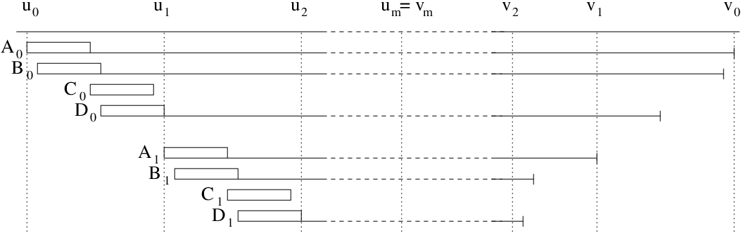
To illustrate this concept, consider the instances shown in Figure 2, where $p=4$. Up to time $9$ the two instances are indistinguishable. The overall optimal schedules are $(A,C,D,B)$ for the upper instance, and $(B,D,A)$ for the lower instance. So a left-to-right dynamic program must store the partial schedules $(B,D)$ and $(A,C)$ at time $9$.

We now amplify this construction by telescoping $n$ instances of this kind. As a result, we get an exponential number of partial schedules in some initial interval $[0,t_{0}]$ that are “indistinguishable” from each other by any left-to-right dynamic programming algorithm. Since the optimal solutions to those instances in $[0,t_{0}]$ are different, any such algorithm would have to keep track of exponentially many partial schedules.

For every $m$-bit string ${\bar{x}}=x_{0}x_{1}\ldots x_{m-1}$ we define an instance ${\cal J}_{\bar{x}}$ that consists of $4m$ jobs. The instance is partitioned into $m$ sub-instances, with sub-instance $i\in{\left\{0,\dots,m-1\right\}}$ containing jobs $A_{i}$, $B_{i}$, $C_{i}$, and $D_{i}$. We take $p$, the processing time, to be a sufficiently large integer (as explained later, any $p\geq 2m+3$ will work). For $i=0,\dots,m$, let

Let $t_{0}=u_{m}=v_{m}$. The time-scale is divided into intervals $[u_{i},u_{i+1}]$ for the left part and into intervals $[v_{i+1},v_{i}]$ for the second part. The release times and deadlines of the jobs are given in the following table.

For any given $m$-bit string ${\bar{x}}=x_{0}x_{1}\ldots x_{m-1}$, we define a schedule $R_{\bar{x}}$ of ${\cal J}_{\bar{x}}$ as follows for all $0\leq i\leq m-1$:

• •

  If $x_{i}=0$, $B_{i}$ and $D_{i}$ are scheduled at their release times and $A_{i}$ right before its deadline (that is, at time $v_{i+1}$.) $C_{i}$ is not scheduled.

• •

  If $x_{i}=1$, $A_{i}$ and $C_{i}$ are scheduled at their release times and $D_{i},B_{i}$ right before their deadlines (that is, at times $v_{i+1}$ and $v_{i+1}+p$, respectively.)

Proof: By routine inspection, $R_{\bar{x}}$ is a correct schedule. We claim that $R_{\bar{x}}$ is optimal. Let $\xi=\sum_{i}x_{i}$. Then schedule $R_{\bar{x}}$ contains $3m+\xi$ jobs. In this schedule each interval $[u_{i},u_{i+1}]$ has idle time $1$, and each interval $[v_{i+1},v_{i}]$ has idle time $x_{i}$. So the total idle time is $m+\xi\leq 2m$, and thus, for $p\geq 2m+3$, $R_{\bar{x}}$ is an optimal schedule.

It remains to show that every optimal schedule has the same job sequence as $R_{\bar{x}}$. For this purpose let $\bar{S}$ be an optimal schedule and let $S$ be a schedule obtained from $\bar{S}$ by left-shifting the jobs before $t_{0}$ and right-shifting the jobs after $t_{0}$. Formally every job scheduled before $t_{0}$ either starts at its release time or at the completion time of another job, and every job scheduled at $t_{0}$ or later completes either at its deadline or at a time where another job is started. Clearly the order in which the jobs appear in $\bar{S}$ and $S$ is the same.

By induction, we show for every $0\leq i\leq m-1$ that $S$ is identical with $R_{\bar{x}}$ in $[u_{i},u_{i-1}]\cup[v_{i+1},v_{i}]$. By induction hypothesis these intervals can contain no job from $A_{j},B_{j},C_{j},D_{j}$ for $j<i$. It shows that the only available jobs in $[u_{i},u_{i-1}]\cup[v_{i+1},v_{i}]$ are $A_{i},B_{i},C_{i},D_{i}$.

When $x_{i}=0$, the interval $[v_{i+1},v_{i}]$ must contain the job $A_{i}$, otherwise the idle time would be more than $p-2>2m$, which contradicts the optimality of $S$. Then the interval $[u_{i},u_{i+1}]$ cannot contain $C_{i}$, since this would imply that the period $[u_{i},u_{i}+p]$ is idle. Therefore this interval must contain the jobs $B_{i},D_{i}$, in that order.

When $x_{i}=1$, the intervals $[u_{i},u_{i+1}]$ and $[v_{i+1},v_{i}]$ must contain all four jobs, at least portions of it, otherwise the idle time would be at least $p>2m$. Job $C_{i}$ is tight. Therefore job $A_{i}$ must be scheduled at its release time. This in turn shows that $D_{i},B_{i}$ must be scheduled in the interval $[v_{i+1},v_{i}]$ in that order. $\Box$

A left-to-right dynamic algorithm is an algorithm ${\cal A}$ with the following properties:

• •

  It processes the jobs from left to right on the time axis, and for each time $t$ it constructs a collection ${\bf S}_{t}$ of partial schedules in the interval $[0,t]$. The schedules in ${\bf S}_{t}$ are obtained by extending schedules from ${\bf S}_{t^{\prime}}$, for $t^{\prime}<t$, by appending new jobs at the end. The final schedule is chosen from ${\bf S}_{t}$ for $t={d_{\mbox{\tiny max}}}$.

• •

  At each step $t$, ${\cal A}$ decides which non-expired jobs should be added to previous schedules. This decision is based on values of the release times and deadlines which are smaller or equal $t$ and on pairwise comparisons between deadlines that are greater than $t$.

Consider now the behavior of ${\cal A}$ on instances ${\cal J}_{\bar{x}}$. Until $t_{0}$, all these instances are indistinguishable to ${\cal A}$, since all jobs expired by time $t_{0}$ are identical, and the deadline ordering for the jobs. (For each $i$, the deadline ordering of $A_{i},B_{i},D_{i}$, does not depend on whether $x_{i}=0$ or $1$.) Thus at time $t_{0}$, for each ${\bar{x}}$, ${\cal A}$ would need to store a partial schedule that consist of the first $2m$ jobs from $R_{\bar{x}}$. So ${\cal A}$ would need to keep track of exponentially many partial schedules.

It should be noted that the maximization algorithm proposed by Carlier does fall into the framework described above. Although the algorithm, as shown, makes $n$ left-to-right passes along the time axis, each schedule $S^{k}_{t}$ depends only on schedules $S^{k^{\prime}}_{t^{\prime}}$ for $k^{\prime}\leq k$ and $t^{\prime}\leq t$. So the algorithm could be equivalently reformulated to compute all these schedules in just a single pass.

One may also ask what happens if some bounded look-ahead, say $\ell p$, is allowed in the algorithm. Our construction can be easily modified to show that this will also not work. To see this, simply add $\ell$ “tight” jobs to the instances, with release times $t_{0},t_{0}+p,\dots,t_{0}+(\ell-1)p$, and deadlines $t_{0}+p,\dots,t_{0}+\ell p$, respectively, and shift the right half of the instances by $\ell p$. The same result holds, if the algorithm is granted the ability to verify if the schedules in ${\bf S}_{t}$ are feasible or not. The details are left to the reader.

Our algorithm is based on a technique developed by Baptiste [1] for solving the weighted version of the problem. We show how to improve Baptiste’s $O(n^{7})$ time complexity exploiting the fact that the jobs have equal weights. Our algorithm can be thought of as a dual to the one in [1]. While Baptiste’s algorithm computes maximum weight schedules for a certain family of sub-instances, our algorithm considers similar sub-instances, but for given weights computes minimum makespans of schedules with given weights. In our case, the weight of a schedule is the number of jobs, and thus is bounded by $n$. This gives us a desired reduction in running time.

Proof: Our algorithm uses dynamic programming and it runs in $n$ phases. During the $k$-th phase we take under consideration only jobs $1,2,\ldots,k$. (Recall that jobs are ordered by their deadlines.) Let $\Theta^{\prime}={\left\{r_{i}+lp:\;i=1,\ldots,n;\;l=-1,0,\ldots,n\right\}}$. It is easy to see that $|\Theta^{\prime}|=O(n^{2})$. For each $\alpha\in\Theta^{\prime}$ and each $u\in{\left\{1\ldots k\right\}}$ we define:

${\cal J}^{k}_{\alpha}$ =  the set of all jobs $j\in{\left\{1,2,\dots,k\right\}}$ with $r_{j}\geq\alpha$.

$B^{k}_{\alpha,u}$ =  the minimal value $\beta\in\Theta^{\prime}$ such that it is possible to execute exactly $u$ jobs from ${\cal J}^{k}_{\alpha}$ in the interval $[\alpha+p,\beta]$.

If a schedule in the definition of $B^{k}_{\alpha,u}$ does not exist, we assume that $B^{k}_{\alpha,u}=+\infty$. It is convenient to extend this notation by setting $B^{k}_{\alpha,0}=\alpha+p$ for all $k\in{\left\{0,\ldots,n\right\}}$, $\alpha\in\Theta^{\prime}$, and $B^{k}_{\alpha,u}=+\infty$ for $k\in{\left\{0,\ldots,n\right\}}$, $\alpha\in\Theta^{\prime}$ and $u>k$.

Now we show how $B^{k}_{\alpha,u}$ depends on the values computed during the previous phase, i.e. $B^{k-1}_{\alpha^{\prime},u^{\prime}}$, for $\alpha^{\prime}\in\Theta^{\prime}$ and $u^{\prime}\in{\left\{0,\ldots,n\right\}}$. Let $k>0$, $\alpha$, $u>0$ be fixed, and let us consider a canonical schedule $S$ that satisfies the conditions defining $B^{k}_{\alpha,u}$:

(s1) exactly $u$ jobs from ${\cal J}^{k}_{\alpha}$ are executed in $S$,

(s2) all jobs are executed in the interval $[\alpha+p,\beta]$,

(s3) $\beta$ is minimal,

where $\beta=B^{k}_{\alpha,u}$. If $k\notin S$ then we have $B^{k}_{\alpha,u}=B^{k-1}_{\alpha,u}$. So from now on we will assume that $k\in S$, which implies $r_{k}\geq\alpha$. We will denote the number of jobs executed in $S$ before and after $k$ by $x$ and $y$, respectively. The starting time of job $k$ is denoted by $\gamma$. (See Fig 4.)

Since the jobs are ordered by their deadlines, and $S$ is canonical, we conclude that $S$ must satisfy the following conditions:

(s4) all the jobs executed after job $k$ are in ${\cal J}^{k-1}_{\gamma}$ and are executed in the interval $[\gamma+p,\beta]$,

(s5) all the jobs executed before job $k$ are in ${\cal J}^{k-1}_{\alpha}$ and are executed in the interval $[\alpha+p,\gamma]$,

(s6) $\gamma=\max(r_{k},B^{k-1}_{\alpha,x})$,

(s7) $\beta=B^{k-1}_{\gamma,y}$.

Notice that, if we knew the value of $x$, we could easily derive $\gamma$ using property (s6), and then derive $\beta$ using property (s7). As we do not know $x$, we have to iterate over all possible values $x=0,1,\ldots,u-1$, and choose the schedule with minimal $\beta$. Finally, we set $B^{k}_{\alpha,u}$ to $\min(B^{k-1}_{\alpha,u},\beta)$.

The algorithm is summarized in the pseudo-code below:

After the completion of the algorithm, the number of jobs executed in the optimal schedule is equal to the maximal value of $u$ such that $B^{n}_{-p,u}\neq+\infty$. (Recall that, by our convention, $\min(\Theta^{\prime})=-p$.) The optimal schedule itself can also be easily derived from the values stored in the array $B$ with the use of standard techniques.

The overall complexity of our algorithm is $O(n^{5})$, because each of $O(n^{4})$ values $B^{k}_{\alpha,u}$ is computed in linear time. $\Box$

References

- [1] P. Baptiste. Polynomial time algorithms for minimizing the weighted number of late jobs on a single machine with equal processing times. Journal of Scheduling, 2:245–252, 1999.
- [2] J. Carlier. Problèmes d’ordonnancement à durées égales. QUESTIO, 5(4):219–228, 1981.
- [3] M. Garey, D. Johnson, B. Simons, and R. Tarjan. Scheduling unit-time tasks with arbitrary release times and deadlines. SIAM Journal on Computing, 10(2):256–269, 1981.
- [4] B. Simons. A fast algorithm for single processor scheduling. In Proceedings IEEE 19th Annual Symposium on Foundations of Computer Science (FOCS’78), pages 246–252, 1978.