Maximum Mutual Information of Space-Time Block Codes
with Symbolwise Decodability

Maximum Mutual Information of Space-Time Block Codes with Symbolwise Decodability

1 Introduction

2 Preliminaries

3 Maximum Mutual Information (MMI) of SSDD and CLPOD

4 Numerical Result

5 Conclusion

References

2.1 Mathematical Model for MIMO System

2.2 Definitions of Codes

3.1 Equivalent Channel Model

3.2 MMI of SSDD

3.3 An expression of MMI of CLPOD

Abstract

In this paper, we analyze the performance of space-time block codes which enable symbolwise maximum likelihood decoding. We derive an upper bound of maximum mutual information (MMI) on space-time block codes that enable symbolwise maximum likelihood decoding for a frequency non-selective quasi-static fading channel. MMI is an upper bound on how much one can send information with vanishing error probability by using the target code.

An important problem in future telecommunication systems will be how to send large amount of data such as video through a wireless channel at high rate with high reliability in a mobile environment. One way to enable the high rate communication on the scattering-rich wireless channel is use of multiple transmit and receive antennas. It is well known that the capacity of a wireless channel linearly increases as the number of transmit and receive antennas under the condition that total power and bandwidth of signals are constant [1, 2]. A wireless communication system with multiple transmit and receive antennas is called multi-input multi-output (MIMO) system and an encoding/modulation method for MIMO system is called space-time code.

In the design of space-time codes, it is desirable to reduce the size of the circuit for encoding and decoding. Jiang et al. [7] and Khan et al. [8] derived a necessary and sufficient condition for symbolwise maximum likelihood (ML) decoding on linear dispersion codes (LDC) [6], and such code design is named single symbol decodable design (SSDD). Complex linear processing orthogonal design (CLPOD) [3], which is the subclass of SSDD, has full diversity and maximum coding gain because of an additional condition on codewords. Many researchers have studied concrete construction [4], rate [5], BER and the capacity utilization efficiency [6, 11] of CLPOD.

The capacity utilization efficiency of a code can be measured by calculating its attainable maximum mutual information (MMI). MMI of a code is defined as the capacity of a channel which consists of an encoder of the target code and the original channel, so it is an upper bound on how much one can send information with vanishing error probability by using the code. Therefore we know how much a space-time block code utilizes the capacity of wireless channel by calculating their MMI. MMI is also an important measure of an inner code of a concatenated code because it corresponds to maximum possible information rate with vanishing error probability by taking the block length of an outer code large. Hassibi and Hochwald [6] computed MMI of Alamouti’s code [9] and MMI of an example of rate-3/4 CLPOD and mentioned that these values are far below original channel capacity with more than one receive antenna. They also proposed LDCs whose MMI are close to original channel capacity for several numbers of transmit/receive antennas. Sandhu and Paulraj [11] derived the expression of MMI of general CLPOD and showed that for Rayleigh fading channel, the value equals to original channel capacity only when one receive antenna is used. However, there is no knowledge of MMI of SSDD, which is a subclass of LDC and includes CLPOD as a special case. The importance of this problem is also mentioned in the literature [7].

In this paper we compute MMI of SSDD over frequency non-selective quasi-static Rayleigh fading channel and clarify the necessary symbol rate at which SSDD utilizes full capacity of original channel. This paper is organized as follows: In Section 2, we introduce a mathematical model for MIMO systems and the definitions of SSDD and CLPOD. In Section 3, we derive an upper bound on MMI of SSDD. Also we give alternative derivation of the exact expression of MMI of CLPOD. In Section 4, we show the tightness of the upper bound on MMI of SSDD by comparing it with delay optimal complex orthogonal design (COD), which is a subclass of CLPOD at the same symbol rate. Then we clarify the necessary symbol rate of SSDD at which MMI of SSDD can attain original channel capacity. We show that the necessary symbol rate is much larger than that of CLPOD upper bounded by 3/4. Finally, Section 5 provides our conclusions.

Notation: Upper case letters denote matrices and bold lower case letter denote vectors; $\Re(\cdot)$ and $\Im(\cdot)$ denote real and imaginary part of complex number, respectively; $(\cdot)^{t}$ and $(\cdot)^{H}$ denote transpose and Hermitian transpose, respectively; $a_{ij}$ and $x_{i}$ denote the $(i,j)$ th entry of a matrix $A$ and $i$ th entry of a vector ${\bf x}$ , respectively; $I_{M}$ denotes the identity matrix of size $M$ ; $\det(\cdot)$ and $\mathop{\rm tr}\nolimits(\cdot)$ denote determinant and trace of a matrix, respectively; $\mathop{\rm diag}\nolimits({\bf x})$ is a diagonal matrix with ${\bf x}$ on its diagonal; $E_{A}[\cdot]$ and $E_{\bf x}[\cdot]$ denote expectation over random matrix $A$ and random vector ${\bf x}$ , respectively; covariance matrix of random vector ${\bf x}$ is denoted as $\Gamma_{\bf x}$ . We always index matrix and vector entries starting from 1. Complex and real field are denoted as ${\bf C}$ and ${\bf R}$ , respectively.

In this section, we introduce a mathematical model for MIMO system and define several space-time codes.

We consider a communication system that uses $M$ transmit antennas and $N$ receive antennas. Each transmit antenna simultaneously sends a narrow band signal through a frequency non-selective Rayleigh fading channel. The fading is assumed to be quasi-static so that the fading coefficients are constant for $T$ channel uses. We can write the relation between a transmitted block (or a codeword) $S$ and a received block $R$ as follows.

$\displaystyle R$	$\displaystyle=$	$\displaystyle\sqrt{\frac{\rho}{M}}SH+V$	(1)
$\displaystyle R$	$\displaystyle=$	$\displaystyle[r_{tm}]\in{\bf C}^{T\times N}$
$\displaystyle S$	$\displaystyle=$	$\displaystyle[s_{tm}]\in{\bf C}^{T\times M}$
$\displaystyle H$	$\displaystyle=$	$\displaystyle[h_{mn}]\in{\bf C}^{M\times N}$
$\displaystyle V$	$\displaystyle=$	$\displaystyle[v_{tm}]\in{\bf C}^{T\times N}$

$r_{tn}$	:	signal to $n$ th receive antenna at time $t$
$s_{tm}$	:	signal from $m$ th transmit antenna at time $t$
$h_{mn}$	:	fading coefficient between $m$ th transmit
		antenna and $n$ th receive antenna
$v_{tn}$	:	additive white Gaussian noise (AWGN) at
		$n$ th receive antenna at time $t$
$\rho$	:	SNR at each receive antenna

The fading coefficient $h_{mn}$ and AWGN $v_{n}$ are statistically independent complex Gaussian random variables with zero mean and unit variance. We assume that the receiver knows a realization of fading coefficients (i.e. receiver has perfect CSI (Channel State Information)) but the transmitter does not. The transmitted block is assumed to satisfy following power constraint:

\sum_{t=1}^{T}\sum_{m=1}^{M}|s_{tm}|^{2}=E\left[\mathop{\rm tr}\nolimits(SS^{*})\right]\leq TM.

(2)

Definition(LDC) [6]: A linear dispersion code (LDC) is a space-time code whose codeword $S$ is generated from information sequence ${\bf u}=[u_{1},\cdots,u_{2Q}]^{t}\in{\bf R}^{2Q}$ as

S=\sum_{q=1}^{2Q}u_{q}A_{q},

(3)

where $A_{q}\in{\bf C}^{T\times M}\ (q=1,\cdots,2Q)$ is called dispersion matrices.

Definition(SSDD) [7, 8]: A single symbol decodable design (SSDD) is an LDC whose dispersion matrices satisfy the following equations:

A_{q}^{H}A_{r}+A_{r}^{H}A_{q}=O_{M}\ (0\leq q\neq r\leq 2Q).

(4)

Jiang et al. [7] and Khan et al. [8] proved that a receiver can execute ML decoding for each symbol $u_{q}$ instead of each sequence ${\bf u}$ iff Eq. (4) holds. Applying Eq. (3) and Eq. (4) to Eq. (2), we have the following power constraint on ${\bf u}$ for SSDD:

\mathop{\rm tr}\nolimits(D_{A}\Gamma_{\bf u})\leq TM,\\

(5)

where $\Gamma_{\bf u}$ denotes the covariance matrix of the random vector ${\bf u}$ and

D_{A}=\mathop{\rm diag}\nolimits\left(\mathop{\rm tr}\nolimits(A_{1}^{H}A_{1}),\cdots,\mathop{\rm tr}\nolimits(A_{2Q}^{H}A_{2Q})\right).

(6)

Definition(CLPOD) [3]: A complex linear processing orthogonal design (CLPOD) is an SSDD whose dispersion matrices also satisfy the following equations:

A_{q}^{H}A_{q}=I_{M}\ (q=1,2,\cdots,2Q).

(7)

It is known that CLPOD achieves full diversity and maximum coding gain over all LDCs subject to a constant signal constellation and a constant number of dispersion matrices. For a code in the class of CLPOD, we may use following simple power constraint of on ${\bf u}$ :

\mathop{\rm tr}\nolimits(\Gamma_{\bf u})\leq T.

(8)

Definition(COD) [3]: A complex orthogonal design (COD) is an CLPOD whose dispersion matrices satisfy following constraint:

•

$A_{q}\in\{0,\pm 1,\pm j\}^{T\times M}\ (1\leq q\leq 2Q)$
•

If $A_{2q-1}$ or $A_{2q}\ (1\leq q\leq Q)$ has a nonzero $(i,j)$ entry, then $(i,j)$ entries of $A_{2r-1}$ and $A_{2r}\ (1\leq r\neq q\leq Q)$ are all zero.

In this section, we discuss capacity utilization of space-time codes with symbolwise decodability by deriving their MMI. MMI of CLPOD is derived in [11], but MMI of SSDD is unknown because the key equation Eq. (3) in [11] does not hold for general SSDD. We give an upper bound on MMI of SSDD and alternative derivation of exact MMI of CLPOD.

We want to calculate mutual information between input ${\bf u}$ of SSDD or CLPOD encoder and output $R$ of MIMO channel, but in Eq. (1), ${\bf u}$ is hidden in $S$ . So we start with extracting a relation between ${\bf u}$ and $R$ from Eq. (1). The same derivation of the equivalent channel can be found in [6].

We define new vectors and new matrices as follows:

	$\displaystyle{\bf r}$	$\displaystyle=[{\bf r}_{R,1}^{t},{\bf r}_{I,1}^{t},\cdots,{\bf r}_{R,N}^{t},{\bf r}_{I,N}^{t}]^{t}\in{\bf R}^{2TN},$
	$\displaystyle{\bf w}$	$\displaystyle=[{\bf v}_{R,1}^{t},{\bf v}_{I,1}^{t},\cdots,{\bf v}_{R,N}^{t},{\bf v}_{I,N}^{t}]^{t}\in{\bf R}^{2TN},$
	$\displaystyle{\bf g}_{n}$	$\displaystyle=[{\bf h}_{R,n}^{t},{\bf h}_{I,n}^{t}]^{t},$
	$\displaystyle B_{q}$	$\displaystyle=\left[\begin{array}[]{@{\,}cc@{\,}}A_{R,q}&-A_{I,q}\\ A_{I,q}&A_{R,q}\\ \end{array}\right],$
	$\displaystyle G$	$\displaystyle=\left[\begin{array}[]{@{\,}ccc@{\,}}B_{1}{\bf g}_{1}&\ldots&B_{2Q}{\bf g}_{1}\\ \vdots&\ddots&\vdots\\ B_{1}{\bf g}_{N}&\ldots&B_{2Q}{\bf g}_{N}\\ \end{array}\right]\in{\bf R}^{2NT\times 2Q},$

where the vectors ${\bf x}_{R,n},\ {\bf x}_{I,n}$ denote the $n$ th column of real and imaginary part of the matrix $X$ respectively. Then Eq. (1) can be equivalently written as

{\bf r}=\sqrt{\frac{\rho}{M}}G{\bf u}+{\bf w}.

(9)

The equivalent channel matrix $G$ is known to the receiver because the original channel matrix $H$ and the dispersion matrices $\{A_{q}\}$ are known to receiver. Note also that the vector ${\bf r}$ is equivalent to received block $R$ . Therefore MMI of SSDD with $M$ transmit antennas, $N$ receive antennas, $T$ block length, $Q$ complex information symbols (i.e., $2Q$ real information symbols) and dispersion matrices $\{A_{q}\}$ at SNR $\rho$ is equal to

	$\displaystyle C_{\rm SSDD}(\rho,M,N,T,Q,\{A_{q}\})$						(10)
		$\displaystyle=$	$\displaystyle\frac{1}{T}\max_{p({\bf u}:\mathop{\rm tr}\nolimits(D_{A}\Gamma_{\bf u})\leq TM)}I({\bf u};{\bf r},G),$				(10)

where the factor $1/T$ normalizes the mutual information for the $T$ channel uses spanned by SSDD and $\mathop{\rm tr}\nolimits(D_{A}\Gamma_{\bf u})\leq TM$ denotes power constraint on ${\bf u}$ . By the derivation similar to [1, 6], we can rewrite Eq. (10) as

		$\displaystyle C_{\rm SSDD}(\rho,M,N,T,Q,\{A_{q}\})=$
		$\displaystyle\frac{1}{2T}\max_{\Gamma_{\bf u}:\mathop{\rm tr}\nolimits(D_{A}\Gamma_{\bf u})\leq TM}E_{H}\left[\log\det\left(I_{2Q}+\frac{2\rho}{M}G^{t}G\Gamma_{\bf u}\right)\right],$		(11)

where the expectation is taken over the distribution of the original channel matrix $H$ . It is difficult to simplify Eq. (11), but we can derive its upper bound by recognizing that $\log\det(\cdot)$ is concave function over the set of positive semi-definite matrices and using Jensen’s inequality. We explain detailed derivation of upper bound as follows.

Since the covariance matrix $\Gamma_{\bf u}$ is positive semi-definite, there is at least one square matrix $F=\sqrt{\Gamma_{\bf u}}$ that satisfies $FF^{t}=\Gamma_{\bf u}$ . So using determinant identity $\det(I_{m}+AB)=\det(I_{n}+BA),\ A\in{\bf R}^{m\times n},\ B\in{\bf R}^{n\times m}$ , we rewrite Eq. (11) as

	$\displaystyle C_{\rm SSDD}$	$\displaystyle=$	$\displaystyle\frac{1}{2T}\max_{\Gamma_{\bf u}:\mathop{\rm tr}\nolimits(D_{A}{\tilde{\Gamma}_{\bf u}})\leq TM}$
			$\displaystyle E_{H}\left[\log\det\left(I_{2Q}+\frac{2\rho}{M}F^{t}G^{t}GF\right)\right].$

The term $\log\det(I_{2Q}+(2\rho/M)F^{t}G^{t}GF)$ in Eq. () is a concave function of $G^{t}G$ because for any positive semi-definite matrices $A,\ B\in R^{2Q\times 2Q}$ and for any real number $0\leq\lambda\leq 1$ , the inequality

$\displaystyle\log\det\left(I_{2Q}+\frac{2\rho}{M}F^{t}\left\{\lambda A+(1-\lambda)B\right\}F\right)$
	$\displaystyle\geq$	$\displaystyle\lambda\log\det\left(I_{2Q}+\frac{2\rho}{M}F^{t}AF\right)$
		$\displaystyle+(1-\lambda)\log\det\left(I_{2Q}+\frac{2\rho}{M}F^{t}BF\right)$

holds. Therefore we may apply Jensen’s inequality to Eq. () to obtain an upper bound of MMI of SSDD

	$\displaystyle C_{\rm SSDD}$	$\displaystyle\leq$	$\displaystyle\frac{1}{2T}\max_{\Gamma_{\bf u}:\mathop{\rm tr}\nolimits(D_{A}{\tilde{\Gamma}_{\bf u}})\leq TM}$
			$\displaystyle\log\det\left(I_{2Q}+\frac{2\rho}{M}F^{t}E_{H}[G^{t}G]F\right).$

The matrix $G^{t}G$ in Eq. () is a function of the set of dispersion matrices $\{A_{q}\}$ as well as the channel matrix $H$ . We can simplify $G^{t}G$ by using a necessary and sufficient condition Eq. (4) for SSDD. From definitions, we have

G^{t}G=\sum_{n=1}^{N}\left[\begin{array}[]{@{\,}ccc@{\,}}{\bf g}_{n}^{t}B_{1}^{t}B_{1}{\bf g}_{n}&\ldots&{\bf g}_{n}^{t}B_{1}^{t}B_{2Q}{\bf g}_{n}\\ \vdots&\ddots&\vdots\\ {\bf g}_{n}^{t}B_{2Q}^{t}B_{1}{\bf g}_{n}&\ldots&{\bf g}_{n}^{t}B_{2Q}^{t}B_{2Q}{\bf g}_{n}\\ \end{array}\right]

(14)

and

$\displaystyle{\bf g}_{n}^{t}B_{q}^{t}B_{r}{\bf g}_{n}$			(15)
	$\displaystyle=$	$\displaystyle{\bf h}_{R,n}^{t}\Re\left(A_{q}^{H}A_{r}\right){\bf h}_{R,n}+{\bf h}_{I,n}^{t}\Re\left(A_{q}^{H}A_{r}\right){\bf h}_{I,n}$
		$\displaystyle-{\bf h}_{R,n}^{t}\left\{\Im\left(A_{q}^{H}A_{r}\right)-\Im\left(A_{q}^{H}A_{r}\right)^{t}\right\}{\bf h}_{I,n}.$

To simplify Eq. (15), we use the following lemma.

Lemma:If the set $\{A_{q}\}$ of $2Q$ matrices satisfying Eq. (4) then following equalities hold for any real vectors ${\bf x},\ {\bf y}\in{\bf R}^{M}$ :

{\bf x}^{t}\Re(A_{q}^{H}A_{r}){\bf x}=0,\ 1\leq q\neq r\leq 2Q,

{\bf x}^{t}\left\{\Im\left(A_{q}^{H}A_{r}\right)-\Im\left(A_{q}^{H}A_{r}\right)^{t}\right\}{\bf y}=0,\ 1\leq q,r\leq 2Q.

Proof:

$\displaystyle{\bf x}^{t}\Re(A_{q}^{H}A_{r}){\bf x}$	$\displaystyle=$	$\displaystyle\frac{1}{2}\left\{{\bf x}^{t}\Re(A_{q}^{H}A_{r}){\bf x}+{\bf x}^{t}\Re(A_{q}^{H}A_{r}){\bf x}\right\}$
	$\displaystyle=$	$\displaystyle\frac{1}{2}{\bf x}^{t}\Re(A_{q}^{H}A_{r}+A_{r}^{H}A_{q}){\bf x}$
	$\displaystyle=$	$\displaystyle 0$

Q.E.D.
By using Lemma, we obtain

$\displaystyle G^{t}G=\sum_{n=1}^{N}\mathop{\rm diag}\nolimits\left[\right.$	$\displaystyle{\bf h}_{R,n}^{t}\Re\left(A_{1}^{H}A_{1}\right){\bf h}_{R,n}$
	$\displaystyle+{\bf h}_{I,n}^{t}\Re\left(A_{1}^{H}A_{1}\right){\bf h}_{I,n},$
	$\displaystyle\cdots,$
	$\displaystyle{\bf h}_{R,n}^{t}\Re\left(A_{2Q}^{H}A_{2Q}\right){\bf h}_{R,n}$
	$\displaystyle\left.+{\bf h}_{I,n}^{t}\Re\left(A_{2Q}^{H}A_{2Q}\right){\bf h}_{I,n}\right].$	(16)

Denoting $m$ th entries of ${\bf h}_{R,n}$ and ${\bf h}_{I,n}$ and $(l,m)$ entry of $\Re(A_{q}^{t}A_{q})$ as $h_{R,n}(m),\ h_{I,n}(m)$ and $a_{q}(l,m)$ , respectively, we have

$\displaystyle E_{H}\left[{\bf h}_{R,n}^{t}\Re(A_{q}^{t}A_{q}){\bf h}_{R,n}+{\bf h}_{I,n}\Re(A_{q}^{r}A_{q}){\bf h}_{I,n}\right]$			(17)
	$\displaystyle=$	$\displaystyle\sum_{m=1}^{M}a_{q}(m,m)E\left[h_{R,n}(m)^{2}\right]$
		$\displaystyle+\sum_{l<m}^{M}a_{q}(l,m)E\left[h_{R,n}(l)\right]E\left[h_{R,n}(m)\right]$
		$\displaystyle+\sum_{m=1}^{M}a_{q}(m,m)E\left[h_{I,n}(m)^{2}\right]$
		$\displaystyle+\sum_{l<m}^{M}a_{q}(l,m)E\left[h_{I,n}(l)\right]E\left[h_{I,n}(m)\right]$
	$\displaystyle=$	$\displaystyle\frac{1}{2}\sum_{m=1}^{M}a_{q}(m,m)+\frac{1}{2}\sum_{m=1}^{M}a_{q}(m,m)$	(18)
	$\displaystyle=$	$\displaystyle\mathop{\rm tr}\nolimits\left[\Re(A_{q}^{t}A_{q})\right]$
	$\displaystyle=$	$\displaystyle\mathop{\rm tr}\nolimits(A_{q}^{H}A_{q}),$

where Eq. (17) follows from the statistical independence among channel gains and Eq. (18) follows from that the mean and variance of channel gains $h_{R,n}(m),\ h_{I,n}(m)$ are 0 and 1/2, respectively. Therefore we have

E_{H}\left[G(H)^{t}G(H)\right]=D_{A}.

(19)

Substituting Eq. (19) into Eq. (), we obtain

C_{\rm SSDD}\leq\frac{1}{2T}\max_{\Gamma_{\bf u}:\mathop{\rm tr}\nolimits(D_{A}{\tilde{\Gamma}_{\bf u}})\leq TM}\log\det\left(I_{2Q}+\frac{2\rho N}{M}D_{A}{\tilde{\Gamma}}_{\bf u}\right).

(20)

We simply choose $(TM/2Q)I_{2Q}$ as $D_{A}\Gamma_{\bf u}$ to maximize the term $\log\det(\cdot)$ in Eq. (20) and get

C_{\rm SSDD}\leq\frac{Q}{T}\log\left(1+\rho N\cdot\frac{T}{Q}\right).

(21)

The maximum symbol rate $Q/T$ of SSDD for $M$ is unknown unlike CLPOD [5] or COD [5, 4]. In section 4, we numerically evaluate Eq. (21) and show necessary rate of SSDD at which MMI of SSDD can utilize full channel capacity. In Section 4, we search the tightness of the upper bound Eq.(21) by comparing it with delay optimal COD at the same symbol rate.

Unlike SSDD, we can derive an exact expression of MMI of CLPOD due to the additional condition Eq. (7). Sandhu and Paulraj [11] derived an expression MMI of CLPOD. We give alternative derivation of MMI of CLPOD by using the result of MMI of SSDD in previous subsection. We also show that MMI of CLPOD relates the capacity of another channel whose parameter setting (i.e., number of transmit/receive antennas and SNR at each receive antenna) differs from original one. In [11], MMI for given channel realization $H$ is computed but we compute average MMI over $H$ .

Denoting MMI of CLPOD as $C_{\rm CLPOD}$ , we have

$\displaystyle C_{\rm CLPOD}$			(22)
	$\displaystyle=$	$\displaystyle\frac{1}{2T}\max_{\Gamma_{\bf u}:\mathop{\rm tr}\nolimits(\Gamma_{\bf u})\leq M}$
		$\displaystyle E_{H}\left[\log\det\left(I_{2Q}+\frac{2\rho}{M}G^{t}G\Gamma_{\bf u}\right)\right]$
	$\displaystyle=$	$\displaystyle\frac{1}{2T}\max_{\Gamma_{\bf u}:\mathop{\rm tr}\nolimits(\Gamma_{\bf u})\leq M}$
		$\displaystyle E_{H}\left[\log\det\left(I_{2Q}+\frac{2\rho}{M}\sum_{m=1}^{M}\sum_{n=1}^{N}\|h_{mn}^{2}\|\Gamma_{\bf u}\right)\right]$
	$\displaystyle=$	$\displaystyle\frac{1}{2T}E_{H}\Bigg[\log\det\Bigg(I_{2Q}$
		$\displaystyle+\frac{2\rho}{M}\sum_{m=1}^{M}\sum_{n=1}^{N}\|h_{mn}^{2}\|\cdot\frac{M}{2Q}I_{2Q}\Bigg)\Bigg]$
	$\displaystyle=$	$\displaystyle\frac{Q}{T}E_{H}\left[\log\left(1+\frac{\rho}{Q}\sum_{m=1}^{M}\sum_{n=1}^{N}\|h_{mn}\|^{2}\right)\right]$

where the first equality Eq. (22) follows from Eq. (11) and the second equality Eq. () follows from using additional condition Eq. (7) of CLPOD in Eq. (16). Note that MMI of CLPOD does not depend on the choice of the set of dispersion matrices $\{A_{q}\}$ . On the other hand, the capacity of MIMO fading channel with $MN$ transmit antennas and 1 receive antenna at SNR $MN\rho/Q$ equals to

E\left[\log\left(1+\frac{\rho}{Q}\sum_{i=1}^{MN}|h_{i}|^{2}\right)\right],

(24)

where $h_{i}\ (i=1,\cdots,MN)$ are statistically independent complex Gaussian random variable with zero mean and unit variance [1, 2]. Therefore denoting channel capacity with $M^{\prime}$ transmit antennas and $N^{\prime}$ receive antennas at SNR $\rho^{\prime}$ as $C(\rho^{\prime},M^{\prime},N^{\prime})$ , we have a relation of MMI of CLPOD and channel capacity

C_{\rm CLPOD}(\rho,M,N,T,Q)=\frac{Q}{T}C\left(\frac{MN}{Q}\rho,MN,1\right).

(25)

From Eq. (25), we have three important observations.

•

It is well known that, at high SNR, the channel capacity is mainly dominated by the value of $\min\{M,N\}\log\rho$ [1, 2]. On the other hand, the third argument of the right hand of Eq. (25) is 1, which corresponds to the number of receive antennas. Therefore increasing numbers of both transmit and receive antennas does not increase MMI of CLPOD.
•

$C_{\rm CLPOD}$ is proportional to symbol rate $Q/T$ . However it is known that for more than three transmit antennas, maximum symbol rate achieved by CLPOD is equal to or less than 3/4 [5].
•

Under the condition that the symbol rate is constant, the delay optimal code i.e., the code having the minimum block length $T$ and the minimum number $Q$ of complex symbols has largest MMI.

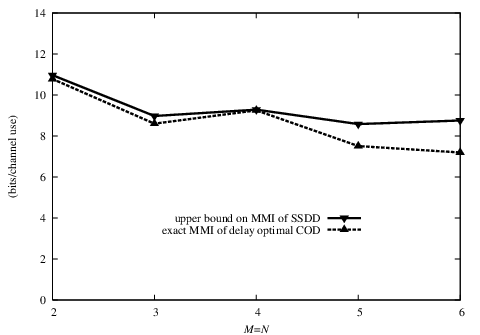
To show the tightness of Eq. (21), the upper bound of MMI of SSDD and exact MMI of delay optimal COD are shown in Fig. 1. We set SNR $\rho$ at 30[dB] and use parameters in Table 1 for computation, where design parameters $Q,\ T$ for COD is delay optimal one [4] and the symbol rate of SSDD is same as that of COD. Fig. 1 shows that under the same rate condition, the upper bound of MMI of SSDD is close to the exact MMI of COD for 2 to 4 transmit/receive antennas especially. Therefore we may regard Eq. (21) as a tight upper bound on MMI of SSDD.

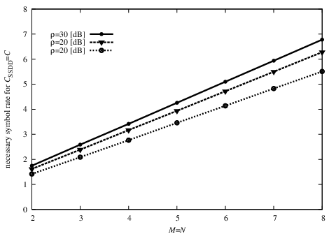
We give the necessary symbol rate of SSDD at which MMI of SSDD can achieve channel capacity at $\rho=$ 10, 20 and 30[dB] for 2 to 8 transmit/receive antennas, in Figure 2. We see that this value linearly increases as $M$ and this value is needed to be much larger than that of CLPOD upper bounded by 3/4.

	SSDD	COD
$M=N$	$Q/T$	$Q$	$T$	$Q/T$
2	1	2	2	1
3	3/4	3	4	3/4
4	3/4	3	4	3/4
5	2/3	10	15	2/3
6	2/3	20	30	2/3

Table 1: Parameter setting of SSDD and COD for 2 to 6 antennas

Refer to caption — Figure 1: Comparison between the upper bound of MMI of SSDD and exact MMI of delay optimal COD for 2 to 6 antennas at $\rho=30$ [dB]

In this paper we gave a tight upper bound of MMI of SSDD and alternative derivation of an exact expression of MMI of CLPOD. We showed the necessary symbol rate of SSDD at which MMI of SSDD can attain channel capacity and these value are much larger than the symbol rate of CLPOD. To find out more about performance of SSDD, the research of the maximum symbol rate of SSDD is needed.

[1] E. Telatar, “Capacity of multi-antenna Gaussian channels,” Europ. Trans. Telecommun, vol.10, pp.585-595, Nov. 1999.
[2] G. J. Foschini, “Layered space-time architecture for wireless communication in a fading environment when using multi-element antennas,” Bell Labs Tech. J., vol.1, pp 41-59, Autumn 1996.
[3] V. Tarokh, H. Jafarkhani and A. R. Calderbank, “Space-time block codes from orthogonal designs,” IEEE Trans. Inform. Theory, vol.45, pp.1456-1467, July. 1999.
[4] X. B. Liang, “Orthogonal designs with maximal rates,” IEEE Trans. Inform. Theory, vol.49, pp.2468-2503, Oct. 2003.
[5] H. W. Wang and X. G. Xia, “Upper bound of rates of complex orthogonal space-time block codes,” IEEE Trans. Inform. Theory, vol.49, pp.2788-2796, Oct. 2003.
[6] B. Hassibi and B. M. Hochwald, “High-rate codes that are linear in space and time,” IEEE Trans. Inform. Theory, vol.48, pp.1804-1824, July. 2002.
[7] Y. Jiang, R. Koetter and A. C. Singer, “On the separability of demodulation and decoding for communications over multi-antenna block-fading channels,” IEEE Trans. Inform. Theory, vol.49, pp.2709-2713, Oct. 2003.
[8] M. Z. A. Khan, B. S. Rajan and M. H. Lee, “On single-symbol and double-symbol decodable STBCs,” Proc. of ISIT 2003, June 30-July 5, Yokohama, Japan.
[9] S. M. Alamouti, “A simple transmit diversity technique for wireless communications,” IEEE J. Select. Areas Commun., vol.16, pp.1451-1458, Oct. 1998.
[10] T. M. Cover and J. A. Thomas, “Elements of information theory,” Wiley Interscience, 1991.
[11] S. Sandhu and A. Paulraj, “Space-time block codes: A capacity perspective,” IEEE Commun. Lett., vol.4, pp.384-386, Dec. 2000.

$\displaystyle{\bf x}^{t}\left\{\Im\left(A_{q}^{H}A_{r}\right)-\Im\left(A_{q}^{H}A_{r}\right)^{t}\right\}{\bf y}$

$\displaystyle=$

$\displaystyle{\bf x}^{t}\left\{\Im\left(A_{q}^{H}A_{r}\right)+\Im\left(A_{r}^{H}A_{q}\right)\right\}{\bf y}$

$\displaystyle=$

$\displaystyle{\bf x}^{t}\left\{\Im\left(A_{q}^{H}A_{r}+A_{r}^{H}A_{q}\right)\right\}{\bf y}$

$\displaystyle=$

$\displaystyle 0$