in Proceedings of the ECAI Workshop on Spatial and
Temporal Reasoning, pp. 135-139, Valencia, Spain, 2004:
A TCSP-like decidable
constraint language generalising existing cardinal
direction relationsThanks: TCSPs stands for Temporal Constraint
Satisfaction Problems, a well-known constraint-based
temporal framework [6].
Abstract
We define a quantitative constraint language subsuming two calculi well-known in QSR33 3 Qualitative Spatial Reasoning.: Frank’s cone-shaped and projection-based calculi of cardinal direction relations. The language is based on convex constraints of the form , with and : the meaning of such a constraint is that point belongs to the (convex) cone-shaped area rooted at , and bounded by angles and . The general form of a constraint is a disjunction of the form , with , , being a convex constraint as described above: the meaning of such a general constraint is that, for some , holds. A conjunction of such general constraints is a TCSP-like CSP, which we will refer to as an SCSP (Spatial Constraint Satisfaction Problem). We describe how to compute converse, intersection and composition of SCSP constraints, allowing thus to achieve path consistency for an SCSP. We show how to translate a convex constraint into a conjunction of linear inequalities on variables consisting of the arguments’ coordinates. Our approach to effectively solving a general SCSP is then to adopt a solution search algorithm using (1) path consistency as the filtering method during the search, and (2) the Simplex algorithm, guaranteeing completeness, at the leaves of the search tree.
Keywords: Constraint Satisfaction, Spatial reasoning, Geometric Reasoning, Knowledge Representation, Qualitative Reasoning, Quantitative Reasoning
WORK EXACTLY AS REJECTED AT THE MAIN ECAI11 1 European Conference on Artificial Intelligence. 200422 2 The reviews are added to the actual paper, after the references, for potential people interested in objectivity of conferences’ reviewing processes.
1 Introduction
Conciliating qualitative reasoning and quantitative reasoning in KR&R systems:
a way to systems
representationally more flexible,
cognitively more plausible,
and, computationally, with the advantage of having the choice between
a purely-quantitative and a
qualitative-computations-first behaviours.
Knowledge representation (KR) systems allowing for the representation of both qualitative knowledge and quantitative knowledge are more than needed by modern applications (see, e.g., [2]), which, depending on the level of detail of the knowledge to be represented, may feel happy with a high-level, qualitative language, or need to use a low-level, quantitative language. Qualitative languages suffer from what Forbus et al. [7] refer to as the poverty conjecture, but have the advantage of behaving computationally better. On the other hand, quantitative languages do not suffer from the poverty conjecture, but have a slow computatinal behaviour. Thus, such a KR system will feel happier when the knowledge at hand can be represented in a purely qualitative way, for it can then get rid of heavy numeric calculations, and restrict its computations to a manipulation of symbols, consisting, in the case of constraint-based languages in the style of the Region-Connection Calculus RCC-8 [15], mainly in computing a closure under a composition table.
An important question raised by the above discussion is clearly how to augment the chances of a qualitative/quantitative KR system to remain at the qualitative level. Consider, for instance, QSR constraint-based, RCC-8-like languages. Given the poverty conjecture, which corresponds to the fact that such a language can make only a finite number of distinctions, reflected by the number of its atomic relations, one way of answering the question could be to integrate more than one QSR language within the same KR system. The knowledge at hand is then handled in a quantitative way only in the extreme case when it can be represented by none of the QSR languages which the system integrates.
One way for a KR system, such as described above, to reason about its knowledge is to start with reasoning about the qualitative part of the knowledge, which decomposes, say, into n components, one for each of the QSR languages the system integrates. For RCC-8-like languages, this can be done using a constraint propagation algorithm such as the one in [1]. If in either of the n components, an inconsistency has been detected, then the whole knowledge has been detected to be inconsistent without the need of going into low-level details. If no inconsistency has been detected at the high, qualitative level, then the whole knowledge needs translation into the unifying quantitative language, and be processed in a purely quantitative way. But even when the high-level, qualitative computations fail to detect any inconsistency, they still potentially help the task of the low-level, purely quantitative computations. The situation can be compared to standard search algorithms in CSPs, where a local-consistency preprocessing is applied to the whole knowledge to potentially reduce the search space, and eventually detect the knowledge inconsistency, before the actual search for a solution starts.
With the above considerations in mind, we consider the integration of Frank’s cone-shaped and projection-based calculi of cardinal direction relations [8], well-known in QSR. A complete decision procedure for the projection-based calculus is known from Ligozat’s work [12]. For the other calculus, based on a uniform 8-sector partition of the plane, making it more flexible and cognitively more plausible, no such procedure is known. For each of the two calculi, the region of the plane associated with each of the atomic relations is convex, and given by the intersection of two half-planes. As a consequence, each such relation can be equivalently written as a conjunction of linear inequalities on variables consisting of the coordinates of the relation’s arguments. We consider a more general, qualitative/quantitative language, which, at the basic level, expresses convex constraints of the form , where is a cone-shaped or projection-based atomic relation of cardinal directions, or of the form , with and : the meaning of , in particular, is that point belongs to the (convex) cone-shaped area rooted at , and bounded by angles and . We refer to such constraints as basic constraints: qualitative basic constraint in the former case, and quantitative basic constraint in the latter. A conjunction of basic constraints can be solved by first applying constraint propagation, based on a composition operation to be defined, which is basically the spatial counterpart of composition of two TCSP constraints [6]. If the propagation detects no inconsisteny then the knowledge is translated into a system of linear inequalities, and solved with the well-known Simplex algorithm. The preprocessing of the qualitative component of the knowledge can be done with a constraint propagation algorithm such as the one in [1], and needs the composition tables of the cardinal direction calculi, which can be found in [8].
The general form of a constraint is , which we also represent as , where , for all , is a basic constraint, either qualitative or quantitative. The meaning of such a general constraint is that, either of the basic constraints is satisfied, i.e., . A general constraint is qualitative if it is the disjunction of qualitative basic constraints of one type, cone-shaped or projection-based; it is quantitative otherwise. The language can be looked at as the spatial counterpart of Dechter et al.’s TCSPs [6]: the domain of a TCSP variable is , symbolising continuous time, whereas the domain of an SCSP variable is the cross product , symbolising the continuous 2-dimensional space.
Due to space limitations, we restrict the presentation to the unifying TCSP-like constraint language, will all the tools required to convince the reader that the work is the description of an implementable KR&R system, consisting in a search algorithm using path consistency as the filtering procedure during the search, and the Simplex algorithm as a completeness guarantee, at the leaves of the search space.
2 Constraint satisfaction problems
A constraint satisfaction problem (CSP) of order consists of:
- 1.
a finite set of variables, ;
- 2.
a set (called the universe of the problem); and
- 3.
a set of constraints on values from which may be assigned to the variables.
An -ary constraint is of the form , and asserts that the values assigned to the variables , respectively, are so that the -tuple belongs to the -ary relation (an -ary relation over the universe is any subset of ). An -ary CSP is one of which the constraints are -ary constraints. We will be concerned exclusively with binary CSPs.
For any two binary relations and , is the intersection of and , is the union of and , is the composition of and , and is the converse of ; these are defined as follows:
Three special binary relations over a universe are the empty relation which contains no pairs at all, the identity relation , and the universal relation .
2.1 Constraint matrices
A binary constraint matrix of order over is an -matrix, say , of binary relations over verifying the following:
A binary CSP of order over a universe can be associated with the following binary constraint matrix, denoted :
- 1.
Initialise all entries to the universal relation:
- 2.
Initialise the diagonal elements to the identity relation:
- 3.
For all pairs of variables on which a constraint is specified: .
2.2 Strong -consistency, refinement
Let be a CSP of order , its set of variables and its universe. An instantiation of is any -tuple of , representing an assignment of a value to each variable. A consistent instantiation is an instantiation which is a solution: . is consistent if it has at least one solution; it is inconsistent otherwise. The consistency problem of is the problem of verifying whether is consistent.
Let be a subset of . The sub-CSP of generated by , denoted , is the CSP with as the set of variables, and whose constraint matrix is obtained by projecting the constraint matrix of onto : . is -consistent [9, 10] (see also [4]) if for any subset of containing variables, and for any variable , every solution to can be extended to a solution to . is strongly -consistent if it is -consistent, for all .
-consistency, -consistency and -consistency correspond to node-consistency, arc-consistency and path-consistency, respectively [13, 14]. Strong -consistency of corresponds to what is called global consistency in [5]. Global consistency facilitates the important task of searching for a solution, which can be done, when the property is met, without backtracking [10].
A refinement of is a CSP with the same set of variables, and such that: .
3 A spatial counterpart of TCSPs: Spatial Constraint Satisfaction Problems (SCSPs)
TCSPs (Temporal Constraint Satisfaction Problems) is a constraint-based framewrok well-known in Temporal Reasoning [6]. We provide a spatial counterpart of TCSPs, which we refer to as SCSPs —Spatial Constraint Satisfaction Problems. The domain of an SCSP variable is the cross product , which we look at as the set of points of the 2-dimensional space. As for a TCSP, an SCSP will have unary constraints and binary constraints, and unary constraints can be interpreted as special binary constraints by choosing an origin of the 2-dimensional space —space .
We first define some more terminology to be used in the rest of the paper. We make use of a Cartesian system of coordinates . The -axis is the origin of angles, and the anticlockwise orientation is the positive orientation for angles. Given that we use the set as the universe of angles (measured in radians), if two angles and are so that , the interval will represent the union . Given a positive real number and a strictly positive integer , we denote by the remainder of the integral division of by . Furthermore, given any , the difference will measure the anticlockwise (angular) distance of relative to : i.e., ; similarly, the sum of and is defined as .
Definition 1 (SCSP).
An SCSP consists of (1) a finite number of variables ranging over the universe of points of the 2-dimensional space (henceforth 2D-points); and (2) SCSP constraints on the variables.
An SCSP constraint is either unary or binary, and either basic or disjunctive. A basic constraint is (1) of the form , being equality, or (2) of the general form (binary) or (unary), with , , . ‘’ and ‘’ stand, respectively, for the left open bracket ‘(’ and the left close bracket ‘[’. Similarly, ‘’ and ‘’ stand, respectively, for the right open bracket ‘)’ and the right close bracket ‘]’. A graphical illustration of a general basic constraint is provided in Figure 1.
A disjunctive constraint is of the form (binary) or (unary), with and , , being basic constraints as described above: in the binary case, the meaning of such a disjunctive constraint is that, for some , holds; similarly, in the unary case, the meaning is that, for some , holds. A unary constraint may be seen as a special binary constraint if we consider an origin of the World (space ), represented, say, by a variable : is then equivalent to . Unless explicitly stated otherwise, we assume, in the rest of the paper, that the constraints of an SCSP are all binary.
An SCSP constraint is convex if, given an instantiation of , the set of points satisfying is a convex subset of the plane. A universal SCSP constraint is an SCSP constraint of the form : the knowledge consisting of such a constraint is equivalent to “no knowledge”, i.e., any instantiation of the pair satisfies it. A universal constraint is also a convex constraint. A convex SCSP is an SCSP of which all the constraints are convex. Given its similarity with an STP (Simple Temporal Problem) [6], we refer to a convex SCSP as an SSP (Simple Spatial Problem). An SCSP is basic if all its constraints are basic. We refer to a basic SCSP as a BSP (Basic Spatial Problem). Note that a BSP may have pairs of variables on which no constraint is specified (the implicit constraint on such pairs is then the universal relation , which we also refer to as ).
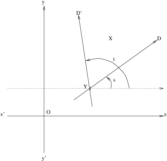
The standard path consistency procedure for binary CSPs is guided by three algebraic operations, the converse of a constraint, the composition of two constraints, and the intersection of two constraints. These are defined below for SCSP basic constraints. The case of general (possibly disjunctive) constraints is obtainable from the case of basic constraints.
3.1 The converse of an SCSP basic constraint
The converse of an SCSP relation is the SCSP relation such that, for all , , iff . We refer to the constraint as the converse of the constraint . The converse of is clearly . The converse of an SCSP basic constraint is the SCSP basic constraint , which can be explained by the simple fact that, given any instantiation of the pair satisfying the constraint , the angle formed by the directed line with the -axis is obtained by adding to the angle formed by the directed line with the -axis.
3.2 The composition of two SCSP basic constraints
Consider a point of the plane, and an angle in . We denote by the directed line through forming angle with the -axis . and partition the plane into five zones, which are the left open half-plane bounded by , the half-line consisting of the points of coming before (negative half-line), the point itself, the half-line consisting of the points of coming after (positive half-line), and the right open hal-plane bounded by . We denote the five regions by , , , , and , respectively, and the set of all of them by . Given a fixed angle in , we can thus define a five-atom calculus of binary relations. The atoms are , , EQ, and , defined as follows, for all pairs of 2D points: iff belongs to , iff belongs to , iff , iff belongs to , and iff belongs to . We denote by the set of all five atoms. Clearly, iff , iff , and iff . In other words, and are each other’s converses, and so are and ; whereas EQ is its own converse. We consider now two fixed angles and from and compute the composition of and , with and . is the relation . Clearly, if is EQ then , and if then . We use the standard notation for (possibly) disjunctive relations. The other possibilities are presented in the (composition) table of Figure 2(Top), where:
-
is if , otherwise;
-
is if , otherwise;
-
is if , otherwise;
-
is if , othrwise;
-
is if , if , otherwise;
-
is if , if , otherwise;
-
is if , otherwise;
-
is if , if , otherwise;
-
is is , if , otherwise;
-
is if , is , othrwise;
-
is if , otherwise;
-
is if , otherwise;
-
is if , otherwise;
-
(i.e., is the universal binary relation on 2D points);
-
(i.e., the set of pairs of 2D points s.t. ).
It follows from the above that, given , the composition of and is a convex relation.
It is now easy to derive the composition, , of two SCSP basic constraints and . It is sufficient to know how to translate an SCSP basic relation into a conjunction , where is a or a convex relation, and a or a convex relation: this is done in the table of Figure 2(Bottom), where the following notation is used. Given , we denote by (resp. ) the disjunctive relation (resp. ). The constraint (resp. ) means that belongs to the Left (resp. Right) Close Half Plane bounded by . Given and , the notation (resp. ) stands for (resp. ) if , and for (resp. ) if . It is important to keep in mind, when reading the table of Figure 2(Bottom), that implies .
The composition of basic constraints and can thus be written as , where , for all , is a atom if , and a atom if . Given that, for all , the composition of and is a convex relation, we infer that the composition of two SCSP basic constraint is an SCSP convex constraint.
3.3 The intersection of two SCSP basic constraints
Clearly, ; if ; and if or .
Given a basic relation and , is anticlockwisely inside (notation ) iff (1) and ; (2) and ; or (3) and and .
It is now easy to derive the intersection, , of two SCSP basic constraints and . If neither of , , and holds, then . Otherwise, the intersection is nonempty: . If then and , otherwise and . If then and , otherwise and . Clearly, if then it is a basic constraint.
The converse of an SCSP basic constraint is an SCSP basic constraint. The composition of two SCSP basic constraints is either a basic constraint or the universal constraint. Finally, the intersection of two SCSP basic constraints is an SCSP basic constraint. Now, the only SCSP constraint that may (implicitly) appear in a BSP is, as already alluded to, the universal relation . Furthermore, the converse of is , , , and, for all basic relations , and . This leads to the following theorem.
Theorem 1.
The class of BSPs is closed under path consistency: applying path consistency to a BSP either detects inconsistency of the latter, or leads to a (path consistent) BSP.
It remains, however, to be proven that path consistency terminates when applied to a BSP. Furthermore, if path consistency is to be used as the filtering method during the search for a path consistent BSP refinement of a general SCSP, then it should also be proven that path consistency terminates when applied to a general SCSP -it may be worth noting here that path consistency applied to a general TCSP [6] may lead to what is known as the fragmentation problem [16]. We do this through the explanation of what we refer to as a “qualitative behaviour” of path consistency when applied to a general SCSP.
3.4 Qualitative behaviour of path consistency
Let be a general SCSP and the set of all such that there exists a constraint of with, for some , of the form , and such that . We also denote by the set . Given a set , we denote by the cardinality of . Clearly . The qualitative behaviour comes from properties of the operations of converse, intersection and composition when applied to SCSP basic constraints. The intersection of two SCSP basic constraints and is of the form , with both and in . The converse of an SCSP basic constraint is : but such an operation will not create new “holes”, since if a basic constraint of the form appears in then we would have both and in , and both and in .
Path consistency using, as usual, a queue QUEUE where to put edges of whose label has been updated, would thus, for each edge (i.e., pair of variables) , successfully update the label at most times. The number of edges is bounded by , being the number of variables of . Furthermore, when an edge is taken from for propagation, operations of converse, intersection and composition are performed. This leads to the following theorem stating termination, and providing a worst-case computational complexity, of path consistency applied to a general SCSP.
Theorem 2.
Applying path consistency to a general SCSP with variables terminates in .
3.5 Translating an SCSP basic constraint into a conjunction of linear inequalities
We now provide a translation of an SCSP basic constraint into (a conjunction of) linear inequalities. We will then be able to translate any BSP into a conjunction of linear inequalities, and solve it with the well-known Simplex algorithm (see, e.g., [3]). This will give a complete solution search algorithm for general SCSPs, using path consistency at the internal nodes of the search space, as a filtering procedure, and the Simplex at the level of the leaves, as a completeness-guaranteeing procedure (the SCSP at the level of a leaf is a path-consistent BSP, but since we know nothing about completeness of path-consistency for BSPs, we need to translate into linear inequalities and solve with the Simplex).
Given a point of the plane, we denote by its coordinates. The translation of is obvious: . For the translation of a general basic constraint , the results reported in the table of Figure 2(Bottom) imply that all we need is to show how to represent with a linear inequality each of the following relations on points and , where : ; ; ; and . We split the study into four cases: , , , . The result is given by Figure 3, where, given an angle , denotes the tangent of . We remind the reader that in a system of linear inequalities, there is a way of turning a strict inequality into a large one [3].
4 Summary
We have provided a TCSP-like decidable constraint language for reasoning about relative position of points of the 2-dimensional space. The language, SCSPs (Spatial Constraint Satisfaction Problems), subsumes two existing qualitative calculi of relations of cardinal directions [8], and is particularly suited for applications of large-scale high-level vision, such as, e.g., satellite-like surveillance of a geographic area. We have provided all the required tools for the implementation of the presented work; in particular, the algebraic operations of converse, intersection and composition, which are needed by path consistency. An adaptation of a solution search algorithm, such as, e.g., the one in [11] (see also [6]), which would use path consistency as the filtering procedure during the search, can be used to search for a path consistent BSP refinement of an input SCSP. But, because we know nothing about completeness of path consistency for BSPs, even when a path consistent BSP refinement exists, this does not say anything about consistency of the original SCSP. To make the search complete for SCSPs, we have proposed to augment it with the Simplex algorithm, by translating, whenever a leaf of the search space is successfully reached, the corresponding path consistent BSP into a conjunction of linear inequalities, which can be solved with the well-known Simplex algorithm [3].
References
- [1] J F Allen, ‘Maintaining knowledge about temporal intervals’, Communications of the Association for Computing Machinery, 26(11), 832–843, (1983).
- [2] D Berleant and B Kuipers, ‘Qualitative and quantitative simulation: bridging the gap’, Artificial Intelligence, 95, 215–255, (1997).
- [3] V Chvátal, Linear Programming, W.H. Freeman and Company, New York, 1983.
- [4] M C Cooper, ‘An Optimal k-Consistency Algorithm’, Artificial Intelligence, 41(1), 89–95, (1989).
- [5] R Dechter, ‘From local to global consistency’, Artificial Intelligence, 55, 87–107, (1992).
- [6] R Dechter, I Meiri, and J Pearl, ‘Temporal constraint networks’, Artificial Intelligence, 49, 61–95, (1991).
- [7] K D Forbus, P Nielsen, and B Faltings, ‘Qualitative spatial reasoning: The clock project’, Artificial Intelligence, 51, 417–471, (1991).
- [8] A U Frank, ‘Qualitative spatial reasoning about distances and directions in geographic space’, Journal of Visual Languages and Computing, 3, 343–371, (1992).
- [9] E C Freuder, ‘Synthesizing constraint expressions’, Communications of the Association for Computing Machinery, 21, 958–966, (1978).
- [10] E C Freuder, ‘A sufficient condition for backtrack-free search’, Journal of the Association for Computing Machinery, 29, 24–32, (1982).
- [11] P Ladkin and A Reinefeld, ‘Effective Solution of qualitative Constraint Problems’, Artificial Intelligence, 57, 105–124, (1992).
- [12] G Ligozat, ‘Reasoning about cardinal Directions’, Journal of Visual Languages and Computing, 9(1), 23–44, (1998).
- [13] A K Mackworth, ‘Consistency in Networks of Relations’, Artificial Intelligence, 8, 99–118, (1977).
- [14] U Montanari, ‘Networks of Constraints: fundamental Properties and Applications to Picture Processing’, Information Sciences, 7, 95–132, (1974).
- [15] D Randell, Z Cui, and A Cohn, ‘A spatial Logic based on Regions and Connection’, in Proceedings of the International Conference on Principles of Knowledge Representation and Reasoning (KR), pp. 165–176, San Mateo, (1992). Morgan Kaufmann.
- [16] E Schwalb and R Dechter, ‘Processing disjunctions in temporal constraint networks’, Artificial Intelligence, 93, 29–61, (1997).
THE NOTIFICATION LETTER
(as received on 3 May 2004)
Dear Amar Isli:
We regret to inform you that your submission
C0689 A TCSP-like decidable constraint language generalising existing cardinal direction relations Amar Isli
cannot be accepted for inclusion in the ECAI 2004’s programme. Due to the large number of submitted papers, we are aware that also otherwise worthwhile papers had to be excluded. You may then consider submitting your contribution to one of the ECAI’s workshops, which are still open for submission.
In this letter you will find enclosed the referees’ comments on your paper.
We would very much appreciate your participation in the meeting and especially in the discussions.
Please have a look at the ECAI 2004 website for registration details and up-to-date information on workshops and tutorials:
http://www.dsic.upv.es/ecai2004/
The schedule of the conference sessions will be available in May 2004.
I thanks you again for submitting to ECAI 2004 and look forward to meeting you in Valencia.
Best regards
Programme Committee Chair
REVIEW ONE
—– ECAI 2004 REVIEW SHEET FOR AUTHORS —–
PAPER NR: C0689
TITLE: A TCSP-like decidable constraint language generalising existing cardinal direction relations
1) SUMMARY (please provide brief answers)
- What is/are the main contribution(s) of the paper?
A new spatial reasoning calculus is proposed, combining the effectiveness of two (one qualitative, one quantitative) calculi. It is shown that path consistency is terminating on this calculus and this motivates a two stage solution technique where the simplex algorithm solves leaves of a path consistent instance.
2) TYPE OF THE PAPER
The paper reports on:
[ ] Preliminary research
[X] Mature research, but work still in progress
[ ] Completed research
The emphasis of the paper is on:
[X] Applications
[ ] Methodology
3) GENERAL RATINGS
Please rate the 6 following criteria by, each time, using only one of the five following words: BAD, WEAK, FAIR, GOOD, EXCELLENT
3a) Relevance to ECAI: EXCELLENT
3b) Originality: EXCELLENT
3c) Significance, Usefulness: FAIR
3d) Technical soundness: GOOD
3e) References: EXCELLENT
3f) Presentation: FAIR
4) QUALITY OF RESEARCH
4a) Is the research technically sound?
[X] Yes [ ] Somewhat [ ] No
4b) Are technical limitations/difficulties adequately discussed?
[X] Yes [ ] Somewhat [ ] No
4c) Is the approach adequately evaluated?
[ ] Yes [X] Somewhat [ ] No
FOR PAPERS FOCUSING ON APPLICATIONS:
4d) Is the application domain adequately described?
[ ] Yes [X] Somewhat [ ] No
4e) Is the choice of a particular methodology discussed?
[X] Yes [ ] Somewhat [ ] No
FOR PAPERS DESCRIBING A METHODOLOGY:
4f) Is the methodology adequately described?
[ ] Yes [ ] Somewhat [ ] No
4g) Is the application range of the methodology adequately described, e.g. through clear examples of its usage?
[ ] Yes [ ] Somewhat [ ] No
Comments:
This paper suggests an algorithm for solving a class of QSRs. In this case it would be useful to see some indication of problems solved used this technique that were hard to solve before.
5) PRESENTATION
5a) Are the title and abstract appropriate?
[ ] Yes [X] Somewhat [ ] No
5b) Is the paper well-organized? [ ] Yes [X] Somewhat [ ] No
5c) Is the paper easy to read and understand?
[ ] Yes [X] Somewhat [ ] No
5d) Are figures/tables/illustrations sufficient?
[X] Yes [ ] Somewhat [ ] No
5e) The English is [X] very good [ ] acceptable [ ] dreadful
5f) Is the paper free of typographical/grammatical errors?
[X] Yes [ ] Somewhat [ ] No
5g) Is the references section complete?
[X] Yes [ ] Somewhat [ ] No
Comments:
This paper is hard to read with much detailed technical content. The introduction which is for a KR paper is perhaps too long. More clarity could have been obtained with more effort in the technical sections.
6) TECHNICAL ASPECTS TO BE DISCUSSED (detailed comments)
- Suggested / required modifications:
A running example of an SCSP constraint network is necessary in this paper to illustrate the ideas. Partricularly the decomposition into lohp, rohp etc., The results of the path-consistency algorithm could then be demonstrated. It is hard to evaluate how effective path-consistency is at pruning in such networks.
- Other comments:
This paper needs to be clearer in exposition and technical details.
REVIEW TWO
—– ECAI 2004 REVIEW SHEET FOR AUTHORS —–
PAPER NR: C0689
TITLE: A TCSP-like decidable constraint language generalizing existing cardinal direction relations
1) SUMMARY (please provide brief answers)
- What is/are the main contribution(s) of the paper?
The paper describes a formalism for reasoning about directions in a 2D space with a fixed frame of reference. Basically it uses angular sectors analogous to intervals in the 1D case (the relevant calculus in one dimension being the formalism of Temporal constraint networks of Dechter, Meiri and Pearl.)
2) TYPE OF THE PAPER
The paper reports on:
[ ] Preliminary research
[X] Mature research, but work still in progress
[ ] Completed research
The emphasis of the paper is on:
[ ] Applications
[X] Methodology
3) GENERAL RATINGS
Please rate the 6 following criteria by, each time, using only one of the five following words: BAD, WEAK, FAIR, GOOD, EXCELLENT
3a) Relevance to ECAI: GOOD
3b) Originality: FAIR
3c) Significance, Usefulness: WEAK
3d) Technical soundness: WEAK
3e) References: GOOD
3f) Presentation: FAIR
4) QUALITY OF RESEARCH
4a) Is the research technically sound?
[ ] Yes [X] Somewhat [ ] No
4b) Are technical limitations/difficulties adequately discussed?
[ ] Yes [X] Somewhat [ ] No
4c) Is the approach adequately evaluated?
[ ] Yes [X] Somewhat [ ] No
FOR PAPERS FOCUSING ON APPLICATIONS:
4d) Is the application domain adequately described?
[ ] Yes [ ] Somewhat [ ] No
4e) Is the choice of a particular methodology discussed?
[ ] Yes [ ] Somewhat [ ] No
FOR PAPERS DESCRIBING A METHODOLOGY:
4f) Is the methodology adequately described?
[ ] Yes [X] Somewhat [ ] No
4g) Is the application range of the methodology adequately described, e.g. through clear examples of its usage?
[ ] Yes [ ] Somewhat [X] No
Comments:
I think reference should be made to the existing qualitative versions of direction calculi represented by Mitra 2000. In particular, as far as composing basic relations is concerned, Mitras paper (about qualitative relations) contains a simple description which is still basically valid in the quantitative case considered here.
In this respect, I do not think that the paper gives an adequate description of the calculus. The description of composition using the five relation calculus is convoluted and could be replaced by a much simpler one.
About the composition of two basic constraints: Using the description of a sector-like constraint (alpha,beta) in terms of the intersection of two half-plane constraints is a nice idea (you should give more intuition about that). But the resulting tables of Fig. 2 are not very easy to use: you could explain the results in a simpler way.
About theorem 1: What you prove is that, starting from basic constraints o(or the universal constraint) and doing composition and intersection results in the same kinds of relations. But this does not mean that you can detect inconsistency by path-consistency only. This would be a much deeper result!
5) PRESENTATION
5a) Are the title and abstract appropriate?
[X] Yes [ ] Somewhat [ ] No
5b) Is the paper well-organized? [X] Yes [ ] Somewhat [ ] No
5c) Is the paper easy to read and understand?
[ ] Yes [ ] Somewhat [X] No
5d) Are figures/tables/illustrations sufficient?
[X] Yes [ ] Somewhat [ ] No
5e) The English is [ ] very good [X] acceptable [ ] dreadful
5f) Is the paper free of typographical/grammatical errors?
[ ] Yes [X] Somewhat [ ] No
5g) Is the references section complete?
[ ] Yes [ ] Somewhat [ ] No
Comments:
6) TECHNICAL ASPECTS TO BE DISCUSSED (detailed comments)
- Suggested / required modifications:
I would have liked to recommend the paper for acceptance, because I think that it does contain some good ideas. Unfortunately, in its present state, it is still rather weak, because it does not give a sound description of the calculus.
As a consequence, I recommend rejection of the paper. But I think this work is worth a good overhaul which would make it into a valuable research contribution.
- Other comments:
Some typos:
On page 1 Column 1, line -4: computational instead of computatinnal. line -3: A system will feel happier?
On page 2 Column 1, line 6: constraints Line 30: with?
Column 2, line -14: framework instead of framewrok
On page 3
In the caption of Fig. 1, close should be replaced by closed.
Column 2, line 11: half plane