Dynamic Localization Protocols for Mobile Sensor Networks
Abstract
The ability of a sensor node to determine its physical location within a network (Localization) is of fundamental importance in sensor networks. Interpretating data from sensors will not be possible unless the context of the data is known; this is most often accomplished by tracking its physical location. Existing research has focused on localization in static sensor networks where localization is a one-time (or low frequency) activity. In contrast, this paper considers localization for mobile sensors: when sensors are mobile, localization must be invoked periodically to enable the sensors to track their location. The higher the frequency of localization, the lower the error introduced because of mobility. However, localization is a costly operation since it involves both communication and computation. In this paper, we propose and investigate adaptive and predictive protocols that control the frequency of localization based on sensor mobility behavior to reduce the energy requirements for localization while bounding the localization error. We show that such protocols can significantly reduce the localization energy without sacrificing accuracy (in fact, improving accuracy for most situations). Using simulation and analysis we explore the tradeoff between energy efficiency and localization error due to mobility for several protocols.
1 Introduction
Localization is the ability of a sensor to find out its physical coordinates; this is a fundamental ability for embedded networks because interpretating the data collected from the network will not be possible unless the physical context of the reporting sensors is known. In addition, localization is of importance in Moble Ad hoc NETworks (MANETs): several protocols utilize geographical information to improve operation (e.g., [6]). Existing research has focused on addresing localization problem static sensor networks (sensors once deployed are stationary throughout life-time).
Localization may be carried out in one of several ways. If the node is equipped with a Global Positioning System (GPS) card, it can determine its coordinated by receiving signals from a number of sattelites. Differential GPS requires that the node also receives signals from nearby ground reference stations. GPS cards are often too expensive and/or power hungry for embedded micro-sensors or even low end mobile devices such as PDAs. In addition, GPS does not work inside buildings where the Sattelite signals cannot be received. Alternative localization approaches have been proposed to allow nodes to learn their location either from neighboring nodes or from reference beacons [3, 10]. In these approaches, the node has to communicate to/from beacons and/or neighboring nodes. For example, in one approach a node requiring localization may broadcast a query to all beacons in range and then receive replies from each of them allowing it to compute its location as the center of gravity of the beacon locations. Since these approaches require communication, localization requires significant energy.
In this paper, we consider energy-efficient dynamic localization protocols for mobile wireless sensor devices. More specifically, we are concerned with the problem of deciding when to invoke localization, regardless of the underlying localization mechanism. Since there is an energy cost involved in localization, we would like to minimize the localization frequency. However, since the sensors are mobile, localization must be carried out with a frequency sufficient to capture the sensor location with acceptable error tolerance. Although we focus primarily on sensors, the proposed algorithms also apply to other mobile node localization problems including MANETs and last hop network localization.
Several applications utilize mobile sensors. For example, ZebraNet is a habitat monitoring application where sensors are attached to zebras and collect information about their behavior and migration patterns [5]. In addition, applications where sensors are deployed on humans (e.g., in cellular phones to measure reception quality and help assess coverage) or vehicles have been suggested.
A simple algorithm for localization is to do so at a fixed frequency (for example, this is the algorithm used in the ZebraNet habitat monitoring application [5]). However, using a fixed frequency may be insufficient if the sensor is moving faster than the localization frequency can keep track of. Conversely, if the sensor is not moving fast, the localization frequency may be overly aggressive, leading to expensive unecessary localization operations. To address these effects we propose two new classes of localization approaches: (1) Adaptive; and (2) Predictive. Adaptive localization dynamically adjusts the localization period based on the recent observed motion of the sensor, obtained from examining previous locations. This approach allows the sensor to reduce its localization frequency when the sensor is slow, or increase it when it is fast. In the second approach, we let the sensors estimate the motion pattern of the node and project this motion in the future. If the prediction is accurate, which occurs when nodes are moving predictably, estimates of location may be generated without localization, allowing us to further reduce the localization period.
We propose algorithms that fit the two classes above and compare them to static, fixed-period, localization both using simulation and analysis. We show that dynamic localization can significantly improve the energy efficiency of localization without sacrificing accuracy in the location estimation (improving accuracy in most situations).
The remainder of this paper is organized as follows. Section 2 overviews some related work. In Section 3 we define the dynamic localization problem and present candidate protocols for addressing it in Section 4. Section 5 presents some analysis of the performance of the protocols under special conditions. In Section 6 we carry out an evaluation study of the protocols. Finally, in Section 7 we present some concluding remarks.
2 Related Work
Localization has received a lot of attention in the context of static sensor networks. The protocols presented in this paper are independent of the actual localization technique. However, we now mention some of the state-of-the art techniques which can be used for localization. He et. al [4] have classified existing localization techniques into two categories: range-based and range-free.In range-based techniques, information such as distances (or angles) of a receiver are computed for a number of references points using one of the following signal strength or timing based techniques and then position of the receiver is computed using some multilateration technique [12]. However, range-free techniques do not depend upon presence of any such information.
Localization techniques typically require some form of communication between reference points (nodes with known coordinates) and the receiver (node that needs to localize). Some examples of communication technologies are RF-based and acoustic based communication. In RADAR system [1], RF-based localization is suggested, where distance is estimated based on received signal strength. Cricket [10] uses concurrent radio and ultrasonic sounds to estimate distance. Some researchers have used Time based techniques such as Time-of-Flight(TOA) [12], Time-Difference-of-Arrival(TDOA) [10, 11] between reference point and the receiver node as a way to estimate distance. Niculescu et. al [8] proposed using angle-of-arrival to estimate position. Recently He et. al [4] proposed range-free techniques for localization.
A straightforward localization approach would make use of Global Positioning System (GPS). Existing research projects such as zebra-net [5] uses a GPS based localization, where mobile sensors find out their location every three minutes. He et. al [4] pointed out, GPS based systems require specialized hardware for precise synchronization with the satellite’s clock. GPS uses one-way flight time information whereas other systems such as Local Positioning System (LPS) [12] use round-trip-time to avoid time synchronization.
Bulusu et. al [3] studied signal strength based and connectivity based techniques for localization in outdoor environments. Recently Kumar et. al [7] proposed using dead reckoning-Based Location services for mobile ad-hoc networks. However, to the best of our knowledge this paper is the first attempt to apply such predictive techniques for localization in mobile sensor networks.
3 Problem Definition
At every localization point, the node invokes its localization mechanism (e.g., using GPS, triangulation based localization, or otherwise) to discover its current location . The localization point vector is the sequence of localization points collected by a sensor is denoted . We assume that the localization mechanism estimates the current position with a reasonable tolerance. In the figure, the uncertainty introduce by the localization mechanism is represented by the small circles.
In the time duration between two consecutive localization points, the error in the estimate of the location increases as the node moves (on average) increasingly further from its last location estimate. In order to control this error, localiztion must be repeated with enough frequency to ensure that the location estimate meets some application-level error requirements (e.g., the estimate remains within a prespecified threshold from the actual location). However, carrying out localization with high frequency drains the node’s energy. Solutions to this problem must balance the need to bound error with the cost of carrying out localization. Exploring protocols that effectively estimate location while minimizing the localization operations is the problem we consider in this paper.
We keep our analysis independent of the specific localization mechanism used. Note that dynamic control of localization is needed whether localization is carried out on demand (i.e,, the node queries neighbors or fixed localization nodes for localization information) or proactively (e.g., by having localization nodes periodically transmit localization beacons, or using GPS). If localization is on-demand , the localization mechanism can be invoked when needed. Alternatively, if the localization is done periodically without control of the sensor node, the node can still control its localization frequency by deciding when to start listening to the beacons. Since receiving packets or GPS signals consumes significant energy, controlling the localization frequency also applies for such schemes.
The primary tradeoff is between the observed localization error and the energy consumed. The localization error stands for diveregence of reported location from actual location. We measure divergence in terms of euclidean distance between actual and reported coordinates – we term this the absolute error. We also consider a threshold based error metric where we compare the absolute error to an appplication defined tolerance distance (); a localization error lower than tolerance distance is acceptable to the application. We measure the percentage of the time that the localization estimate is within the application defined threshold.
4 Dynamic Localization Protocols
In this section, we introduce the proposed protocols for dynamic sensor localization. We evaluate three approaches for dynamic localization: (1) Static localization: the localization period is static; (2) Adaptive localization: the localization period is adjusted adaptively, perhaps as a function of the observed velocity which can be approximated using the last two localization points; and (3) Predictive localization: in this approach, we use dead reckoning to project the expected motion pattern of the sensor based on the recent history of its motion. In the remainder of this section, we introduce our proposed protocols for each of these approaches in more detail.
Static Fixed Rate (SFR): This is the base protocol where localization is carried out periodically with a fixed time period . This protocol is simple and its energy expenditure is independent of mobility; however, its performance varies with the mobility of the sensors. Specifically, if a sensor is moving quickly, the error will be high; if it is moving slowly, the error will be low, but the energy efficiency will be low.
Dynamic Velocity Monotonic (DVM): In this adaptive protocol, a sensor adapts its localization as a function of its mobility: the higher the observed velocity, the faster the node should localize to maintain the same level of error. Thus whenever a node localizes, it computes its velocity by dividing the distance it has moved since the last localization point by the time that elapsed since the localization. Based on the velocity, the next localization point is scheduled at the time when a prespecified distance will be travelled if the node continues with the same velocity. This distance, for example, can be the application specified desired maximum error threshold. Thus, when the node is moving fast, localization will be carried more often; when it moves slowly, localization will be carried out less frequently.
In this protocol, there is a settable parameter that represents the target maximum error. At every localization point, the current estimated velocity is computed. Based on this value we estimate the time that the target maximum error will be reached if the node continues with the same velocity – the next localization point is scheduled at that point. Note that this approach assumes that a node is moving with a constant velocity between localization points. This may not be always accurate – for example, if a node was standing still for half the period, then started moving at a velocity , the estimated velocity will be , and we will end up with suboptimal localization (e.g., exceeding the error threshold for some time). Moreover, for very low speeds the localization period may be computed adaptively to be very large (e.g., a period of infinity would be predicted if the node is standstill). Similarly, if the speed is very high, the localization period may become very low, wasting a lot of energy. To account for these effects, we place an upper and a lower limit on the localization periods. The effect of these is explored in the analysis section.
Mobility Aware Dead Reckoning Driven (MADRD): This is a predictive protocol that computes the mobility pattern of the sensor and uses it to predict future mobility. Depending on how well the mobility of the sensor can be predicted, the localization frequency can be signficantly reduced using this approach. To the best of our knowledge, this is the first paper to appy dead reckoning for localization in mobile sensor network.
Using dead reckoning localization should be triggered when the expected difference between the actual mobility and the predicted mobility reaches the error threshold. This is in contrast to DVM where localization must be carried out when the distance from the last localization point is predicted to exceed the error threshold. Thus, if the node is moving predictably, regardless of its velocity, localization can be carried out at low frequency; if the predicted mobility pattern is perfect and holds for all future time, no further localization would be necessary.
4.1 Predicted Mobility Pattern
The predicted mobility pattern will generally be imperfect due to the following reasons: the developed model can be inaccurate – the sampled points may not be sufficient to discover the mobility pattern. Furthermore, we may assume an inapporpriate mobility model (e.g., assuming that the node is moving at constant velocity when it has an acceleration component). In addition, since the localization mechanism introduces some error in the computed localization points, even if we have sufficient samples and the assumed model matches the true mobility pattern we will end up estimating mobility inaccurately due to the error in the localization points. Finally, sensors will typically not follow a predictable model – for example, there may be unpredictable changes of directions or pauses that will cause the predicted model to go wrong. For all these reasons it is necessary to continue localization periodically to detect deviations from the predicted model. If dead reckoning is carried out aggressively, then a change in the mobility pattern (for example, a standstill node starting to move) can cause large errors as the node continues to predict location based on past behavior.
Thus, there are a number of different protocols that can be constructed with these properties. Specifically, these protocols may differ in how they construct the predicted mobility pattern (e.g., a first order model that assumes constant velocity between points, or a second order model that assumes a velocity and acceleration components). Moreover, they may differ in how often they localize to detect variations between the predicted and actual mobility patterns. We do not explore the full range of such protocols. Instead, we select a simple instance of dead reckoning protocols that works as follows.

Accounting for differences between the predicted model and the actual mobility of the sensor, including errors due to changes in the mobility pattern that occur after or during dead-reckoning estimation is almost impossible. In practice, we use the following approach. Like DVM, and for similar reasons, we define maximum and minimum localization periods. Moreover, we score the performance of our prediction at every localization point by comparing the predicted location to the actual location. If the prediction is erroneous (larger than a prespecified rate of divergence), we move towards a low confidence state and become more aggressive in localization. The intuition is that the mobility pattern is changing, and more localization is needed to capture the new mobility pattern as well as to bound the localization error. However, if the prediction is accurate, our confidence in the predictor increases and we increase the localization period.
A state diagram for MADRD is shown in Figure 1. In this diagram, HC refers to the high confidence state where the predictor is scoring well and localization period is increased. LC refers to the low confidence state where the predictor is not scoring well and the period is decreased. Erroneous predictions move the predictor towards the LC, while correct predictions move it towards HC. States S1 and S2 provide some hysterisis between LC and HC.
5 Analysis for Special Cases
In this section, we evaluate SFR and MADRD under the following special conditions: (1) constant velocity with a turn; and (2) constant velocity with periods of no motion.
5.1 Change of Direction Scenario
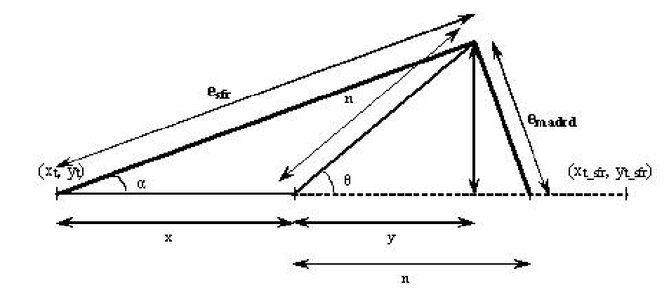

Now consider the node taking the deviation of degrees. Let the distance at which the node takes the deviation be meters after the localization point . The time at which the deviation occurs is greater than time and lesser than . Figure 2 shows the movement of the node. The distance signifies the distance covered in time with constant velocity .
The error in localization between time and can be split up into two parts. The first part is error before the deviation occurs (identical to the fixed velocity analysis above) and the second one is after the deviation. Let be any point on the expected line of motion that the node would have travelled if it had not taken the deviation. If the node would have travelled a distance of along expected straight line, it will travel the same distance after deflection because of constant velocity. Let at the point of deviation and increases along the straight line.


5.1.1 SFR protocol
Let the node use SFR protocol for localizing. The the error at point will be the length of line shown in Figure 2. The equation for is given by Equation 2.
| (1) |
| (2) |
Figure 3 shows the graph of error against . As increases from to , the varies as shown in the graph in Figure 3. We can see that for , the curve is not linear. This can be seen clearly in the case where .
As the angle of deflection increases from to , the error in SFR decreases because the line of motion will be nearer to when increases. For angles greater than and lesser than . The error decreases as node moves towards and then starts increasing.
At , the error touches zero after the node has covered distance and then the error starts increasing linearly. Now the error vector is in other direction than the earlier error vector. Graph in Figure 3 shows the absolute value of the error.
5.1.2 MADRD protocol
| (3) |
The length of the line in Figure 2 shows the the error in MADRD protocol. It increases linearly as the increases. This is given by the equation 3. Graph in Figure 3 shows the comparison of MADRD protocol with SFR for different angles. We observe for acute angles, MADRD protocol performs better than the SFR. However, if is between and , SFR starts performing better. This is because the node is moving away from the predicted motion line and is smaller than the .
5.2 Pause Scenario
In this case, the node comes to a standstill after being in motion with velocity . Let the distance at which the node stops be meters after the localization point , but before the next localization point. In this case, the error in SFR increases linearly until , when it stops increasing. Conversely, the error in MADRD starts at 0 while the node maintains the speed of . However, when it stops moving, the error in MADRD starts increasing proprtionately to since the predictor assumes that the node continues in motion. Interestingly, if the node is standstill but suddenly starts moving with velocity , SFR and MADRD will behave identically until the next localization point (which may be different for each). The reason is that SFR’s uses the implicit prediction that the node remains at the point of the last localization. In this scenario, MADRD uses the same predictor since the node actually was not moving at the last localization point.
Figure 4(a) shows the behavior of MADRD when a turn occurs. In this case, the MADRD estimate continues predicting motion in the original direction. Moreover, even when localization occurs, the average velocity computed as a predictor for the next period will be off as well (it represents the weighted average of the original as well as the new velocities). A similar trend is observed in Figure 4(b) where a node pauses after being in motion at a constant velocity. In this case, the MADRD estimate overshoots the node along the old trajectory when it pauses.
6 Experimental Results
In this section we present the results of our experiments with the proposed protocols. In order to analyze the protocols, we use the ns-2 discrete event simulator [9]. We use a simulation area of 300 by 300 meters, with sensor transmission range of 100 meters using IEEE 802.11. We use 36 equally spaced beacon nodes for localization and 24 mobile nodes carrying out localization. Each simulation was run for 900 seconds. We use a query based localization mechanism: a node that is interested in localization broadcasts a request – beacons that receive the request reply with their location which can then be used to triangulate the nodes own location. The beacons are placed such that at least three, and sometimes four, beacons are able to answer each query. Please note that our results are not dependent on this localization model: we measure the energy in terms of number of localization operations, regardless of how the localization is carried out.


The assumed mobility model has significant implications on the performance of the localization protocols.
We consider first the random waypoint model, widely used in the mobile ad hoc network community. In this model, a node picks a random location in the simulated area and starts moving to it with a controllable average velocity. When the node reaches the destination, it pauses for some fixed pause time. The model is predictable while the node is moving, or for the duration of the pause but not during the period where it pauses or when it starts moving. Further, if the pause time is zero, the model is unpredictable when the node reaches its destination, then picks another randomly and starts moving towards it. We can control how predictable the model is by manipulating the average speed and the pause time – if the pause times are short, the node has more unpredictable behavior. Finally, we present some limited results with Gaussian Markovian mobility pattern which does not lend itself well to prediction using a constant velocity model as we do in MADRD. We used BonnMotion tool [2] to generate the various scenarios.
Figure 5 shows the Instantaneous error for random way-point mobility model with speed uniformly distributed between 4-5 m/sec. The SFR period in this case was chosen to be 2 seconds – the node invokes localization once every two seconds. Note that in the case of SFR and DVM the node assumes that the last measured localization point is its current location. Therefore continues to grow between two successive localization points as the node moves away from its last localization point. Figure 5 shows the instantenous error for SFR, DVM and MADRD protocols. In the case of SFR, sensor 0 localizes approximately at times 0.6, 2.6. As one can see upon localization the error lies within the localization mechanism error range (which we picked to be uniformly distributed between 0 to 0.5 meters). In between the two localization points, the error increases linearly up to 8 meters. In the case of DVM, a similar trend is seen again, howerver due to adaptive localization intervals, the magnitude of the error is lower than that of SFR; DVM was able to discover that it needs to localize more often than once every 2 seconds. In the case of MADRD protocol, the ability to predict the current location gives rise to very low error since the node actually follows the prediction. This graph clearly shows the strength of dead-reckoning procotols due to their prediction capability.


Figures 6(a), 6(b) and 7 show the number of localization operations for three different average velocities normalized to the number needed by SFR. The number of localization operations correlates directly with localization energy since the average cost of localization is constant for most localization schemes. This fact is highlighted in Figure 8 which shows the energy expenditure for the same scenarios as in Figure 7 – the shapes of the figures are very similar. In the case of low mobility 6(a), DVM and MADRD localize less often than SFR. However, as the speed increases, the energy expeniture of DVM and MADRD grow more than that of SFR. Note that since these protocols are adaptive, even for high speeds they adapt well with the increase in pause time thereby spending less energy than SFR when pause time is high.


Figure 9(a) shows the absolute error as a function of mobility for the four protocols for two different pause time values. The primary observation here is that the error for SFR grows linearly with the average velocity while both DVM and MADRD manage to adapt their localization and maintain an error that does not grow significantly with the velocity. Note that under high mobility, this requires more localization operations than SFR as was reflected in the localization frequency diagram for high speeds and low pause time. Figure 9(b) shows the effect of pause time for one velocity. Since pauses affect the prediction of DVM and MADRD, their advantage in terms of error relative to SFR is highest with no pause time. At very high pause times, all three protocols perform well. An alternative measure of localization effectiveness is to monitor the fraction of the simulation time where the localization estimate was within an application specified threshold (in this case 5 meters). Figure 9(c) shows the accuracy as a function of mobility for two pause times. Again, the same trend observed in error is observed here – DVM and MADRD perform much better than SFR, especially as mobility grows. Figure 9(d) shows the accuracy for one average velocity as the pause time is varied.


Recall that to protect against inaccuracies in the prediction model or unexpected changes in the mobility model MADRD must limit the maximum period between localizations (upper query threshold). Figure 10 shows the effect of this tradeoff – we vary the upper query threshold and observe the effect on the accuracy, error and localization energy. If the threshold is raised, this allows MADRD to aggressively predict location without forcing localization operations to ensure that the predictions are accurate. Thus, at high thresholds, higher energy savings are possible, but the expected error grows. A good value for the upper threshold must balance these two effects. Finally, we can use backtracking as explained in the protocol section to recover from some erroneous localizaiton estimates.


Finally, in Figure 11(a) and Figure 11(b) we evaluate the algorithms using the Gaussian mobility model from an energy and error perspective. The Gaussian model is quite different from the assumed monotonic velocity model that underlies both DVM and MADRD; thus, this represents one of the worst case scenarios for these protocols. Nonetheless, they continue to perform comparably to SFR (better in most cases), even for this inappropriate mobility model. In practice, we expect each node to have multiple predictors and continue to score them. At each time, the predictor which has recently been scoring highest would be used to generate the next localization period.
7 Concluding Remarks
In this paper, we explored approaches and tradeoffs to the problem of dynamically managing the Localization period for mobile devices. Localization has several applications both in Sensor Networks and Mobile Ad hoc Networks; for example, accurate localization is necessary to effectively interpret sensor data collected by mobile sensors. A basic localization scheme would simply localize periodically, with a fixed period. However, since the period is not sensitive to the actual mobility of the node, the selected period may be too agressive (wasteful) or insufficient to localize accurately.
We explored two algorithms for dynamic localization: (1) DVM: an adaptive algorithm that matches the localization period to the observed velocity of the node; and (2) MADRD: a predictive algorithm that uses dead reckoning to estimate the location of a node assuming it is following its recently tracked tracjectory. We characterized the performacne of these algorithms for two mobility patterns under different velocities and pause times. Both proposed approaches significantly outperform static localization both from an energy and accuracy perspectives. In particular, MADRD performance was excellent in almost all situations that were studied; however, it is best suited to mobility patterns that are predictable and this result may not generalize to other mobility scenarios.
In all three types of protocols, especially the adaptive and predictive ones, unexpected mobility behavior of the nodes can cause erroneous localization. If such situations are to be minimized, highly aggressive (and inefficient) localization would be needed. Conversely, if some errors can be tolerated, we can adapt the localization period more aggressively resulting in significant energy savings. We propose a technique called backtracking to allow temporary recovery from errors. Specifically, once localization is carried out we may discover that the measured location is far from the expected one. In this case, it is possible to update the location estimate after the fact (e.g., using linear interpolation between the last two points). This is straightforward for samples that have not been sent yet. However, for data that has already been sent, this requires sending a correction signal. Since this signal costs energy, we should still strive to minimize the amount of backtracking needed by the protocols. Another future approach to address the same problem is to use feedback from motion sensors (e.g., an accelerometer). If such a device is available, it can be used to interrupt the primary protocol when a change in the mobility pattern is suspected, causing it to drop back to training mode to capture the new mobility pattern.
In the future we would like to implement these protocols on existing sensor prototypes (eg. Motes) and study their performance. The Zebranet project has developed a simulator for studying systems tradeoffs in wild-life tracking environment in a realistic setting. We would like to port our protocols from ns-2 to ZNetSim [5] and study the performance for an existing application. At present our work is limited to individual mobility models; but in the future we will also explore group mobility models. For military scenarios for example we can imagine a group of soldiers moving together to achieve certain goal. We would like to evaluate the protocols proposed in this paper for such scenarios and suggest some improvements.
References
- [1] Bahl, P., and Padmanabhan, V. N. RADAR: An in-building RF-based user location and tracking system. In INFOCOM (2) (2000), pp. 775–784.
- [2] BonnMotion. http://web.informatik.uni-bonn.de/IV/Mitarbeiter/dewaal/BonnMotion/.
- [3] Bulusu, N., Heidemann, J., and Estrin, D. Gps-less low cost outdoor localization for very small devices. IEEE Personal Communications Magazine 7, 5 (October 2000).
- [4] He, T., Huang, C., Blum, B. M., Stankovic, J. A., and Abdelzaher, T. Range-free localization schemes for large scale sensor networks. In Proceedings of the 9th annual international conference on Mobile computing and networking (2003), ACM Press, pp. 81–95.
- [5] Juang, P., Oki, H., Wang, Y., Martonosi, M., Peh, L. S., and Rubenstein, D. Energy-efficient computing for wildlife tracking: design tradeoffs and early experiences with zebranet. In Tenth international conference on architectural support for programming languages and operating systems on Proceedings of the 10th international conference on architectural support for programming languages and operating systems (ASPLOS-X) (2002), ACM Press, pp. 96–107.
- [6] Ko, Y.-B., and Vaidya, N. H. Location-aided routing (lar) in mobile ad hoc networks. In Proceedings of the 4th annual ACM/IEEE international conference on Mobile computing and networking (1998), ACM Press, pp. 66–75.
- [7] Kumar, V., and Das, S. R. Performance of dead reckoning-based location service for mobile ad hoc networks. Wireless Communications and Mobile Computing Journal (to appear) (Dec 2003).
- [8] Niculescu, D., and Nath, B. Ad hoc positioning system (aps) using aoa. In In Proceedings of INFOCOM (2003).
- [9] Network Simulator. http://isi.edu/nsnam/ns.
- [10] Priyantha, N. B., Chakraborty, A., and Balakrishnan, H. The cricket location-support system. In Mobile Computing and Networking (2000).
- [11] Savvides, A., Han, C.-C., and Strivastava, M. B. Dynamic fine-grained localization in ad-hoc networks of sensors. In Proceedings of the 7th annual international conference on Mobile computing and networking (2001), ACM Press, pp. 166–179.
- [12] Ward, A., Jones, A., and Hopper, A. A new location technique for the active office. In IEEE Personnel Communications (1997).