Non-uniform Information Dissemination for Sensor NetworksThanks: An earlier version of this paper appeared in the International Conference on Networking Protocols (ICNP 2003) [15]. Significant changes in this paper include the addition of an analysis of the protocol in the presence of mobility, as well as an expanded discussion section.

Sameer Tilak^†, Amy Murphy^‡, Wendi Heinzelman^‡ and Nael B. Abu-Ghazaleh^†

^†Computer System Research Laboratory Dept. of CS, Binghamton University Binghamton, NY 13902–6000 {sameer,nael}@cs.binghamton.edu ^‡Computer Science Department University of Rochester Rochester, NY 14627–0126 {murphy,wheinzel}@cs.rochester.edu

Abstract

Future smart environments will be characterized by multiple nodes that sense, collect, and disseminate information about environmental phenomena through a wireless network. In this paper, we define a set of applications that require a new form of distributed knowledge about the environment, referred to as non-uniform information granularity. By non-uniform information granularity we mean that the required accuracy or precision of information is proportional to the distance between a source node (information producer) and current sink node (information consumer). That is, as the distance between the source node and sink node increases, loss in information precision is acceptable. Applications that can benefit from this type of knowledge range from battlefield scenarios to rescue operations. The main objectives of this paper are two-fold: first, we will precisely define non-uniform information granularity, and second, we will describe different protocols that achieve non-uniform information dissemination and analyze these protocols based on complexity, energy consumption, and accuracy of information.

1 Introduction

Smart environments are characterized by a large number of distributed sensors that collect environmental information and disseminate that information across wireless links. Typically, sensor networks focus on collecting this information in a single place for analysis, taking into consideration optimizations from local aggregation (e.g., LEACH [5]) or processing data en route to a central location (e.g., MagnetOS [12]). While such central collection is important for many applications, it does not match the requirements of all applications that can exploit sensor networks.

For example, consider a military application with sensors distributed throughout an area collecting information about passing vehicles, air contaminants, land mines, and other environmental data. We assume the sensors can communicate with one another, and a soldier that moves throughout the region can contact any nearby sensor to find out both the state of that sensor, as well as any other information it has collected from the other networked sensors. For this soldier, clearly the events occurring in the immediate neighborhood are most important. For example, it is more critical to know about a land mine nearby than one several miles away. Nonetheless, it is still important that the soldier have a general overview of the area in order to plan and make appropriate decisions. Similarly, consider a rescue scenario where a team of fire fighters is working to rescue trapped victims. In this case, the fire fighters require precise information about their immediate surroundings in order to make decisions about using resources to make progress, as well as some global knowledge to plan a path to the victims as well as an escape path back to safety. In the above applications, sensors are static and mobile users connect to the nearby sensors to obtain the required information. However, one can imagine a network where mobile users themselves are carrying sensors placed on them. In this paper, we focus on protocols for static sensor networks (sensors are stationary), but then show that the protocols are resilient to mobility.

The applications above differ from those typically studied for sensor network applications in the following way: the information is not collected centrally, but instead it is utilized at several places in the network (e.g., the locations of the individuals). While some sensor network applications accomplish this in a query driven manner, asking a central source for the latest collected information, these applications require continuous updates. A simplistic solution to this problem is to proactively flood updates from each sensor to every other sensor. This solution is extremely inefficient and does not scale to large numbers of sensors. In the scenarios we target, information from a particular sensor is most important to those surrounding it, with the value of the information decreasing as a function of distance from the sensor. Specifically, the necessary precision of information is proportional to the distance between an information producer and an information consumer. We refer to such a requirement as a non-uniform information dissemination requirement, a new concept we introduce here.

This paper introduces and analyzes several protocols that perform non-uniform information dissemination. As these protocols are intended to run on wireless sensor networks, they must abide by the requirements of that environment, namely they must be energy efficient and have low complexity. The distinguishing feature of this new application class is that it is possible to trade accuracy of disseminated information for energy. Our experimental results clearly show this trade-off using a number of different protocols.

The remainder of this paper begins with a characterization of the requirements for non-uniform information dissemination protocols. Section 3 describes the details of several protocols. In section 4, we discuss the implementation details of the protocols within the ns-2 simulator and then present our experimental results, followed by a discussion in section 5, which presents more insight into our results. Section 6 describes related work and section 7 presents conclusions and future work.

2 Design Goals

We propose using the following design goals for sensor network protocols for applications that have non-uniform information dissemination requirements.

•

Energy efficiency. As sensor nodes are battery-operated, protocols must be energy-efficient to maximize system lifetime.
•

Accuracy. Accuracy is a measure of the sensing fidelity: obtaining accurate information is the primary objective of a sensor network. Accuracy is a metric that is application-specific both in terms of the appropriate metric and the required fidelity level. There is a trade-off between accuracy, latency and energy efficiency. In the applications we target, it is acceptable for sensors to have information with low accuracy about locations that are far away, but they should have highly accurate information about locations that are close by. Because of this non-uniform information dissemination requirement, a given sensor will not have all the information from all other sensors at every point in time. Consider a case where sensor $S_{1}$ receives every $n^{th}$ packet from another sensor $S_{2}$ . In this case, $S_{1}$ receives the $i^{th}$ packet from $S_{2}$ at time $t_{1}$ and the $(i+n)^{th}$ packet from $S_{2}$ at time $t_{2}$ , ( $n>1$ ). Thus, in the interval ( $t_{1}$ , $t_{2}$ ), the information $S_{1}$ has about $S_{2}$ is not as accurate as a sensor that receives every update that $S_{2}$ sends. We define accuracy in terms of the difference between the local value of the information and the actual value.
•

Scalability. Scalability for sensor networks is also a critical factor. For large-scale networks, distributed protocols are needed such that the protocol is based on localized interactions and does not need global knowledge such as the current network topology.

With these design goals in mind, in this paper we present simple deterministic protocols (Filtercast and RFiltercast) and non-deterministic protocols (unbiased and biased protocols) to achieve non-uniform information dissemination. Compared to flooding, these protocols reduce the cost of communication by reducing the number of packet transmissions and receptions. At the same time, these protocols are designed to operate within the application-specific tolerance in terms of accuracy. Our results indicate that these protocols outperform flooding in terms of energy efficiency by trading-off accuracy for energy while keeping the accuracy acceptable by the application. The next section describes the details of each of these protocols.

3 Dissemination Protocols

This section introduces the mechanisms of several protocols that perform non-uniform information dissemination. Similar to traditional sensor networks, every sensor in the network serves as a source of information to be spread throughout the network. Unlike traditional networks where a specific node serves as the sink node, every sensor in our system receives and stores some data from the other sensors in the system.

We begin our protocol discussion with a traditional flooding algorithm. Flooding achieves uniform information dissemination, and serves as a baseline of comparison for the rest of our protocols. Following this, we introduce two new deterministic protocols and analyze two non-deterministic protocols [13].

3.1 Traditional Flooding

In flooding, a sensor broadcasts its data, and this is received by all of its neighbors. Each of these neighbor sensors rebroadcasts the data, and eventually each sensor in the network receives the data. Some memory of packets is retained at each sensor to ensure that the same packet is not rebroadcast more than once. If each sensor broadcasts its data, then with this flooding protocol, every sensor in the network will receive data from every other sensor. Thus, ignoring distribution latency, which is the amount of time required for a packet to travel from the source to the farthest sensor in the network, every sensor has an identical view of the network at every point in time (ignoring packet collisions and timing issues). Furthermore, the protocol itself is simple and straightforward to implement. Unfortunately the simplicity and high accuracy come at the price of high energy expenditure. The massive data replication requires active participation from every sensor in the network, and thus sensors can quickly run out of energy.

3.2 Deterministic Protocols

In analyzing the flooding algorithm, it is apparent that to achieve non-uniform information dissemination, one approach is to simply have intermediate nodes forward fewer packets. The two protocols we introduce here, Filtercast and RFiltercast, achieve just that by deterministic means.

3.2.1 Filtercast

As the name suggests, Filtercast filters information at each sensor and does not transmit all the information received from other sensors in the network. Filtercast is based on a simple idea of sampling information received from a given source at a certain rate $n$ , specified as a parameter to the protocol. The lower the value of $n$ , the more accurate the information disseminated by the protocol. When $n=1$ , Filtercast behaves identically to flooding. During protocol operation, each sensor keeps a count of the total number of packets it has received so far from each source, $source_{cnt}$ . A sensor forwards a packet that it receives from $source$ only if $(source_{cnt}\;mod\;n)==0$ , then increments $source_{cnt}$ . We refer to the constant $\frac{1}{n}$ as the filtering frequency. The intuition behind this protocol is that as the hop count between a source node and a sink node increases, the amount of information re-transmitted decreases due to the cascading effect of the filtering frequency at each subsequent sensor.

While this reduces the total number of transmissions compared to flooding, the state information maintained at each sensor increases. Specifically, each sensor must maintain a list of all the sources it has encountered from the start of the application and a count of the number of packets seen from each of these sources. As this increases linearly with the size of the network, it may pose some scalability problems.

3.2.2 RFiltercast

One potential problem with Filtercast is the synchronization of the packets transmitted by the neighbors. For example, consider a scenario where sensors $s_{2}$ and $s_{3}$ are one-hop neighbors of both $s_{1}$ and $s_{4}$ , while $s_{1}$ and $s_{4}$ are two hops away from each other. In this case, if Filtercast is used as a dissemination protocol, then $s_{2}$ and $s_{3}$ will end up forwarding either all odd or all even packets (synchronized on forwarding the packets) from $s_{1}$ to $s_{4}$ , effectively transmitting redundant information.

Our intuition is that if we can remove this redundancy, we may be able to increase the accuracy of the protocol without increasing the energy expended.

To address this effect, we propose another protocol: Randomized Filtercast (RFiltercast). In this variant of Filtercast, the filtering frequency $\frac{1}{n}$ is still the same for all sensors, but each sensor generates a random number $r$ between $1\ldots n$ and re-transmits a packet if $(source_{cnt}\;mod\;n)-r==0$ . Intuitively, this means that each sensor considers a window of size $n$ and will transmit only one of the packets from a given source in this window. So, for a window of size $2$ , half of the packets will be selected for re-transmission, but instead of always re-transmitting the first of the two packets (as in Filtercast), the sensors that choose $r=1$ will transmit the first of the two packets while the sensors that choose $r=2$ will transmit the second of the two packets.

While our intuition was that the same energy would be expended by RFiltercast as for Filtercast, this turns out not to be true. In fact, RFiltercast transmits more packets than Filtercast, but fewer than Flooding, putting its energy expenditure in between the two. This effect happens because in RFiltercast, a node receives more packets from a given source, as described above, and thereby ends up transmitting more packets on behalf of the source. Note that forwarding decisions at an intermediate node are not based on packet IDs but are based on the number of unique packets received from the source node. Therefore, due to the reception and transmission of more packets in RFiltercast, the energy dissipation of RFiltercast is higher than that of Filtercast.

While RFiltercast has more transmissions, increasing its energy expenditure, it also has improved accuracy over Filtercast. The crucial point to extract is that RFiltercast should, on average, propagate information faster than Filtercast, leading to more accurate data throughout the network, but RFiltercast will require less energy than flooding.

3.3 Randomized Protocols

Both RFiltercast and Filtercast are lightweight and easy to analyze due to their deterministic nature. However, they still have some overhead in terms of the state required at each node.

We next describe several probabilistic protocols. In these protocols, when a sensor receives a packet, it chooses a random number and then decides whether to forward the packet or not based on the number chosen. We classify these protocols into two categories: biased and unbiased protocols. In the biased protocol, sensors bias their decision about whether to forward a packet based on the location of the source, where packets from close sensors are more likely to be forwarded than packets from distant sensors. In the unbiased protocol, all packets are forwarded with equal probability.

3.3.1 Unbiased Protocol

The notion of using probabilities to flood packets throughout a network has been studied previously [1, 6, 11, 17], but to the best of our knowledge, no studies exist that explore its applicability to non-uniform information granularity requirements. Similar to the deterministic protocols, the unbiased protocol also takes a parameter that affects the accuracy of the forwarding. In this case, the parameter specifies the probability that a packet should be forwarded. In the case of the unbiased protocol, this value is the same for each incoming packet.

The main advantage of this protocol is its simplicity and low overhead. As every packet is forwarded only with a certain probability, the protocol results in less communication compared to flooding (proportional to the forwarding probability). Also, the protocol does not require state to be kept, giving this protocol the potential to scale well.

To adjust the accuracy of the information throughout the network, the forwarding probability can be tuned according to the application needs. The primary tradeoff, however, is energy for accuracy. In general, as the forwarding probability increases, the behavior converges toward flooding. While our current study considers only constant probabilities, in the future we will look at the possibility of probabilities being adjusted dynamically to adapt to the current network traffic and the application needs.

3.3.2 Biased Protocol

In this protocol, the forwarding probability is chosen to be inversely proportional to the distance the packet has traveled since leaving the source sensor. In other words, if a sensor receives a packet from a close neighbor, it is more likely to forward this than a packet received from a neighbor much farther away. To estimate distance between sensors, a sensor examines the TTL (time-to-live) field contained in the packet. If we assume all sensors use the same initial TTL, we can use the current TTL to adjust the forwarding probability for each packet. The following tuples indicate the forwarding probabilities used (second number in the tuple) when the packet has traveled the number of hops in the range specified in the first part of the tuple: $<1-3,~0.8>$ , $<4-6,~0.6>$ , $<7-9,~0.4>$ , $<10+,~0.2>$ .

Using TTL to estimate distance is simple; however, note that TTL does not always indicate the exact distance between two sensors. For example, consider a source node $S$ and a destination node $D$ . It is possible that either due to congestion or collisions, a packet gets dropped along the shortest path and another packet reaches node $D$ via a longer route. In that case, the TTL would give a false estimate of distance. However, in a static network, node $D$ can always maintain its current estimate of the TTL to node $S$ . In the case of mobile sensors, as the distance between $S$ and $D$ changes (decreasing, for example, as the nodes get closer), this is reflected in the subsequent packets (higher TTL value) and thus node $D$ gets more and more accurate information about $S$ . We use the TTL-based approach for the biased protocol mainly for its simplicity, resilience to mobility and energy efficiency.

Similar to the unbiased protocol, this biased protocol requires no additional storage overhead unless node distances are stored, and the protocol itself is completely stateless (note, however, that this does not eliminate the caching of recently seen packets in order to avoid re-broadcasting the same packet multiple times). Therefore, this protocol scales as well.

4 Experimental Study

In order to analyze the protocols, we use the ns-2 discrete event simulator [10]. Table 1 lists the relevant parameters used during our simulations.

Table 1: Simulation parameters.

Simulation area	$800\times 800~m^{2}$
Transmission range	$100~m$
Initial Energy	$10000~J$
MAC Protocol	$802.11$
Bandwidth	$1~Mbps$
Transmit Power	$0.660~W$
Receive Power	$0.395~W$
Idle Power	$0.0~W$
Number of Nodes	$100$

In the case of static networks, we consider two sensor deployment strategies: uniform and random. In a uniform deployment strategy, sensors are distributed with some regular geometric topology (e.g., a grid). With random deployment, sensors are scattered throughout the field with uniform probability. For a battlefield-like scenario, random deployment might be the only option, but with applications such as animal tracking in a forest, sensors may be deployed in a deliberate, uniform fashion.

In order to simulate sensor readings, we divide the simulation into an initialization phase and a reporting phase. During the initialization phase, each sensor chooses a random number between $0$ and $100$ to serve as its initial sensor reading. During the reporting phase, each sensor increments its reading by a fixed amount at fixed intervals. In the real world, due to correlation among physically co-located sensors, sensors will have a different reading pattern; however, this simulation does provide us with valuable information about the behavior of our protocols under various conditions. In the latter part of this section, we present a revised data model that tries to capture correlation among sensor readings. Our results indicate that the overall behavior of the protocols shows a very similar trend for both data models.

4.1 Traffic Load Study

This study focuses on evaluating the effect of a change in traffic load for both grid and random topologies. In the first set of experiments, we study the effect of varying traffic loads systematically from $5$ packets/sec to $1$ packet/ $2$ sec. The goal of these experiments is to understand the relationship between accuracy, reporting rate, and network capacity for both uniform and non-uniform dissemination scenarios.

Note that in order to calculate accuracy, we find the difference between a sensor’s local view of another sensor’s data and the actual value of that sensor’s data. A view is essentially the latest data that one sensor has from another sensor. This view is then normalized based on distance. Let $R(S_{i,j})$ denote sensor $S_{i}$ ’s view of sensor ${S_{j}}$ ’s data, and let $n$ be the total number of sensors in the network. The weighted error $e_{i}$ for a sensor $S_{i}$ is given as:

e_{i}=\frac{1}{n}\,\Sigma_{j=1,j\neq i}^{n}|(R(S_{i,j})-R(S_{j,j})|*\,w_{ij}

(1)

w_{ij}=\frac{1}{\frac{\lceil d(S_{i},S_{j})\rceil}{\gamma}}

(2)

where $d(S_{i},S_{j})$ is the Euclidean distance between sensors $S_{i}$ and $S_{j}$ and $\gamma$ was set to 100 (the transmission range of each node). The fist equation shows that for a given sensor we calculate weighted average error with respect to all other sensors in the network. We vary the weight in terms of distance with a step size of 100 meters.

Note that Euclidean distance is used as the weighing factor so that the higher the distance, the smaller the contribution of error toward overall error. This error calculation describes our non-uniform data dissemination requirement by giving higher weight to errors for data that originated in a close neighborhood and lower weight to errors for data that originated from a distant sensor. It is worth noting that although we refer to this as error, because the value of the data at the source increases linearly, it also represents the accuracy of the data.

Our results indicate that with flooding, congestion is a severe problem, and other protocols are less prone to the congestion problem. In this type of application, the effect of congestion is worse than that observed in traditional sensor networks [14]. From the simulation studies, we can see that flooding is the least energy-efficient protocol and has the highest error if the network is congested. RFiltercast and the biased protocol are more energy-efficient than flooding and provide low error in most cases. Filtercast and the unbiased protocol are the most energy-efficient protocols, but their accuracy is good (low error) only at higher sending frequencies.

4.1.1 Grid Topology

Figure 1 shows the performance of flooding, Filtercast, RFiltercast, and the biased and unbiased randomized protocols under various traffic loads for the grid topology. In these graphs, distance is varied across the X-axis (in steps of 100 meters) and the Y-axis shows mean unweighted error (mean absolute error). Note that, with non-uniform information dissemination, as the distance between the source node and sink node increases, loss in information precision is acceptable.

From Figure 1(a), where the data rate is $5$ packets/sec, we can see that even though theoretically flooding should have no error, due to congestion, flooding has the highest error. This is due to the fact that if the total traffic exceeds the network capacity, congestion causes packets to be dropped and this gives rise to loss of information and high error. At the same time, high traffic results in higher collisions. In this situation, even RFiltercast and the biased randomized protocol result in high traffic load and thus they have high error as well. However, both Filtercast and the unbiased randomized protocol (with forwarding probability of 0.5) perform well in this case because the traffic load does not exceed the available network capacity. As expected, for all protocols the error increases as the distance from the source increases, resulting in non-uniform information across the network.

Refer to caption — (a) Data rate 5 packets/sec.

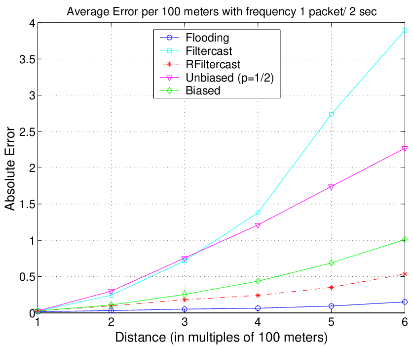
When the sending frequency is changed to $2$ packets/sec, as shown in Figure 1(b), flooding the network still causes congestion and thus flooding has high error. However, now for both RFiltercast and the biased protocol, the load does not exceed the network capacity and their performance is better than in the previous case. Also, note that now these two protocols perform better in terms of error rate than the unbiased protocol and Filtercast because of the fact that they disseminate more information yet the information disseminated does not exceed the network capacity.

When the sending frequency is lowered to $1$ packet/sec, as shown in Figure 1(c), then even flooding does not exceed network capacity. Since the network is no longer a bottleneck, flooding disseminates the maximum information successfully and clearly has the lowest error. Both the biased and RFiltercast protocols perform better than the unbiased protocol and Filtercast. The unbiased protocol and Filtercast have the highest error in this case because they do not disseminate as much information as the other protocols. The same trend continues even for the lowest sending frequency, shown in Figure 1(d).

The interesting point about these results is the oscillatory behavior of the energy-error curves. To elaborate further on this, if the total data exceeds network capacity, then any further data on the channel will increase congestion and decrease overall lifetime of the network. When the amount of data transmitted is below network capacity, then there is a trade-off between energy spent and accuracy observed. This is because as long as the total data does not exceed network capacity, sending more data will improve accuracy at the cost of energy spent in communication. However, with non-uniform information granularity, accuracy between two sensors is proportional to distance between them. Therefore, RFiltercast and Filtercast try to achieve this by filtering packets and the randomized protocols try to achieve this by probabilistically forwarding packets.

Figure 2 shows the trade-off between energy and weighted error, using the weighted error calculation method described in Eqns. 1 and 2. In Figure 2, the X-axis indicates the energy spent in Joules and the Y-axis shows mean weighted error. Each point represents one of the sending frequencies, ranging from 5 packets per second for the left-most point of each curve to one packet per two seconds for the right-most.

For flooding, when the reporting frequency is highest, the energy spent is maximum. However, as mentioned earlier, congestion and collisions cause high error. As the sending frequency decreases to the point that total traffic does not exceed network capacity, the error also decreases. Flooding performs the best in terms of accuracy (minimum error) when the sending frequency is $1$ packet/sec; after this rate, the error starts increasing due to the fact that not enough information is propagated. This is an interesting phenomenon, where the error oscillates between these two bounds. The upper bound is a function of the network capacity, whereas the lower bound is a function of the application-specific accuracy. Previous research has also shown this phenomenon [14].

Based on the energy-error trade-off, we can say that at high sending frequency, flooding performs the worst by spending high energy while not providing accurate information (high error). RFiltercast and the biased protocol start performing better than flooding at high rates. There is a considerable difference between energy and error for RFiltercast and the biased protocol compared to flooding at the sending frequency of $2$ packets/sec. As one can anticipate, flooding performs better than all other protocols in terms of accuracy when the sending frequency is $1$ packet/sec, but note that there is not much difference between flooding, RFiltercast and the biased protocol even when the network is operating in the non-congested mode. Filtercast and the unbiased protocol perform best in terms of energy and error at high sending frequencies and their performance relative to the other protocols starts to degrade as the sending frequency is reduced.

The desirable mode of operation for a protocol is in the region where minimum energy is spent and low error is observed. Note that the desired mode of operation for a protocol depends on factors such as network density, transmission range of the radios, etc. In our future work, we will perform an analytical study to address this issue. From Figure 2, this zone lies around sending frequency $2$ packets/sec to $1$ packet/sec for RFiltercast and the biased protocol, whereas for flooding it lies at sending frequency $1$ packet/sec. We want to point out that as the network size increases, flooding can pose severe problems in terms of scalability and energy efficiency. Therefore, randomized protocols should be considered as viable alternatives in these cases. In our experiments we had a network of 100 sensors, but with a network of thousands of sensors we believe that randomized protocols will perform much better than flooding. With randomized protocols, the biased protocol performs the best by spending moderate energy and getting high accuracy.

Our results show that randomized protocols can achieve high energy savings while at the same time achieving acceptable accuracy with almost no overhead. Also note that RFiltercast and the biased protocol have almost equivalent error curves while the biased protocol has negligible overhead.

4.1.2 Random Topology

Figure 3 shows our results with a random topology and the same traffic loads as before. The results for 1 and 2 packets/sec and the energy tradeoff study show expected results similar to those achieved for the grid topology, and are therefore not shown here. It is not clear whether regular deployment will offer advantages over uniformly distributed random deployment; if it does not, random deployment is preferable because of its low cost.

4.1.3 Transmission Range

Our next set of experiments show the effect of an increase in the transmission range from the original 100 meters to 150 meters, while keeping the original 10x10 grid topology. An increase in transmission range corresponds to an increase in the degree (connectivity) of a sensor. This results in decreasing the capacity of the network, meaning congestion occurs even at low sending frequencies. Intuitively, this will make the overall situation worse if the network is operating in a congested mode. This can be seen from our results, comparing Figures 1(a) and 4(a), as there is an increase in overall error for flooding, RFiltercast and the randomized protocols.

In this case, even at the low sending frequency of $1$ packet/sec shown in Figure 4(c), flooding does not perform well due to network congestion. Previously, when the transmission range was $100$ meters, flooding performed well at this sending frequency (see Figure 1(c)). However, when the network is not congested, then due to the higher connectivity and shorter average hop length, the average error decreases. For example, for RFiltercast and the biased protocol, when the sending frequency is $1$ packet/sec, then the maximum absolute error values with a transmission range of $100$ meters are $0.4$ and $0.6$ respectively, as shown in Figure 1(c). With the transmission range changed to $150$ meters, Figure 4(c) shows that the maximum absolute error for RFiltercast and the biased protocol changes to $0.24$ for both.

Similarly, all the protocols have low error values at a sending frequency of $1$ packet/ $2$ sec when the transmission range is $150$ meters, as shown in Figure 4(d), compared to the simulations with $100$ meters transmission range, shown in Figure 1(d).

Up to this point our study considered static networks. In the next subsection we analyze protocols for non-uniform information dissemination in the presence of mobility along with a revised data model.

4.2 Mobility Study

To motivate the case for mobile sensors, consider a battlefield scenario, where soldiers and armed vehicles are moving carrying tiny sensors along with them. Each sensor is collecting information about air contaminants so as to find out about potential biological/chemical attacks. In this case as a soldier moves around, the presence of an air contaminant sensed by the sensor changes depending upon the sensor’s current location in the battlefield. Also, for a small change in location, there is not a very high change in the percentage of contaminant reported. We can think of this as a spatio-temporal process, where there is both spatial and temporal correlation among the readings reported by the sensors. This means that correlation among the sensor readings is a function of the distance between them; the closer the sensors are, the higher the correlation between their data.

In order to model this application, we divide the simulation area of $800$ x $800$ meters into 16 squares, each called a zone. We assume that the sensor readings (contaminant in this case) follow a normal distribution in space (inter-zonal distribution). For the inter-zonal distribution, we set the mean to 20 and the standard deviation to 2. This corresponds to a loose correlation among data sensed by all the sensors in the battlefield. Also, there will be very high correlation among data reported by sensors within the same zone. We modeled the correlation among sensors within a zone (intra-zonal) to follow a normal distribution but with low variance compared to that of the inter-zonal distribution. For the intra-zonal distribution we set the standard deviation to be a random number in the interval of $0$ to $0.5$ (both inclusive). Also, we vary the mean of the intra-zonal distribution as the simulation progresses to reflect the temporal variations. During the initial half of the simulation, the mean slowly increases and then during the later half of the simulation it decreases gradually. For evaluating the performance of these protocols, we calculate the weighted error in the same way that we did for the static networks (e.g., Eqns. 1 and 2). We want to emphasize that these zones are just an artifact of modeling the phenomenon (contaminant presence across the field).

For static networks, distance between every pair of sensors is fixed (time invariant). However, in the case of mobile sensors, as the sensors move around, the distance between a pair of sensors changes. By non-uniform information granularity, we intuitively mean that a sensor should have very precise information about its local neighborhood and loss in accuracy should be proportional to the distance between source and sink sensors. However, with mobile sensors, as the sensors move, the local neighborhood of a sensor changes as a function of time. It is thus interesting to study how the protocols (both deterministic and randomized) react to these neighborhood changes.

We now analyze the performance of all the protocols when nodes are mobile with the revised data model. For mobility we consider the following two cases. In the first case we set the maximum speed of the sensors to 2 m/s (Figure 5) and in the second case to 10 m/s (Figure 6). The former model represents walking speeds (e.g., soldiers) while the later one represents vehicle speeds (e.g., tanks).

The results presented here are the average of runs over 3 random topologies. The error calculation is done based on the distance between two nodes at the time of reading. Note that for the static network simulations we previously discussed, nodes chose a random number between 0 and 100 as their initial value and then during the reporting phase, each sensor incremented its reading by a fixed amount (10 each second) at fixed intervals. In the revised data model, the variations in the sensor readings are not so high. Thus, the results with the revised data model and the initial data model are not comparable numerically per se. However, one can clearly see the same trend in the relative performance of the different protocols. Figures (5(a) and 5(b)) and (6(a), 6(b), and 6(c)) show that RFiltercast and both the randomized protocols perform better than or very close to that of flooding while the error value for Filtercast is high. Similar to its performance in static networks, for low data rates, flooding starts performing better in terms of accuracy than all the other protocols.

Figure 7 shows the trade-off between energy and weighted error, using the weighted error calculation method described in Eqns. 1 and 2 for both mobility cases. In these figures, the X-axis indicates the energy spent in Joules and the Y-axis shows mean weighted error. The trends observed are very similar to that of the static network (Figure 2). At high data rates, flooding spends maximum energy and has the highest error. Note that for higher mobility (Figure 7(b)), the performance of flooding is worse than that of the low mobility case (Figure 7(a)). In the case of high mobility, the performance of RFiltercast and the biased randomized protocol is better than flooding except for the lowest data rate. These results indicate that the protocols are resilient to mobility, as changes in speed have almost no impact on the error values of the protocols for a realistic data model.

5 Discussion

Overall from these results, we can conclude the following: in the case of applications that can exploit non-uniform information, protocols can be designed to make efficient use of the available bandwidth while providing the necessary level of accuracy. Generally, RFiltercast outperforms Filtercast when the network is not congested. Also, naive, randomized protocols such as the unbiased protocol, outperform specialized protocols such as Filtercast. This is because in general these protocols forward messages more aggressively with the parameters we selected. In our setting, since accuracy is a function of distance, the errors for far sensors count less and thus overall these protocols perform well. The biased randomized protocol has comparable performance to that of RFiltercast.

In the simulations presented here, the biased protocol performs better in terms of accuracy than the unbiased protocol, even for distant sink nodes. This effect is simply due to the forwarding probability settings and, most importantly, the size of the simulated networks, which limits the maximum number of hops between the source and destination. As mentioned previously, in the biased protocol sensors transmit packets from nearby sensors with high probability, and this probability decreases linearly as a function of the number of hops between the source and the sensor transmitting the packet (see section 3.3.2). However, in the case of the unbiased protocol, for any packet that needs to be forwarded, the forwarding probability is constant (0.5 in our simulations). In our simulations, the maximum number of hops is limited to six, since we could not run larger simulations due to computational resource constraints. Therefore, for the simulations presented here, the biased protocol has higher forwarding probability than the unbiased protocol for the first few hops (with respect to the source), which dominates the picture. We conjecture that if we increase the number of hops (to, say, 20), then for distant sinks, the unbiased protocol will perform better than the biased protocol in terms of accuracy. Note that both Filtercast and RFiltercast have some overhead to maintain the source lists and the count of how many packets a given source node has transmitted. On the other hand, the randomized protocols do not require such state to be maintained. Also, the randomized protocols are resilient to mobility. We believe that randomized protocols with intelligent adjustments of forwarding probabilities can be considered as the most efficient alternative for non-uniform data dissemination.

6 Related Work

Recently, sensor networks have drawn a considerable amount of attention from the research community. Most of this existing work focuses on two primary cases: (1) Sensors send their data toward a central base station that has infinite power and is responsible for all data processing, and no in-network processing is done. (2) Sensors do some in-network data processing such as data fusion and this high level data is sent to the central base station. A number of such approaches have been proposed (e.g., [4, 7, 9]). However, in our case, we do not assume the presence of any such base station, and the sensors disseminate information among themselves so that the user can connect to any of the sensors to extract network information.

Other studies considered specific sensor network applications and their implication on protocol design. Cerpa et al. [2], have considered habitat monitoring and have designed protocols to match the application need. Heinzelman et al. [5], described adaptive protocols for information dissemination. In this work, to save energy, sensors send out advertisements for data they have, and they only send the actual data if it is requested by one or more nodes. In previous work [13], we described probabilistic flooding alternatives. However, the main goal of that work was congestion avoidance rather than non-uniform information dissemination.

Li et al. [8] proposed a gossip-based approach for routing protocols to reduce routing overhead. However, the study focused only on routing messages (with implicit uniform information granularity requirement). Recently, Barette et al. [1] proposed a family of gossip-based routing protocols for sensor networks. In their study they considered various parameters such as the number of hops between the source and the destination, the number of hops the packet has traveled, etc.

In the DREAM [11] routing protocol, routing tables are updated based on the distance between two nodes and the mobility rate of a given node. While this work has a similar flavor to our work, exploiting non-uniform information needs, it is limited to only adjusting routing tables and does not apply to the actual data that is exchanged between two nodes.

Kempe et al. [3] presented theoretical results for gossiping protocols with resource location as a motivating problem and delay as the primary consideration. In their setting, a node at distance $d$ from the origin of a new information source should learn about it with a delay that grows slowly with $d$ and independent of network size. They do not consider application level performance criteria such as accuracy, which is part of our study.

In this paper we have considered flooding as one of the alternatives for data dissemination in sensor networks. However, flooding and its alternatives have also been explored in the context of mobile ad hoc networks. Perkins et al. describe IP Flooding in ad-hoc networks [6]. While this paper considers probabilistic flooding protocols for sensor networks, Sasson et al. have studied probabilistic flooding for ad hoc networks [17] and used the phase transition phenomenon as a basis to select the broadcasting probability. Williams et al. [16] described and compared several broadcasting protocols (including probabilistic protocols) in the context of mobile ad hoc networks.

The primary difference between our work and existing work is the application requirement. In our study, we focus on a new application requirement, non-uniform information dissemination, and we analyze protocols for this class of applications.

7 Conclusions and Future Work

In this paper we considered sensor network applications where events need to be disseminated to observers that may be present anywhere in the sensor field. For such applications, simply flooding all the data is extremely wasteful. Therefore, we defined the idea of non-uniform information dissemination to capitalize on the fact that the value of data is typically highest for observers that are closest to the source of the data. We developed and analyzed several protocols to accomplish non-uniform dissemination, both deterministic (Filtercast and RFiltercast) and non-deterministic (unbiased and biased) protocols, and we evaluated them under various traffic loads and transmission ranges and with or without mobility. In all cases, the developed protocols were clearly superior to simple flooding, both from an application and a network perspective. With flooding, congestion appears to be a limiting constraint and further, flooding is not generally energy-efficient. Our results indicate that the performance of RFiltercast and the biased randomized protocol is almost equivalent. RFiltercast requires each sensor to maintain some extra state information, whereas the biased randomized protocol is completely stateless and has negligible overhead. Also, we note that the performance of Filtercast and the unbiased randomized protocol is almost equivalent. We also showed that RFiltercast as well as the randomized protocols are resilient to mobility.

While in this paper the distance between two nodes is used as a parameter for non-uniform data dissemination, in our future work we will focus on a broad range of applications with a non-uniform information dissemination requirement, where factors other than distance, such as importance of the information and confidence in the generated data, can be used. Also, we would like to develop protocols that will tune the forwarding probabilities dynamically depending upon factors such as traffic load, network connectivity, resources (remaining battery power), etc. We believe that this will be an important step towards making these networks self-configuring.

We would also like to develop a priority-based protocol where a source marks all its outgoing packets with a certain priority to indicate the importance of the information contained in the given packet. Any forwarding node can consider the priority of the packet when making its forwarding decision. These techniques will extend the applicability of non-uniform information dissemination to new classes of applications for wireless sensor networks.

References

[1] C. L. Barrett, S. J. Eidenbenz, L. Kroc, M. Marathe, and J. P. Smith. Parametric probabilistic sensor network routing. In Proceedings of the 2nd ACM international conference on Wireless sensor networks and applications, pages 122–131. ACM Press, 2003.
[2] A. Cerpa, J. Elson, D. Estrin, L. Girod, M. Hamilton, and J. Zhao. Habitat monitoring: Application driver for wireless communications technology. In Proc. ACM SIGCOMM Workshop on Data Communications in Latin America and the Caribbean, Apr. 2001.
[3] A. D. David Kempe, Jon Kleinberg. Spatial gossip and resource location protocols. In Annual ACM Symposium on Theory of Computing (STOC), 2001.
[4] W. Heinzelman, A. Chandrakasan, and H. Balakrishnan. Energy-efficient routing protocols for wireless microsensor networks. In Proc. 33rd Hawaii International Conference on System Sciences (HICSS ’00), Jan. 2000.
[5] W. Heinzelman, J. Kulik, and H. Balakrishnan. Adaptive Protocols for Information Dissemination in Wireless Sensor Networks. In Proceedings of the Fifth Annual ACM/IEEE International Conference on Mobile Computing and Networking (MobiCom ’99), pages 174–185, Aug. 1999.
[6] IETF MANET Working Group Internet Draft– IP Flooding in Ad hoc Mobile Networks draft-ietf-manet-bcast-00.txt. http://www.ietf.org/proceedings/01dec/I-D/draft-ietf-manet-bcast-00.txt, 2001.
[7] C. Intanagonwiwat, R. Govindan, and D. Estrin. Directed diffusion: A scalable and robust communication paradigm for sensor networks. In Proc. 6th ACM International Conference on Mobile Computing and Networking (Mobicom’00), Aug. 2000.
[8] L. Li, J. Halpern, and Z. Haas. Gossip-based ad hoc routing. In IEEE Infocom, 2002.
[9] S. Lindsey, C. Raghavendra, and K. Sivalingam. Data gathering in sensor networks using energey-delay metric. In Proc. International Workshop on Parallel and Distributed Computing Issues in Wireless Networks and Mobile Computing, Apr. 2001.
[10] Network Simulator. http://isi.edu/nsnam/ns.
[11] B. S., I. Chlamtac, V. R. Syrotiuk, and B. A. Woodward. A distance routing effect algorithm for mobility (dream). In Fourth Annual ACM/IEEE International Conference on Mobile Computing and Networking, 1998.
[12] E. G. Sirer, R. Barr, T. D. Kim, and I. Y. Y. Fung. Automatic code placement alternatives for ad hoc and sensor networks., 2001.
[13] S. Tilak. The role of the infrastructure in sensor networks, 2002. M.S. thesis- Computer Science department, SUNY Binghamton.
[14] S. Tilak, N. Abu-Ghazaleh, and W. Heinzelman. Infrastructure tradeoffs for sensor networks. In First ACM International Workshop on Wireless Sensor Networks and Applications, 2002.
[15] S. Tilak, A. Murphy, and W. Heinzelman. Non-uniform information dissemination for sensor networks. In The 11th IEEE International Conference on Network Protocols (ICNP’03), Nov. 2003.
[16] B. Williams and T. Camp. Comparison of broadcasting techniques for mobile ad hoc networks. In Proceedings of the ACM International Symposium on Mobile Ad Hoc Networking and Computing (MOBIHOC), 2002.
[17] A. e. S. Yoav Sasson, David Cavin. Probabilistic broadcast for flooding in wireless mobile ad hoc networks, 2002.