Collaborative Storage Management In Sensor Networks

Within the space of collaborative storage, a number of protocols are possible. The primary protocol we study is Cluster Based Collaborative Storage (CBCS). CBCS uses collaboration among nearby sensors only: these have the highest likelihood of correlated data and require the least amount of energy for collaboration. We did not consider wider collaboration because the collaboration cost may become prohibitive; the cost of communication is significantly higher than the cost of storage under current technologies. The remainder of this section describes CBCS operation.

In CBCS, clusters are formed in a distributed connectivity-based or geographically-based fashion – almost any one-hop clustering algorithm would suffice. Each sensor sends its observations to the elected Cluster Head (CH) periodically. The CH then aggregates the observations and stores the aggregated data. Only the CH needs to store aggregated data, thereby resulting in low storage. The clusters are rotated periodically to balance the storage load and energy usage. Note that only the CH needs to keep its radio on during its tenure, while a cluster member can turn off its radio except when it has data to send. This results in high energy efficiency: idle power consumes significant energy in the long run if radios are kept on. The reception of unneeded packets while the radio is on also consumes energy.

Operation during CBCS can be viewed as a continuous sequence of rounds until an observer/base station is present and the reach-back stage can begin. Each round consists of two phases: (1) CH Election phase: In this phase, each sensor advertises its resources to its one hop neighbors. Based on this resource information a cluster head (CH) is selected The remaining nodes then attach themselves to that CH during the data transfer phase; and (2) Data exchange phase: If a node is connected to a CH, it sends its observations to the CH; otherwise, it stores its observations locally.

There has been considerable research in cluster formation algorithms for MANETs that considered both static and dynamic cluster head election. Our requirements for the clustering algorithm are that it be light-weight and localized – only one-hop clusters. Moreover, we require cluster head rotation for load balancing of energy and storage. This is an idea borrowed from the LEACH protocol [5]. The approach we use is a representative one and there is room for future improvements in this aspect of the protocol.

CH rotation is done by repeating the cluster election phases with every round. The frequency of cluster rotation influences the performance of the protocol. Depending on the cluster formation criteria, there is an overhead for cluster formation due to the exchange of messages.

The cluster election approach above may result in a situation where a node A, selects a neighbor B to be its CH when B itself selects C (which is out of range with A) to be its own CH. This may result in chains of cluster heads leading to ineffective/multi-hop clustering. To eliminate the above problem and restrict clusters to one hop, geographical zoning is used: an idea that is similar to the approach of constructing virtual grids [15]. More specifically, the sensor field is divided into zones such that all nodes within a zone are in range with each other. Cluster selection is then localized to a zone such that a node only considers cluster advertisements occurring in its zone. Only one CH is selected per zone, eliminating CH chaining as discussed above. We note that this approach requires either pre-configuration of the sensors or the presence of a location discovery mechanism (GPS cards or a distributed localization algorithm [2]). In sensor networks, localization is of fundamental importance as the physical context of the reporting sensors must be known in order to interpret the data. We therefore argue that our assumption that sensors know their physical co-ordinates is realistic.

One idea we explore is coordination among the sensors. Specifically, each sensor has a local view of the phenomenon, but cannot assess the importance of its information given that other sensors may report correlated information. For example, in an application where 3 sensors are sufficient to triangulate a phenomenon, 10 sensors may be in a position to do so and be storing this information locally or sending it to the cluster head for collaborative storage. Through coordination, the cluster head can inform the nodes of the degree of the redundancy allowing the sensors to alternate triangulating the phenomenon. Coordination can be carried out periodically at low frequency, with a small overhead (e.g., with CH election). Similar to CH election, the nodes exchange meta data describing their reporting behavior and we assume that some application specific estimate of redundancy is performed to adjust the sampling rate.

As a result of coordination, it is possible that a significant reduction in the data samples produced by each sensor is achieved. We note that this reduction represents a portion of the reduction that is achieved from aggregation. For example, in a localization application, with 10 nodes in position to detect an intruder, only 3 nodes are needed. Coordination allows the nodes to realize this and adjust their reporting so that only 3 sensors produce data in every period. However, the three samples can still be aggregated into the estimated location of the intruder once the values are combined at the cluster head.

Coordination can be used in conjunction with local storage or collaborative storage. In Coordinated Local Storage (CLS), the sensors coordinate periodically and adjust their sampling schedules to reduce the overall redundancy, thus reducing the amount of data that will be stored. Note that the sensors continue to store their readings locally. Relative to Local Storage (LS), CLS results in a smaller overall storage requirements and savings in energy in storing the data. This also results in a smaller and more energy efficient data collection phase. Similarly, Coordinated Collaborative Storage (CCS) uses coordination to adjust the sampling rate locally. Similar to CBCS, the data is still sent to the cluster head where aggregation is applied. However, as a result of coordination, a sensor can adapt its sampling frequency/ data resolution to match the application requirements. In this case, the energy in sending the data to the cluster head is reduced because of the smaller size of the generated data, but the overall size of the data is not reduced. We evaluate CLS and CCS compared to the non-coordinated counterparts, LS and CBCS.

Figure 1 shows the average storage used per sensor as a function of the number of sensors (50, 100 and 150 sensors) for the four storage management techniques : (1) local storage (LS); (2) Cluster-Based Collaborative Storage (CBCS); (3) Coordinated Local Storage (CLS); and (4) Coordinated Collaborative Storage (CCS). In the case of CBCS aggregation ratio was set to 0.5. The storage space consumption is independent of the density for LS and is greater than storage space consumption than CBCS and CCS (roughly in proportion to the aggregation ratio). CLS storage requirement is in between the two approaches because it is able to reduce the storage requirement using coordination (we assumed that coordination yields improvement uniformly distributed between 20% and 40%). Note that after data exchange, the storage requirement for CBCS and CCS are roughly the same since aggregation at the cluster head can reduce the data to a minimum size, regardless of whether coordination took place or not.

Surprisingly, in the case of collaborative storage, the storage space consumption decreases slightly as the density increases. While this is counter-intuitive, it is due to higher packet loss observed during the exchange phase as the density increases; as density increases, the probability of collisions increases. These losses are due to the use of a contention based unreliable MAC layer protocol: when a node wants to transmit its data to the CH. The negligible difference in the storage space consumption between CBCS and CCS is also an artifact slight difference in the number of collisions observed in the two protocols. The use of a reliable protocol such as that in IEEE 802.11 or a reservation based protocol such as the TDMA based protocol employed by LEACH [5] can be used to reduce or eliminate losses due to collisions (at an increased communication cost). We leave the exploration of these tradeoffs to future work. Packet loss ranged from around 1% for the 50 sensor case to around 10% for the 150 sensor scenarios. Regardless of the effect of collisions, one can clearly see that the collaborative storage achieves significant savings in storage space compared to local storage protocols (in proportion to the aggregation ratio).

Figure 2 shows the consumed energy for the protocols in Joules as a function of network density. The X-axis represents protocols for different network densities: L and C stand for local buffering and CBCS respectively. L-1,L-2,and L-3 represents the results with local buffering technique for network size 50,100 and 150 respectively. The energy bars are broken into two parts: pre-energy, which is the energy consumed during the storage phase, and post-energy, which is the energy consumed during data collection (the relaying of the data to the observer). The energy consumed during storage phase is higher for collaborative storage because of the data communication among neighboring nodes (not present in local storage) and due to the overhead for cluster rotation. CCS spends less energy than CBCS due to reduction in data size that results from coordination. However, CLS has higher expenditure than LS since it requires costly communication for coordination. This cost grows with the density of the network because our coordination implementation has each node broadcasting its update and receiving updates from all other nodes.

For the storage and communication technologies used, the cost of communication dominates that of storage. As a result, the cost of the additional communication during collaborative storage might not be recovered by the reduced energy needed for storage except at very high compression ratios. This tradeoff is a function of the ratio of communication cost to storage cost; if this ratio goes down in the future (for example, due to the use of infra-red communication or ultra-low power RF radios), collaborative storage becomes more energy efficient compared to local storage. Conversely, if the ratio goes up, collaborative storage becomes less efficient.

The data collection model depends on the application and network organization; several models are in use for deployed sensor networks. We use a simple collection model where we only account for the cost of transferring the data one hop. This model is representative of an observer that moves around and gather data from the sensors. Also, in cases where the local buffering approach carries out aggregation at the first hop towards the observer, the size of the data becomes similar in the two approaches and the remainder of the collection cost is the same. However, this is slightly optimistic in favor of local storage because near real-time data aggregation will not in general be able to achieve the same aggregation level during collection as is achieved during collaborative storage. This is due to the fact that collaborative storage can afford to wait for samples and compress them efficiently. Moreover, in collaborative storage, the aggregation is done incrementally over time, requiring fewer resources than aggregation during collection where large amounts of data are processed during a short time period. The collaborative storage approaches outperform the local storage ones according to this metric due to their smaller storage size. CLS outperforms LS for the same reason.

Figure 3 shows that with collaborative storage, the collection time is considerably lower than that of local buffering. In addition, CLS outperforms LS. Low collection time and energy are important parameters from a practical standpoint. After exploring the effect of coordination, the remainder of the paper presents results only with the two uncoordinated protocols (LS and CBCS).

In this study, we explore the load-balancing effect of collaborative storage. More specifically, the sensors are started with a limited storage space and the time until this space is exhausted is tracked. We consider an application where a subset of the sensors generates data at twice the rate of the others, for example, in response to higher observed activity close to some of the sensors. To model the data correlation, we assume that sensors within a zone have correlated data. Therefore all the sensors within a zone will report their readings with the same frequency. We randomly select zones with high activity.; sensors within those zones will report twice as often as those sensors within low activity zone.

In Figure 4, the X-axis denotes time (in multiples of 100 seconds), whereas the Y-axis denotes the percentage of sensors that have no storage space left. Using LS, in the even data generation case, all sensors run out of storage space at the same time and all data collected after that is lost. In comparison, CBCS provides longer time without running out of storage because of its more efficient storage.

The uneven data generation case highlights the load-balancing capability of CBCS. Using LS, the sensors that generate data at a high rate exhaust their storage quickly; we observe two subsets of sensors getting their storage exhausted at two different times. In comparison, CBCS has much longer mean sensor storage depletion time due to its load balancing properties, with sensors exhausting their resources gradually, extending the network lifetime much longer than LS.

Physically co-located sensors have redundant data. For simplicity, we assume that all sensors within a zone have correlated data. In this work we consider two types of coverage, namely, binary coverage and manifold coverage, defined as follows: (1) Binary Coverage: A given zone $Z_{i}$ is said to be covered at time $t$ if any one of the sensors $S_{1}\ldots S_{k}$ in $Z_{i}$ is reporting and storing the reading. Binary coverage can be visualized as a step function; and (2) Manifold Coverage: A given zone $Z_{i}$ is said to be covered at time $t$ proportional to the number of sensors $j$ ($j<k$) out of its given set of sensors $S_{1}\ldots S_{k}$ that are reporting and storing the reading. This coverage function can be visualized as a monotonically increasing function (which might have diminishing returns after some point). This means that the higher the number of reporting sensors the better the coverage.

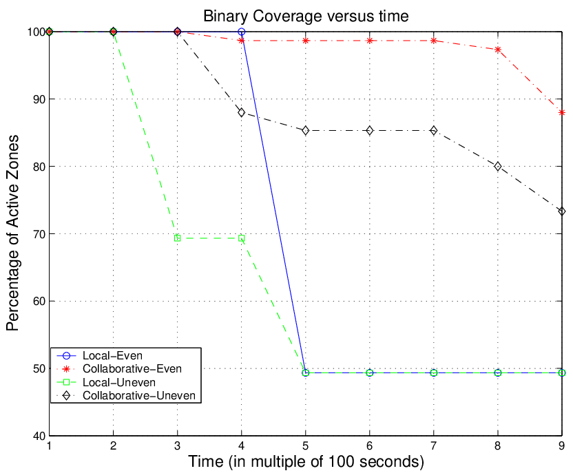
Figure 5 shows the Binary Coverage as a function of time. One can see that CBCS has a higher percentage of active zones compared to LS for both data generation models.

Similar trends are seen when considering Manifold Coverage (Figure 6). Each line represents the percentage of zones with some specific coverage level: for example, the line “quarter” represents the percentage of zones where at least 25% of the sensors have storage space left. One can clearly see that, in the case of LS with even data generation (Figure 6(a)) the percentage of zones with full coverage is 100% at 300 seconds, whereas with uneven data generation it reduces to less than 50% within 300 seconds. In CBCS, at the same times, the coverage is around 96% with the even data generation model and with the uneven data model it is around 77%. Note that, A CH stored more data than individual sensor, therefore if the round time is very long, it might happen that the given CH runs out of storage sooner than a sensor storing its data locally. In LS, the percentage of dead zones (zones with all sensors out of storage space) rises in two waves for the uneven data model, reaching up to 30% within 300 seconds and 50% in 500 seconds However, with CBCS, with the uneven data model, the percentage of dead zones rises slowly and is below 30% even at the end of the simulation. In general, from these figures, one can see that the manifold coverage changes are abrupt for local buffering. In contrast, collaborative storage provide smooth degradation of coverage. Moreover, the average coverage is higher for collaborative storage due to the data aggregation and load balancing ability. by transferring data from high activity zones to low activity zones.

One limitation of the aggregation model we have used so far is that the required storage size under collaboration grows in direct proportion to the number of sensors in the cluster; that is, the storage consumed in a round is $\alpha N\cdot D$, where $\alpha$ is the aggregation ratio, $N$ is the number of sensors and $D$ is the data sample size. Since the available storage ($N\cdot S$, where $S$ is the available storage per sensor) is also a function of the number of sensors, storage is consumed at a rate ($frac{\alpha D}{S}$) which is independent of the number of sensors present in the zone, assuming perfect load balancing. For most applications, this will not be the case: the aggregated data necessary to describe the phenomenon in the zone does not grow strictly proportionately to the number of sensors and we expect storage lifetime to be longer in dense areas than in sparse ones.

To highlight the above effect, we consider the case of a biased deployment where sensors are deployed randomly but with non-uniform density. In addition to the aggregation model considered so far, we consider a case where the CH upon receiving packets from its $N$ members, just needs to store 1 packet. As an example if the aggregation function is to store the average value of the $N$ samples (e.g. average temperature reading). Clearly, in the second case, the size of the aggregated data is independent of network density. We now study how these applications with different aggregation functions perform on top of a biased deployment. To model biased deployment, we consider 4 zones with 5,4,3,2 sensors respectively. In these simulations, the round time was set to 10 seconds (CH selection happens every 10 seconds).

In Figure 7, the X-axis shows time (in multiple of 10 seconds), whereas the Y-axis shows the percentage of coverage sensors within a given zone. As described earlier we considered 4 zones for this study and each line in the Figure 7 represents a particular zone. For example line Z-5 stands for a zone with 5 sensors in it and Z-2 denotes the zone with 2 sensors in it and so on. As shown in Figure 7(a), when the aggregation ratio is a constant (0.5), all the zones provide coverage for almost same duration. However, in the second case, as shown if Figure 7(b), coverage is directly proportional to the network density, higher the density, longer the coverage.

The sensor network coverage from a storage management perspective depends on the event generate rate, the aggregation properties as well as the available storage. If the aggregated data size is independent of the number of sensors (or grows slowly with it), the density of the zone correlates with the availability of storage resources. Thus, both the availability of storage resources as well as the consumption of them may vary within a sensor network. This argues for the need of load-balancing across zones to provide long network lifetime and effective coverage. This is a topic of future research.

References

- [1] G. Asada, M. Dong, T. Lin, F. Newberg, G. Pottie, and W. Kaiser. Wireless integrated network sensors: Low power systems on a chip. In European Solid State Circuits Conference, Oct. 1998.
- [2] N. Bulusu, J. Heidemann, and D. Estrin. GPS-less low cost outdoor localization for very small devices. IEEE Personal Communications Magazine, Oct. 2000.
- [3] A. Chandrakasan, A. Amirtharajah, S. Cho, J. Goodman, G. Konduri, J. Kulik, W. Rabiner, and A. Wang. Design considerations for distributed microsensor systems. In Proc. of the IEEE 1999 Custom Integrated Circuits Conference (CICC’99), May 1999.
- [4] D. Ganesan, B. Greenstein, D. Perelyubskiy, D. Estrin, and J. Heidemann. An evaluation of multi-resolution storage for sensor networks. In Proceedings of the ACM SenSys Conference, Los Angeles, California, USA, November 2003. ACM.
- [5] W. Heinzelman. Application-Specific Protocol Architectures for Wireless Networks. PhD thesis, Massachusetts Institute of Technology, 2000.
- [6] J. Hill, R. Szewczyk, A. Woo, S. Hollar, D. Culler, and K. Pister. System architecture directions for network sensors. In Proc. of ASPLOS 2000, Nov. 2000.
- [7] C. Intanagonwiwat, D. Estrin, R. Govindan, and J. Heidemann. Impact of network density on data aggregation in wireless sensor networks. Technical Report TR-01-750, Univ. of Southern California, Nov. 2001.
- [8] P. Juang, H. Oki, Y. Wang, M. Martonosi, L. S. Peh, and D. Rubenstein. Energy-efficient computing for wildlife tracking: design tradeoffs and early experiences with zebranet. In In Prof. of ASPLOS 2002. ACM Press, 2002.
- [9] Crossbow – smart sensors in silicon (crossbow website), 2003. Commercial product based on Berkeley MICAs http://www.xbow.com).
- [10] Network Simulator. http://isi.edu/nsnam/ns.
- [11] S. Ratnasamy, D. Estrin, R. Govindan, B. Karp, S. Shenker, L. Yin, and F. Yu. Data-centric storage in sensornets. In Proceedings of the First ACM SIGCOMM Workshop on Hot Topics in Networks, Oct. 2002.
- [12] A remote ecological micro-sensor network, 2000. (http://www.botany.hawaii.edu/pods/overview.htm).
- [13] SimpleTech flash memory card datasheet. http://www.simpletech.com/products/consumer/data_sheets/R187.pdf.
- [14] S. Tilak, N. Abu-Ghazaleh, and W. Heinzleman. Storage management issues for sensor networks. In Student Posters (ICNP 2003), movember 2003.
- [15] Y. Xu, J. Heidemann, and D. Estrin. Geography-informed energy conservation for ad hoc routing. In Proceedings of the 7th annual international conference on Mobile computing and networking. ACM Press, 2001.
- [16] Y. Yao and J. Gehrke. The cougar approach to in-network query processing in sensor networks. SIGMOD Record, 31(3), Sept. 2002.