An algorithm for two-dimensional mesh generation based on the pinwheel tilingThanks: Supported in part by NSF Grants CMS-0239068 and CCF-0085969
Abstract
We propose a new two-dimensional meshing algorithm called PINW able to generate meshes that accurately approximate the distance between any two domain points by paths composed only of cell edges. This technique is based on an extension of pinwheel tilings proposed by Radin and Conway. We prove that the algorithm produces triangles of bounded aspect ratio. This kind of mesh would be useful in cohesive interface finite element modeling when the crack propagation path is an outcome of a simulation process.
1 Introduction
One of the most widely used techniques to simulate fracture is cohesive interface finite element modeling. In this kind of model, the area or volume under consideration is subdivided into bulk elements, which are typically triangles or quadrilaterals in 2D and tetrahedra or hexahedra in 3D. Next, interfacial elements, which are edge elements in 2D or surface elements in 3D, are placed between some or all pairs of adjacent bulk elements. The cohesive model prescribes a relationship relating traction to relative displacement on the interfacial elements. There is an abundance of literature that deals with the nature of this relationship, e.g., see [5] and the references therein. A widely accepted modeling assumption is that the total energy to create the crack is proportional to its surface area (or length in 2D). In fact, the critical energy release rate per unit surface area or length of crack is often a parameter of the cohesive model.
In a finite element model, the energy release rate is associated with surface area or length of interfacial elements composing the crack being modeled. If the discrepancy between the “true” crack path (i.e., the path the crack would follow if it were not for the finite element constraint that the crack path must lie on predetermined interfacial elements) and the path of the simulated crack is large for certain paths, then nonphysical preferred crack directions can exist. In other words, the results of the simulation would depend upon how well the boundaries of the mesh cells are aligned along the true crack path. In this paper, we propose a meshing technique that approximates the true path with the path along mesh boundaries with high accuracy even though the true path is unknown to the mesh generation algorithm. In particular, the approximation has the property that for any crack path, the simulated and true crack path lengths converge to each other upon refining the mesh, which is a property not possessed by other simpler families of meshes. We call this algorithm the PINW mesh generator because it is based on an extension of the 1:2 pinwheel tiling described in the next section.
In Section 3 we define “deviation ratio” and consider a simple experiment to test the properties of the 1:2 pinwheel mesh. The 1:2 pinwheel tiling seems to be too restricted to be useful for a general-purpose algorithm, so we explain how to generalize it to arbitrary triangles in Section 4. This generalization is the basis for our meshing algorithm PINW. In Section 5 we prove that our generalization still has the isoperimetric property. Then in Section 6 we describe the algorithm. The main new ingredient introduced in that section is a procedure to convert a tiling to a mesh. The aspect ratio of the resulting mesh is analyzed in Section 7.
The aspect ratio of the mesh is important for the cohesive fracture application because the bulk elements (e.g., triangles in 2D) are used to model a continuum mechanical theory such as linear elasticity. It is well-known (see, e.g., Theorem 4.4.4 of [2], in which aspect ratio is called “chunkiness”) that poorly shaped elements can lead to substantial errors in the elasticity solution.
2 Pinwheel tilings
In this section, we provide a brief introduction to the properties of pinwheel tilings. Tilings are a covering of the euclidean 2-space starting with a finite number of shapes called prototiles. The tilings are constructed by translated and rotated copies of the prototiles that intersect each other only along the boundaries. The tilings were proposed to model crystallographic structures in the physics community.
The pinwheel tilings [6] are classified as aperiodic tilings. In this is equivalent to saying that no translation of the tiling leaves it invariant. The basic pinwheel tiling as developed by Radin and Conway has a hierarchical structure and is constructed by successive operations of subdivisions and expansions.
Consider a right triangle with legs of length and referred to as the short and medium sides. The hypotenuse is thus of length and will be called the long edge. The vertices will be named similarly, that is, the small, medium and long vertices are opposite the corresponding sides. For brevity, we will call a right triangle with the ratio of its short to medium edge equal to as a “ right triangle” and the tiling formed by its copies as a “ tiling.” This single tile is subdivided into five triangles that are all congruent to each other as shown in Figure 1.
If one were to dilate the subdivision in Figure 1 by a factor of and then rotate and translate the resulting figure so that the dilated copy of ended up coincident with the original tile , then a larger subset of would now be tiled. The above subdivision scheme is then applied to each of the five copies of , and then another dilation followed by rotation and translation is carried out. Continuing this process infinitely would lead to a tiling of the plane. Thus, in the case of the standard pinwheel tilings, and (where denotes the reflection of about the x-axis) form the set of fixed prototiles and the tiling uses translations and rotations of this set.
For our purposes however, we will concentrate just on the subdivision step and omit the dilation, translation and rotation steps, leading to the “subdivision” pinwheel tiling in which the cell diameter tends to zero and the area of the plane covered by the mesh does not expand from step to step. This is because we are interested in generating a mesh with varying amounts of refinement for a fixed region rather than a mesh that ultimately covers . In the subdivision pinwheel tiling, one starts with a fixed triangle and then repeatedly subdivides first the initial triangle and then each subtriangle into five congruent subtriangles using the above rule.
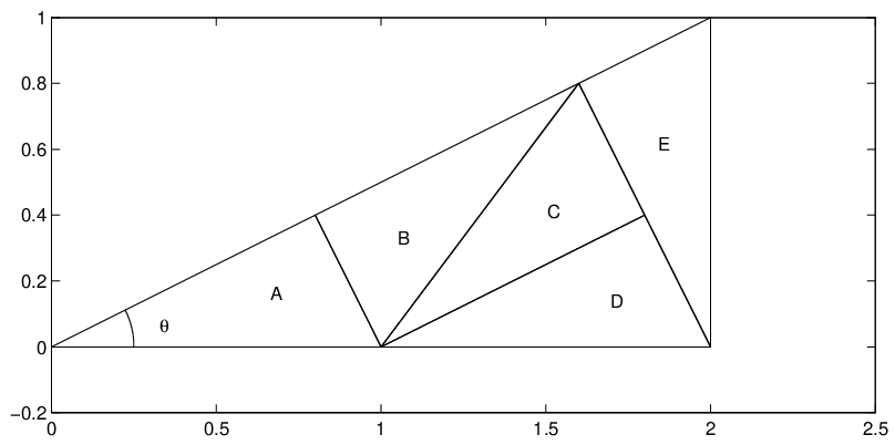
One can enumerate the rotation angles of the child triangles with respect to and as , , , , where is rotation by in the counterclockwise direction. For the standard right triangle, and in this case is irrational. The significance of this is as follows. As the number of subdivisions goes to infinity, so do the distinct orientations of the triangles. For example, suppose we keep track of the orientation of all triangles of type with respect to the parent triangle in the subdivisions. As can be seen in Figure 1, the angle made by a triangle of type with respect to the parent in the th subdivision is . Since is irrational, will represent a different angle for each .
This presence of an infinite number of orientations leads to a special property known as the isoperimetric property [7]. For a tiling of , isoperimetry means that given an , there exists an such that for any two points and on the boundaries of the triangles with , the shortest path from to that uses only tile edges has length at most . Here denotes the Euclidean distance from to , which will also be denoted as .
There is an analogous property for the subdivision pinwheel tiling. In this case, let , be two points on the boundary of the initial triangle. Then for every , there exists an such that after recursive subdivisions of the initial triangle, the shortest path from to using only triangle edges is at most . This theorem can be generalized so that and do not have to be on the boundary of the initial triangle but may be any two distinct points.
The isoperimetric property is the reason that pinwheel tilings are attractive for cohesive interface modeling. Consider a finite region tiled with an infinite sequence of pinwheel tilings in which the triangles in all have side lengths , , , and as . Then for an arbitrary straight segment of length connecting to , and for an arbitrary , there exists an such that in each of the tilings , there is a path from to using only mesh edges (except for initial and ending segments to connect and to the boundaries of the triangles that contain them) such that the length of the path is . We will give a proof of this result in a more general setting in Section 5.
Since the above result holds for an arbitrary line segment, it also holds for any piecewise smooth curve or network of such curves. The reason is that a network of piecewise smooth curves can be approximated arbitrarily accurately with a network of line segments. Then each of the line segments can be approximated arbitrarily accurately with paths of the pinwheel tiling.
Thus, when used for cohesive fracture, the pinwheel tiling has the property that all possible crack paths are approximated as accurately as desired (in terms of their length) by paths that use only mesh edges, as the mesh diameter tends to zero. As we shall see in the next section, more common mesh generation techniques do not have this property.
3 A computational experiment
In this section we carry out some simple experiments to quantify the isoperimetric property of the 1:2 tiling. Since our interest here is in meshes, we first explain how to convert the 1:2 pinwheel tiling to a mesh. It is apparent from Figure 1 that the pinwheel tiling is almost a triangulation except for the hanging node bisecting the medium side of triangle . We define a hanging node of a planar subdivision into triangles to be a point that is a vertex of one triangle but lies on the strict relative interior of an edge of another triangle.
It is fairly simple to make the pinwheel tiling a mesh [6]: we divide every triangle into two by joining its medium vertex to the midpoint of its medium edge. In fact, it is not necessary to split all the triangles, and in our example we have obtained a mesh by splitting a certain subset of the tiles. This splitting is done only on the finest level of the pinwheel subdivision.
Our computational experiment is as follows. Starting from a rectangle, we divide it into two triangles and then apply the pinwheel subdivision times to each of the triangles. Thus, the final tiling has triangles. The resulting tiling of the original rectangle is then converted to a mesh using the technique in the last paragraph.
Given a tiling of a domain , let be the 1-skeleton of , that is, the union of all edges of all triangles, and let be the set of all vertices of . Let be a positive parameter chosen small enough so that contains a disk of diameter . We propose to evaluate isoperimetric quality of the triangulation with the following quantity, which we refer to as the -path deviation ratio:
Here, means shortest distance among paths restricted to . The notation means the geodesic distance from to , i.e., the shortest path among paths lying in . Thus, this quantity measures the maximum ratio between the paths in the mesh versus geodesic paths. Clearly for any mesh of any polygon, . The pinwheel mesh of the 1:2 rectangle has the property that for any , as where is the pinwheel tiling of the rectangle after levels of refinement.
Our experiment is to evaluate for . The results are depicted in Table 1. The worst-case shortest path is shown in Figure 2.
| 1 | 1.3416 |
|---|---|
| 2 | 1.1948 |
| 3 | 1.1843 |
| 4 | 1.1264 |
| 5 | 1.0831 |

In contrast, consider the meshes in Figure 3. The deviation ratios of these meshes have lower bounds greater than 1 irrespective of the number of subdivisions. In particular, the lower bound is for the mesh in Figure 3. For the mesh that was used by Xu and Needleman [10] (one of the first papers on cohesive finite element modeling), which is shown in Figure 3 and is sometimes called a “cross-triangle quadrilateral” mesh, the worst case deviation ratio can be shown to be approximately equal to in the limit as the mesh cell size tends to 0.
4 Generalization of Pinwheel Tilings
The pinwheel tiling discussed up to now was extended to a tiling with an arbitrary right triangle and its reflection as a prototiles by Sadun [8]. The small angle of the prototile determines the finiteness of the orientations and sizes of the tiles in the tilings that are discussed in [8]. We now describe our approach to extend the pinwheel subdivision to arbitrary (non-right) triangles.
First we propose a way of subdividing a general triangle and show that any number of subdivisions would produce triangles similar to a finite set of prototiles. Consider the triangle shown in Fig. 4. We denote the vertices by , and in clockwise order and the included angles at these vertices by , and respectively. Assume also . First, draw the segment such that is a point on and measured counterclockwise from . From draw such that is on and measured clockwise from . From draw and such that is on and is on and clockwise from and counterclockwise from . Thus, we have a subdivision of a general into five triangles of which , and are similar to the parent and the remaining two and are similar to each other but not to the parent. Note that we required to make this construction but we did not require any ordering on .

Theorem 1.
The above procedure for subdivision produces triangles with angles belonging to the set or to the set .
Proof.
This is obvious by simply checking all the angles in Figure 4 and using the fact that angles of a triangle sum to . ∎
Theorem 2.
If the above subdivision procedure is used recursively on the subtriangles, then any triangle produced has angles either from or .
Proof.
One checks that if we define , , then . ∎
For the rest of this paper, we say that a triangle with angles (listed in this order) is conjugate to a triangle with angles . The point of Theorem 2 is that conjugacy is a symmetric relationship. We remark that if the original triangle is a right triangle, i.e., , then this triangle is similar to its conjugate. This is the case considered by [8].
These two theorems imply a procedure for subdividing any initial triangle with angles , , . Assume . Apply the first subdivision rule to get five smaller triangles. Then, for the three similar to , reapply the same rule recursively. For the two conjugates, apply the other rule. For the conjugate triangles, we do not necessarily have the order , but we do not need that order. We need only the inequality , which must be true since .
This procedure runs into a difficulty when (i.e., the initial triangle is close to equilateral) because in this case the conjugate triangle will have a bad aspect ratio. We get around this problem as follows. If , then we first subdivide the initial triangle into three about its in-center, that is, we join the in-center to the vertices of the original triangle and form three subtriangles. We use a cutoff in our algorithm: if is less than the cutoff, then the preliminary tripartition is carried out. The cutoff for is chosen to optimize the smallest angle. In other words, a parent is divided about the in-center if the smallest angle prior to division is smaller than after the division. Here smallest angle happens to be the minimum of the angles in the two sets and for a given set of angles and can be shown to be rad. Thus, we take the cutoff to be 0.4 rad.
5 Isoperimetric property
This section is devoted to showing the result that the generalization of the pinwheel tiling introduced in the previous section obeys an isoperimetric inequality. The analysis and proof technique in this section closely follow the proof from [7]. The following is the key lemma in the proof of isoperimetry.
Lemma 1.
Let triangle be as above. Assume is an irrational number, where is the angle of at . Let and be arbitrary. Then there is a refinement of following the above rules that contains a triangle edge such that the angle between and the -axis lies in the interval .
Furthermore, the length of is at least , where are the angles of , is as above, is a fixed positive-valued function, and is the longest side-length of .
Proof.
Observe that Triangle III in the above subdivision is similar to the initial triangle but is rotated by angle . Call this triangle . If this triangle is subdivided by the same rule again, there will be another smaller copy of , say , rotated by etc. The infinite sequence taken mod is dense in the interval by the assumption that is irrational. Therefore, for some sufficiently fine mesh, there is an edge of triangle in the interval .
For the second part of the lemma, observe that for any there is an such that every point in is distance (mod ) at most from at least one point in the set . Therefore, one of described in the last paragraph will have the desired edge . The longest side-length of is ; the longest side-length of is , where is some universal function (not depending on anything other than ) derived from our construction. By similarity, the longest edge of has length . Thus, if we define , where is the ratio of the shortest to longest side length of , then the length of is at least . This proves the second part of the lemma is also satisfied. ∎
For the first main theorem of this section, we need one more definition. We say that a generalized tiling of a triangle refines another generalized tiling of provided that for each tile of , either appears in or a subdivision of appears in . This definition implies that and . The first main theorem for this section is as follows.
Theorem 3.
Let be a triangle with angles such that and is irrational. Let be an infinite sequence of generalized tilings of generated by the rules above. For each , let be the maximum tile diameter in . We assume the sequence of tilings has the following two properties: (a) refines , and (b) as . Let be any two points on the boundary of . Then
In other words, every straight-line path connecting two points on the boundary of is approximated with arbitrary accuracy by a path of edges of the tiling.
Proof.
In order to prove this theorem, we require a simultaneous analysis of tilings of a conjugate triangle. Therefore, let us change notation so that the original triangle is , its conjugate is , and there are two sequences of tilings with the above two properties, namely, , which are tilings of , and , which are tilings of .
Without loss of generality, let us further assume that for is simply , and that each subsequent is obtained from by splitting exactly one tile (so that has exact tiles). This assumption is without loss of generality because we can take our original given sequence , etc., and insert all intermediate tilings (i.e., if the original was obtained from via subdivision operations, then we can insert intermediate tilings in the sequence). If we prove that the limiting property holds for the augmented sequence, then it certainly also holds for the original sequence.
We make the following preliminary observation about generalized pinwheel tilings. If is any tiling of for or obtained from the above generalized subdivision rules, then there exists an such that refines .
We use the following additional definitions and notation to prove the theorem.
- •
Let denote the boundary of , . Thus and are each unions of three segments.
- •
Define , for
- •
For any , let denote .
- •
For , let , . If we took the maximum of this quantity over choices of , we would arrive at a quantity analogous to the “deviation ratio” introduced above in Section 3. Clearly for all . If , then define to be 1.
- •
Let . Note that is a nonincreasing function of (because every edge of is covered by edges of for all ), so this is also the limit of the sequence.
- •
Let . Clearly for all . For the same reason as above, is also the limit of the sequence.
The main theorem now reduces to showing that for all . Our proof technique requires us to claim more strongly that for all and for and .
- •
Let be the length of the shortest edge of for . Let be the length of the shortest edge among the five triangles that result from one application of the splitting rule to , and let .
- •
Let denote points such that and such that . Note that is a compact set under the norm specified above.
The reason for introducing is that is continuous on as the following argument shows. Observe that for , . The function is continuous on all of because it is a metric. The denominator is also continuous and bounded away from 0 on , hence is continuous on this set. (Once the theorem is proved, then it is established that is continuous on all of , but this is not so easy to prove at this stage of the argument.)
The following lemma shows that it suffices to analyze rather than all of .
Lemma 2.
For ,
Proof.
Choose an arbitrary . This proof will show that
Taking the supremum on the left will prove the result. If then the result is immediate since that value appears in one of the two terms in the right-hand side. So assume for the rest of the proof that . If lie on the same side of , then the left-hand side is 1 because for all in this case since the boundaries of are covered by the edges of for each . Since the right-hand side is greater than or equal to 1, the result follows immediately.
The last case is that are on distinct sides (and in particular, are not vertices of ). In this case they must be less than distance of the same vertex by definition of . For the rest of the proof of this lemma, consider only the case since the case is similar.
First, suppose that are both within distance of , the vertex whose angle is . Without loss of generality, lies on and lies on . Consider the sequence of tiles such that is the tile from that contains vertex . Each of these tiles is similar to . The diameter of the ’s tends to 0 as by assumption. Thus, there is a such that contains both and but fails to contain one or both of or . Let be the length of the shortest side of . We claim that either or . The reason is that if both and then would both lie on the boundaries of since the side lengths of are all at least by definition of . This would contradict the choice of .
As mentioned above, is similar to , and the constant of proportionality is . Note that could be either a dilation of with no reflection or a dilation of with a reflection. Assume the former case since the latter is similar. There exist and lying on sides , of whose positions with respect to , are proportional to the positions of with respect to the two sides of . Since either or and the scaling factor between and is , this means that at least one of , is distance from greater than or equal to . Hence . For an arbitrary , consider the tiling of that is obtained by shrinking by a factor of and translating it so that it lies on top of . The shortest path between and in this tiling is by scaling. Also, there is an such that the portion of lying in is strictly a refinement of by the observation made at the beginning of the proof. The distance between and in this tiling is , and since refines , . Note that by similarity, so the previous inequality implies . Take the infimum over all of both sides to conclude that , thus establishing the lemma in this case.
In case that are both within distance from vertex whose angle is , the lemma follows by the same argument since the triangles containing in all subdivisions of are similar to .
The last case is that are both within distance of vertex whose angle is . Say, e.g., that lies on and on . In this case, the argument is slightly more complicated since there are two triangles containing in the next level of subdivision. Let be the segment that is the common boundary to the two triangles of the next level of subdivision that meet vertex . (Refer to Fig. 4.) Let be the point where segment crosses edge . Then the argument above shows that the infimum over of the distance between and using edges from is less than or equal to , where . Similarly, the infimum over of the distance between and using edges from is less than or equal to , where . Therefore, so the result follows. ∎
Finally, we conclude the proof of the main theorem by showing that for . To this end, choose (either 1 or 2) so that . Without loss of generality, say is chosen.
Since is a compact set and is continuous on this set, there exists a in that maximizes . If lie on the same side of , then so the proof is finished. Else let the corresponding pair of points where the supremum is achieved be and be the line segment joining them. Assume (for a contradiction) that .
Choose large enough so that there exists a tile in such that has positive length and is contained in the middle third . Let the longest edge of be . For reasons to be explained below, we also choose large enough so that
| (1) |
where is the function defined by Lemma 1. Continue splitting until we reach split number so that within , there exists a tile in lying inside in that has an edge making an angle with , with . This is possible by Lemma 1. See Figure 5. Let be the length of this edge. By the second part of the lemma, we may assume , where .

Let be the endpoints of this edge with being the vertex near and near . Observe that , and make up a three-segment path from to . The length of this path is , where and (We have already defined .) Let , , and be the lengths of the projections of , , respectively onto . Because lies within while crosses through , the distance from to is at most , hence
hence
| (2) |
(The factor of 3 arises because as assumed earlier.) Similarly,
| (3) |
Next, because where is the angle between and , we have . Therefore,
| (4) |
Next, note that thanks to the existence of the three-edge path . The reasoning is as follows. From to there is a straight-line path of length . This path cuts through a finite list of triangles, say triangles, within the tiling , since and both lie on triangle edges of this tiling. Let the individual segments within these triangles be of length . By construction, these quantities sum to . Then by further refinement, we can find paths within the tiling with lengths less than or arbitrarily close to , , etc. since is the factor that is the maximum amount longer that an edge path in refinements of either or can be versus the straight-line path. So the infimum of the lengths of these paths added up is at most . The same reasoning accounts for the term . Finally, the edge is length and is already in the tiling.
The preceding theorem has the drawback that it pertains only to paths starting and ending on the boundary of the root triangle. For isoperimetry, we would like to generalize the result to paths with arbitrary interior and . Since the nodes of the pinwheel tiling are dense in the interior (in the limit as the mesh size is refined), the following theorem provides a suitable generalization and will be taken as our definition of the isoperimetric property.
Theorem 4.
Let be a sequence of generalized pinwheel tilings of (satisfying and is irrational as in the previous theorem) such that the maximum cell diameter tends to zero and such that refines for all . Let be any pair of distinct points lying on for some . Then
Proof.
Consider the segment lying in . Let be given. Make a list of tiles in traversed by this segment. Since crosses , define to be . Observe that both lie on the boundary of . By the preceding theorem, after a sufficient number of further subdivisions (say ), there exists a path in between and of length . This choice of depends on , so take the maximum such value of (maximum over all ). Then there is a path in from to of length at most
i.e., at most . ∎
6 Meshing an arbitrary region
In this section we present our algorithm PINW to mesh a region with arbitrary polygonal boundary. A summary of PINW appears in Figure 6. The steps in this summary are described in more detail in the remainder of this section. The current version of PINW is 1.0 and has been coded in Matlab. An example output from this algorithm is shown in Fig. 7.
Algorithm PINW 1.0 1. Generate a mesh for with bounded aspect ratio using Triangle. 2. Split triangles too close to equilateral at their in-centers. 3. Split triangles whose smallest angle is a rational multiple of at a point near the in-center. 4. Let the set of triangles obtained after steps 1–3 be called . 5. Initialize a heap containing triangles that need splitting. The triangles are ordered so that the one whose minimum altitude is maximum is at the top of the heap. Initially the heap contains all triangles from . 6. Repeatedly remove a triangle from the heap and split it into five, until the size of the top element of the heap is sufficiently small according to the user’s specification. 7. Let be the set of tiles including those in and all their descendants obtained by subdivision. Let be the set of leaf tiles. 8. Loop over all tiles in starting from the coarsest to determine the value of for each edge of any tile. 9. For each big edge (i.e., each edge in the image of the “big” operator), select one side as moving and the other as staying. Sort the list of nodes lying on the staying side of each such edge. 10. Loop over tiles in starting from the coarsest excluding . For each such tile and for each of its vertices as labeled in Figure 4, let be the maximal big edge containing the particular vertex. If this vertex , or is on the moving side of and is very close to a vertex on the staying side, then displace it to coincide with and apply the induced affine transformation to subtriangles of . 11. Apply Delaunay triangulation to each distorted, subdivided leaf tile. (The distortion of the leaf tiles is due to the affine transformations in the previous step. The subdivision of the edges is due to the presence of hanging nodes.) The collection of triangles output from this step is a simplicial mesh of .

We first start with a coarse triangulation of the domain. We use the Triangle package [9] developed by J. Shewchuk, which uses Delaunay triangulation. The triangles produced have bounded aspect ratio. The second preliminary step, as mentioned in Section 4, locates triangles too close to equilateral and splits them at their in-center.
A third preliminary step is to identify and split triangles whose smallest angle is a rational multiple of . (As noted above, the proof of isoperimetry requires that be irrational.) In principle, this test could be conducted exactly using number-theoretic methods since the coordinates of the vertices of each triangle, being floating-points numbers, are rational numbers and can be treated with integer algorithms by clearing common denominators. Modifying a triangle in which is a rational multiple of is trivial in principle because any small random perturbation of a node of such a triangle will lead to an angle that is not a rational multiple of with probability 1.
In practice, this exact test and solution are both undesirable. For practical use of the algorithm, we would like to avoid the case when is close to a rational multiple of of the form where is a small integer. The reason is that the presence of such a triangle in which is irrational but is close to implies that, although the isoperimetric property is asymptotically valid, the available angles will be badly distributed (clustered around multiples of ) for modest levels of refinement.
Therefore, a more practical heuristic is to check each smallest angle against a finite list of the form , where range over a pre-selected set of small integers. If a triangle’s smallest angle comes too close to a member of this list, then the triangle is either split into three using a point near its in-center or is perturbed. (The exact in-center obviously should not be used since this would replace each angle by half its previous value, and hence still close to a rational multiple of .) This step has not been implemented in the current version of our code PINW 1.0 because we are still seeking the best practical heuristic. (Indeed, in Figure 7, one coarse triangle is close to a 45-degree right triangle, and hence one part of the subdivision exhibits a shortage of possible directions.)
Let be the list of triangles that are produced by these preliminary steps. Thus, the triangles in form a simplicial triangulation of the input set . We call these triangles the root tiles. The generalized pinwheel subdivision is then performed on the the root tiles to obtain a refined tiling. The procedure to refine the mesh used in PINW 1.0 is based on a simple heap [1]. The heap is initialized with all triangles in , which are ordered in the heap according to length of the minimum altitude. The main loop for the subdivision is to remove the top member of the heap (i.e., the unsubdivided tile with the largest value of minimum altitude) and replace it with its five children. The procedure terminates when the top triangle in the heap is smaller than the user-specified mesh size requirement.
Note that during the subdivision procedure, the angles in Figure 4 are assigned to smallest, middle and largest angles respectively for tiles similar to root tiles. For the conjugate tiles, angles are assigned according to the conjugacy relationship. In other words, if the angles of the root tile are in that order, then the angles in the conjugate tile are assigned in the order , , and . This ensures that the conjugate of the conjugate is again similar to the root tile.
From this description, it is apparent that PINW 1.0 supports a single global user-specified mesh size requirement. For many applications of mesh generation, it is useful to have a finer mesh in one part of the domain versus another. This can also be implemented in the framework of generalized pinwheel subdivision but is not available in PINW 1.0. In addition, several aspects of our analysis that follows below would have to be generalized to cover graded meshes.
Once the subdivision procedure is complete, the resulting tiling must be converted to a simplicial mesh. For the 1:2 pinwheel triangulation, this step is quite straightforward as mentioned in Section 3. In the generalized case, however, it is much more complicated and involves several steps that we shall now describe.
Let be the list of all tiles in the hierarchy: it includes the tiles in and all their descendants from the subdivision procedure. The tiles in naturally have a forest structure associated with them in which the forest roots are root tiles. Let leaf tile denote a triangle in that is not further subdivided during the generalized pinwheel subdivision phase. Let be the set of leaf tiles.
The first step in converting the tiling to a mesh is to identify for each edge of each tile the edge that we denote . This is defined to be the edge of a triangle higher up in the subdivision hierarchy (i.e., is derived from via a sequence of zero or more subdivision operations) such that , and such that is maximal with this property (i.e., there is no other ancestor of with an edge that strictly contains ).
For each triangle in , . For some other tile with an edge , it is a straightforward matter based on a checking a finite number of cases whether or . In the latter case, can be determined from the immediate parent of (assuming is already tabulated for the the parent’s edges). Thus, it is possible to determine for each edge of each tile in with a constant number of operations per tile.
Next, for each “big” edge (that is, an edge such that ), identify a moving and staying side. This choice can be quite arbitrary, except for two stipulations. An edge adjacent on the exterior boundary of should have its inside labeled staying (i.e., no tiles lie on its moving side). An edge in correspondence with in Figure 4 (every big edge generated during the subdivision procedure is in correspondence with either , , or ) should have the side facing vertex labeled as moving. We now identify all the nodes on the staying side of and sort them in order of occurrence on the edge. This sorted list is saved for the next phase of the algorithm.
In the next phase, we loop over triangles in starting from the coarsest and perform collapse-node operations on each. Let be a tile in . Let the four vertices of introduced when it is subdivided be labeled as in Figure 4. We perform no operation for since it is on the staying side of edge . The maximal big edge containing is ; call this . The maximal big edge containing and is ; call this and also call it . Let be one of . We check whether is on the moving side of . If it is on the staying side, then no further operation is performed. If it is on the moving side, then we find the vertex taken from the staying side of that is closest to . This can be found efficiently using binary search on the precomputed sorted lists. If , we collapse nodes and by displacing to . Here is a tolerance discussed more below.
This displacement induces uniquely determined affine transformations on triangles contained in as follows. If is the vertex labeled in Figure 4, then there is a unique affine transformation on that leaves and fixed and moves to . A second affine transformation of leaves and fixed and moves to . If is the vertex labeled , then there are unique affine transformations determined for and . Finally, if is the vertex labeled , then there are transformations for each of , and . The algorithm applies all the relevant affine transformations caused by motion of the node. Note that the affine transformations agree on the boundaries between these triangles, so there is no consistency issue regarding which transformation to apply. These transformations move the triangle, including every node at deeper levels of the hierarchy contained in it. This concludes the description of the collapse-node operation. See Figure 8 for an illustration of this operation.
Note that a single tolerance is used to determine motion. The theoretical value for is given by below. We will verify later that this value of is sufficiently small so that two important properties hold:
- Property 1 of :
-
If a vertex is the target of a collapse-node move, then it should be uniquely determined, i.e., there should not be two vertices and on the staying side of that are both within distance of .
- Property 2 of :
-
No two vertices on the moving side of for any should be collapsed to the same node on the staying side.
In a future extension of PINW to handle graded meshes, presumably the value of would not be a single global value.
The affine transformations described above have the property that all of the segments illustrated in Figure 4 remain straight (collinear) segments after the transformation. It is apparent that each collapse-node operation could cause many nodes to move. We will say that the one node that is displaced to match is directly displaced. The nodes moved by virtue of an affine transformation induced by moving are said to be indirectly displaced.
A collapse-node operation, once executed, cannot be undone by future collapse-node operations. The reason is that is never moved again. It is never moved again directly since it can be moved directly only when the tile that created it is processed. It can also never be moved again indirectly since there is no tile in lower levels of the hierarchy that contains it except as a corner vertex, and corner vertices of a triangle are not moved when is processed. Similarly, can never be moved again. The reason is that is never moved directly (since it is on the staying side of its big edge). Any transformation that might move indirectly takes place at a level of the hierarchy higher than the level of .
We carry out all available collapse-node operations for all triangles in the order described. Once all collapse-node operations are complete, we are left with the collection of distorted leaf tiles, each of which may have one or more hanging nodes. These hanging nodes are collinear with the endpoints of the edges on which they hang because, as noted above, we do not disturb any collinearity relationships with collapse-node operations. The hanging nodes are all at least apart from the corners and from each other.
For each of these distorted tiles, we compute its Delaunay triangulation (including the hanging nodes). The collection of all of these Delaunay triangles forms a simplicial mesh that is the final output of PINW.
The running time of PINW is analyzed as follows. Let be the number of leaf tiles. Then the total number of tiles is , as is the total number of vertices and edges. The heap insertions and deletions require total operations. Sorting all the lists associated with big edges requires operations. Looking up a vertex in a sorted list requires operations for binary search, hence all of the lookups to see if a node should be collapsed require operations.
The recursive application of affine transformations requires operations since each vertex is transformed at most times, where is the maximum depth of the forest associated with . We claim . It follows from Lemmas 5 and 6 in the next section that the minimum altitude of a triangle at depth lies between and , where are lower and upper bounds on the minimum altitudes among root tiles, is an absolute constant and is a scalar depending on the worst aspect ratio among root tiles. This means that a leaf tile can be at most a factor (asymptotically) deeper in the forest than any other leaf tile. Thus, all leaves have depth .
Finally, the Delaunay triangulation operations in the last step of the algorithm also require operations total. Overall, we see that PINW requires operations.
7 Analysis of aspect ratio
In this section we analyze the aspect ratios of triangles produced by PINW, showing that they are bounded above by a number that depends only on the sharpest angle in the original polygon . Before this analysis, we first explain how to select the parameter described in the last section. The parameter depends on the minimum altitude of leaf tiles as will be apparent from the theory developed here. Let denote the minimum altitude of triangle .
Lemma 3.
Let be a triangle and let . Then can be enclosed between two parallel lines at distance apart. Conversely, if can be enclosed between two parallel lines at distance apart, then .
Proof.
The first part of the lemma is quite trivial: draw a line through the longest side length of and a parallel line through the opposite vertex. These lines are distance apart. The argument for the converse is as follows. Without loss of generality, let the two lines be parallel to the -axis. Let the vertices of be numbered such that is closest to the bottom line (i.e., has minimal -coordinate among the three vertices) and to the top line. By reflecting if necessary, assume also that the -coordinate of is less than or equal to the -coordinate of . Now draw the line , which is a transverse to the two parallel lines. If is below (to the right) this line, then it is easy to see that the entire triangle may be rotated clockwise about until becomes horizontal, and during this whole rotation, all three vertices remain between the lines. On the other hand, if is above (to the left) of the line, then rotate clockwise about until becomes horizontal.
Once has been reoriented so that one of its edges is horizontal, the claim is trivial since the altitude to the horizontal edge is a vertical line segment and hence must have length no more than . ∎
Corollary 1.
If are two triangles such that , then .
Proof.
Draw the two parallel lines for as in the previous theorem; clearly also lies between them. ∎
Lemma 4.
Let be a triangle with vertices . Let be the triangle with vertices . Let be the unique affine transformation that carries to . Let be an arbitrary line segment. Then
| (7) |
where and is the altitude of with respect to .
Proof.
Without loss of generality, assume is 1 and is replaced by . Furthermore, without loss of generality, let be positioned so that its edge is a subsegment of the -axis and lies on the - axis (hence by the previous assumption). With these assumptions, the affine tranformation in the question becomes a linear transformation (i.e., no additive term) since the -axis (and the origin in particular) is invariant. The transformation maps maps to and to . Let , and let be written as so that . Then corresponds to the matrix
The minimum and maximum distortion of a line segment under a linear transformation is governed by the minimum and maximum singular values of the transformation. Thus, the question now hinges on the two singular values of . Notice that may be regarded as a perturbation of the identity matrix, which has two singular values equal to 1. Therefore, by Corollary 8.6.2 of [3], the largest singular value of is at most , and the smallest singular value is at least . These values are attainable by taking and . ∎
Lemma 5.
Consider the generalized pinwheel subdivision illustrated in Figure 4 of a triangle . Assume that and . Then letting be any one of the five subtriangles, we have .
Remark 1. The assumptions are valid for all tiles produced by PINW. For root tiles, we have ordered the angles , and we know because of the preliminary step of splitting near-equilateral triangles. For conjugates of root triangles, say , , and where are the angles of a root tile, we know also and that .
Remark 2. The factor is due to our proof technique and appears to be an overestimate. A search over a fairly dense grid of possible angles satisfying the hypotheses of the theorem indicates that the true bound is closer to .
Proof.
We start by observing that by the law of sines. We know that either or . Furthermore, we know that either or since . Now consider two cases. Case 1 is that . Define , so that , and . On the interval , the sine is increasing. In the subcase that , we have . The last inequality follows because (by assumptions that and ) so . The other subcase is that . Since sine is concave and increasing on the worst case (maximum value) for is when and , so . Thus, . The other case is . This case is handled by the same argument, except using in place of .
Observe that subtriangle V, which is denoted , is similar to except scaled by a factor . This proves .
Next, by similarity, hence . This means . Since is isosceles, and hence and . Next, by the law of sines applied to , . We now take three cases: either , , or . In the first case since the assumption in the lemma is . Also, since and by the assumption for this case, so . This means , with . Next, so (since and sine is increasing on ), so . Now . Thus, . Since is increasing while is decreasing on , the minimum value of this fraction is when , so In the second case, . This means and in particular, so . The last case is , which implies . So the quantity to analyze is . Since the angles in the numerator and denominator are both less than (because ) and , we conclude that .
Thus, in all cases, we conclude that . This means that .
Next, observe that by the law of sines applied to . Again, we take three cases. If (and hence i.e., , i.e., ), then i.e, so . Since all these angles are in , and in this range by the convexity of . The second case is . In this case, so . The last case is . This implies that . The denominator becomes . So we are analyzing , which exceeds 1 since all the angles in question are in . Thus, in all cases, so .
Now we have enough inequalities to analyze where denotes . Observe that this triangle is similar to . Its longest side is either or (but not , since ). If its longest side is , then we see that . (Here we used the fact that , which follows from the hypothesis of this case that plus the similarity of to .) Thus, is similar to but is a factor or less scaled down.
The other case is when the longest side of is . In this case, . The inequality follows from the assumption that and similarity. Thus, is similar to but is scaled down by factor less than . This concludes the analysis of . This same analysis applies to , since is congruent to (because is isosceles).
Next, observe that by the law of sines applied to . Again, we take three cases. If (and hence ), then as above so , so the quantity to analyze is . Using analysis like before, including steps like , we conclude that in this case. If , then we conclude again that . Finally, if , then , so again . Thus, in all cases, . Since , we conclude that .
Next, we analyze , that is, . Observe that this triangle is similar , and by Corollary 1. The corresponding side to is . We have . Thus, .
Finally, we analyze , which is . This triangle is also similar to . We showed earlier that , and is the ratio of similarity between these triangles. ∎
The following lemma is like the previous one except with an inequality in the opposite direction.
Lemma 6.
Consider the generalized pinwheel subdivision illustrated in Figure 4 of a triangle . Assume that and . Then letting be any one of the five subtriangles, we have , where for subtriangles I, II, III, IV, and for subtriangle V, .
Remark. The factor is due to our proof technique and appears to be an underestimate. A search over a fairly dense grid of possible angles satisfying the hypotheses of the theorem indicates that the true bound is closer to .
Proof.
Again, we consider the five subtriangles and reuse some of the inequalities in the preceding proof. Starting with , which is similar to , recall that , hence by similarity, . The same bound applies to , which is congruent to .
For , by the law of sines . Thus, by similarity, .
Next, consider triangle . In the previous proof we showed that , which means that if were dilated by , it would completely cover . Therefore, by Corollary 1, . Next, we showed that so . Since is similar to , we conclude that . Note that .
Finally, to analyze , we need to develop new inequalities. Recall we have already shown that . Since is similar to , this implies . Meanwhile, we know since is not the shortest side of (because it is opposite an angle of size , which is greater than the angle at of size ). Thus, . This means by similarity of to that . ∎
Lemma 7.
Let , be positive numbers such that and , and let a positive integer. Then
and
Proof.
The first inequality follows because for , Applying this repeatedly, times for each factor in the product, .
The second inequality follows by taking logs and using the inequality :
∎
We now explain how to choose for the main algorithm. We set it to be
| (8) |
The minimum altitudes in this definition are measured before any collapse-node operations begin. This choice of makes all the theorems work but leads to poorer aspect ratio (by a constant factor) than seems necessary. So instead, PINW 1.0 chooses dynamically based on the singular values of the affine transformations that could be applied during collapse-node operations. This heuristic seems to work well in practice.
The following theorem bounds the effect of all collapse-node operations, both direct and indirect.
Theorem 5.
Let be a tile in the hierarchy generated by PINW, and let be the composition of all the affine tranformations applied directly to vertices of and indirectly to those vertices via ancestors in the hierarchy. Let (prior to any node movement). Let be a line segment lying in . Assume is chosen according to . Then lies between
and
Proof.
The proof of this theorem is by induction. The induction base is that for a root tile, there are no collapse-node operations so . For a nonroot tile , let be its parent triangle.
By the induction hypothesis, the total distortion of a segment in prior to the processing of the vertices created within is between
and
where (with minalt measured prior to any node movement). Referring to Figure 4 and regarding and as one of I, II, III, IV or V, we consider next the direct displacements of , , due to collapse-node operations.
By Lemma 5, . Thus, for tile , the distortion prior to the three direct displacements of is bounded between
| (9) |
and
| (10) |
By Lemma 7 with , and , infinite product is greater than or equal to which simplifies to . If we assume that satisfies , then this quantity is greater than . We now apply the three collapse operations of to , say in this order. (Not all three necessarily affect ; for example, if is I in the figure, then moving does not affect .) To compute the distortion of requires knowledge of the minimum altitude of at the point of the algorithm when the collapse-node operation is applied. However, because the distortion so far is greater than , we know that the altitude at this step is at least for movement of , which is of size . Therefore, the movement of applies a new distortion between and by Lemma 4. By , this quantity is bounded between and . Therefore, the minimum altitude of when the collapse-node operation for is applied is at least . Thus, the collapse-node operation on applies another distortion between and . Again, by , this quantity is bounded between and . So after the collapse-node operation on , the minimum altitude of is at least . Combining these three distortions with the distortions from higher-level collapse-node operations given by and shows that the minimum and maximum distortion of a segment after the collapse-node operations involving and its ancestors lies between
and
We can underestimate the first factor and overestimate the second by replacing , and all with . This proves the theorem. ∎
We now consider Properties 1 and 2 in Section 6. Since the minimum altitude of a triangle is less than or equal to its shortest side length, and since the minimum altitude of any tile decreases by at most , the previous result shows that is sufficiently small so that no two nodes can be collapsed to the same node, and no node can have more than one choice of where it should be collapsed.
Furthermore, when we are finished with collapse-node operations, all hanging nodes are at least apart and at least from corners. Again, this is because the shortest side length is bounded below by the smallest altitude, and the smallest altitude is bounded below by a large constant multiple of .
We now consider the aspect ratio of the triangles in the mesh produced by PINW. We define the aspect ratio of a triangle to be the square of the longest side length of the triangle divided by its area. Since the area is half the product of the longest side length and the minimum altitude, an equivalent definition is twice the longest side length over the minimum altitude.
The following lemma gives another characterization of aspect ratio equivalent up to a constant factor as well as a useful property of aspect ratios.
Lemma 8.
Let be a triangle with aspect ratio .
(a) Let be the minimum angle of . Then there exists two universal constants such that .
(b) Let be two distinct side lengths of . Then .
Proof.
Because this lemma is well-known (see, e.g., [4]), we omit the full proof. For (a), let be the length of the longest edge of . The proof of (a) follows by noting that there exists a right triangle one of whose legs has length and one of whose angles is that contains . On the other hand, the same right triangle contracted by a factor of is contained in . For (b), we observe that , i.e., . ∎
The first step of PINW, which performs a preliminary triangulation of using Triangle, outputs triangles that have their aspect ratios bounded above. The reason is that Triangle is a guaranteed-quality mesh generation algorithm that will put sharp angles into its output only when the input polygon has very sharp angles. Thus, the small angles of all the initial triangles have a lower bound. (The reciprocal of the smallest angle of a triangle is within a constant factor of the aspect ratio definition given in the previous paragraph.) The operation of subdividing at in-centers done to obtain from Triangle’s output does not increase the longest side length, and reduces the area by at most a constant factor. Hence the triangles in still have bounded aspect ratio.
Next, we consider the tiles in , that is, the leaf tiles. Each of these is similar to a root tile or its conjugate. In a preliminary step, we ensured that is bounded below for all conjugates of root tiles. Therefore, the leaf tiles all have bounded aspect ratio.
In more detail, the smallest angle of each conjugate leaf tile is either , where is the smallest angle of a root tile, or is , where is the smallest and is the largest angle of a root tile. But we have ensured that by our preliminary splitting rule. Thus, if the smallest angle of a conjugate tile is , this means that the conjugate tile has a universal upper bound on its aspect ratio.
Now, we consider the effect of collapse-node operations.
Lemma 9.
After all collapse-node operations are complete, the aspect ratio of any leaf tile has increased (compared to its value prior to all collapse-node operations) by at most a factor of .
Proof.
As explained in the proof of Theorem 5, the smallest distortion due to all collapse-node operations for any segment in any leaf tile is 0.90 or greater. Pick a tile and let be the initial altitude. Applying the second part of Lemma 7 to the bound in the theorem shows that the maximum distortion of is , which by is at most . Since the aspect ratio is the twice the longest side length divided by the minimum altitude, and the longest side went up by at most 1.09 while the minimum altitude changed by a factor at least 0.90, the new aspect ratio is bounded by times the old. ∎
For this theorem and the remainder of the section, let denote the maximum aspect ratio among root tiles and their conjugates. As noted above, because of the properties of Triangle, is bounded above by a constant multiple of the reciprocal of the sharpest angle of .
Theorem 6.
Assume that no root tile is in (i.e., each triangle in is split at least once by the PINW subdivision procedure). Then, prior to collapse-node operations, the maximum value of the minimum altitude among all leaf tiles is no more than times the minimum value of the minimum altitude among all leaf tiles, where is a universal constant.
Proof.
Recall that the tile selected for splitting at any given step is the one with the maximum minimum altitude. Thus, when the subdivision procedure terminates, the tile at the top of the heap will be the leaf tile with the maximum minimum altitude among all leaf tiles. Say this tile is and its minimum altitude is . Now consider any other leaf tile . Because of the assumption that no tile from is a leaf tile, this tile must have arisen from a subdivision of some other tile . Because of the heap order, the minimum altitude of exceeds . By Lemma 6, this means that the minimum altitude of is at least . Note that since is an angle of a root tile. Thus, . ∎
We now come to the main result for this section about the aspect ratio of the triangles generated by PINW.
Theorem 7.
Each triangle in the simplicial mesh output by PINW has aspect ratio at most , where is a universal constant and was defined above to be the largest aspect ratio among root tiles.
Proof.
Let be a leaf tile. Let be its minimum altitude and its longest side length prior to any collapse node operations. As already observed in the proof of Theorem 5, at the end of collapse-node operations, its minimum altitude is at least and its longest side length at most . The edges of contain hanging nodes. The distance between any pair of adjacent hanging nodes or between a hanging node and corner is at least . This is because the shortest side length of any leaf tile is a sizable constant multiple of , so no leaf tile edge could ever shrink below .
Recall from that is a constant multiple of , the minimum altitude among all leaf tiles. By Theorem 6, this implies , where is a universal constant and .
Now, let be a triangle output by the Delaunay triangulation of and consider the sharpest angle of . Let be edge of opposite the sharpest angle. There are two cases: either lie on the same edge of (i.e., they are consecutive hanging nodes or a hanging node and a corner node), or they are on different edges.
Start with first case. Let be the edge of lying on an edge of . For the rest of this case, let such that and such that the order of these vertices is . As mentioned above, . Let be the vertex of opposite . By definition of the Delaunay triangulation, is the first vertex hit by an expanding circle that contains both endpoints of . This circle, if expanded further, will eventually hit , the vertex of opposite the edge of containing . Either is acute or is acute; without loss of generality, assume the former. The angle is at least by the law of sines: . Meanwhile, is bounded below by since is bounded below by but is less than . Thus, . Next, so . Finally, as noted in the previous paragraph. Therefore, . This is the angle formed by . The actual angle of opposite is . But this angle is greater than or equal to , since the expanding Delaunay circle encounters before it encounters (or else ).
Next, let us consider the case that and , the endpoints of the edge of opposite its sharpest angle, do not lie on the same edge of . Let the three vertices of be and let be the -vertex that is the common endpoint of the two edges that contain and respectively, while we let be the -vertex such that contains and we let be the -vertex such that contains . Consider . Since , and are collinear, this angle is equal to . By the law of sines applied to , we have . Now we apply the following inequalities: , , and to conclude that ). This was the same inequality derived in the previous case, and yields the conclusion that . Arguing again as in the previous case, the actual Delaunay triangle containing may not have as its third vertex, but if it has any other vertex , then is greater than by considering the expanding circle property. ∎
8 Isoperimetry of the final mesh
We have already proved in Theorem 3 that the tiling of a triangle by our generalized pinwheel subdivision has the isoperimetric property. It is straightforward to extend this result to the collection of all leaf tiles.
Theorem 8.
Let be the sequence of tilings of generated by the PINW algorithm as follows. For each , is the set of leaf tiles of generated by PINW when the user-specified size requirement is such that as . Then for any distinct points such that for some , we have
Proof.
This theorem follows from Theorem 4 and uses the same proof technique. Let be the geodesic path from to of length . Since is a polygon, is composed of a finite number of line segments. For each tile in that meets , consider the small segment that is . Then we use Theorem 3 to argue that this small segment can be approximated arbitrarily accurately. ∎
This theorem can now be extended to the final mesh output by PINW by analyzing the effect of collapse-node operations on the isoperimetric number. (The Delaunay operations do not disturb the isoperimetry result, since adding edges could only make the isoperimetric number decrease.)
The definition of isoperimetry implicit in Theorems 4 and 8 is not suitable for analyzing the output of PINW because the meshes produced by PINW are not refinements of their predecessors as the mesh size decreases. This is because the collapse-node operations move nodes differently depending on the size of the leaf tiles.
Therefore, we use the following definition. An infinite sequence of simplicial meshes for a domain has the isoperimetric property if for each there is a subset of its vertices such that the following two properties hold. First, is asymptotically dense in as , i.e., for any , there is an such that for any and any , there exists a such that . Second,
Theorem 9.
The family of meshes produced by the PINW algorithm has the isoperimetry property described in the previous paragraph.
Proof.
To show that PINW has this property, take a sequence of ’s tending to zero. For each , let be a generalized pinwheel subdivision of such that each leaf cell has diameter less than . Then let be a further subdivision of such that for any two distinct vertices of , . The existence of such an is established by Theorem 8. Let be the minimum altitude among leaf tiles in . Next, further refine to yield a tiling with the property that when is defined by for , (i.e., the appearing in pertains to ), then this is sufficiently small so that
| (11) |
and
| (12) |
Now finally, take to be the simplicial mesh output by PINW based on , and take to be the set of nodes of that are displaced copies of the nodes of .
First, we have to show that defined in this manner is asymptotically dense. The nodes of are the same as the nodes of after small displacements. Since every cell of has diameter less than , this means that any point is distance at most from a vertex of . The vertices of are slightly displaced, but no distance decreases below nor increases to more than . Therefore, for any the perturbed set contains a point within distance of .
Let be two distinct points in . The next task is to show that . Let be the positions of in prior to all distortions caused by collapse-node operations. Note that are vertices of and also of by construction. Therefore, by construction of , there is a path in connecting and such that . Let the segments of be . Let the image of after all the collapse-node operations with their attendant distortions are applied be , and the images of be . Recall that the distortions that affect a node of a tile in the hierarchy are those distortions associated with and its ancestor tiles, but descendant tiles cannot move . Therefore, by Theorem 5, all of the quantities , , and lie between
and
where the in this formula is given by associated with . By Lemma 7, this interval is bracketed by
and
Then by and , this interval is bracketed by . Thus,
Note that as long as . Thus, we have shown that for all , . ∎
9 Conclusions
We believe that this generalization of pinwheel tiling to meshing polygonal regions would aid in modeling arbitrary crack paths more accurately than the current meshing techniques. Also, this kind of substitutive mechanism for subdivision makes it easy for adaptive meshing. This work raises a number of interesting directions for future research. Among them are the following:
- 1.
The transformation of the tiling to the mesh had the effect of increasing the aspect ratio significantly. Is there a better way to carry out this transformation to reduce the impact on aspect ratio?
- 2.
The convergence rate of the isoperimetric number of the pinwheel tiling to 1, which was not analyzed here, is known to be extremely slow even in the case of the 1:2 tiling. Is there another approach to isoperimetry that converges faster?
- 3.
Consider a mesh generated by placing random points in the domain under consideration and joining them with a Delaunay triangulation. Is there a limiting isoperimetric number for this family of meshes (with high probability)?
- 4.
Another way to construct a mesh of an arbitrary polygon with limiting isoperimetric number equal to 1 is to use the 1:2 pinwheel subdivision for every coarse triangle after subjecting it to a (potentially large) affine transformation. This approach is simpler in certain respects than PINW. For example, the collapse-node operations for this algorithm need to be done only at the boundaries of the coarse triangles. The difficulty with this approach is that it spoils the “statistical rotational invariance” of the pinwheel tiling. The statistical rotational invariance property states that the set of possible directions is covered at a uniform rate as subdivision proceeds. We are unclear whether statistical rotational invariance is important for cohesive interface modeling. We suspect that our construction of generalized pinwheels has statistical rotational invariance but have no proof of this.
- 5.
Can any of this work be extended to three dimensions?
10 Acknowledgements
We are grateful to Marshall Bern for originally telling us about Radin’s paper. We also thank the two reviewers of the short version of this paper submitted to the 2004 International Meshing Roundtable for their helpful comments.
References
- [1] Alfred V. Aho, John E. Hopcroft, and Jeffrey D. Ullman. Data structures and algorithms. Addison-Wesley, Reading, Mass., 1983.
- [2] S. C. Brenner and L. R. Scott. The mathematical theory of finite element methods. Springer, New York, 1994.
- [3] G. Golub and C. Van Loan. Matrix Computations, 3rd Edition. Johns Hopkins University Press, Baltimore, MD, 1996.
- [4] P. Knupp. Algebraic mesh quality metrics. SIAM J. Sci. Comput., 23:193–218, 2001.
- [5] K. D. Papoulia, C.-H. Sam, and S. Vavasis. Time continuity in cohesive finite element modeling. International Journal for Numerical Methods in Engineering, 58(5):679–701, 2003.
- [6] Charles Radin. The pinwheel tilings of the plane. The Annals of Mathematics, 139(3):661–702, 1994.
- [7] Charles Radin and Lorenzo Sadun. The isoperimetric problem for pinwheel tilings. Communication in Mathematical Physics, 177:255–263, 1996.
- [8] L. Sadun. Some generalizations of the pinwheel tilings. Discrete and Computational Geometry, 20:79–110, 1998.
- [9] Jonathan Richard Shewchuk. Triangle: Engineering a 2D quality mesh generator and Delaunay triangulator. In Ming C. Lin and Dinesh Manocha, editors, Applied Computational Geometry: Towards Geometric Engineering, volume 1148 of Lecture Notes in Computer Science, pages 203–222. Springer-Verlag, May 1996. From the First ACM Workshop on Applied Computational Geometry.
- [10] X.-P. Xu and A. Needleman. Numerical simulations of fast crack growth in brittle solids. Journal of Mechanics and Physics of Solids, 42(9):1397–1434, 1994.