The Complexity of Agreement
Abstract
A celebrated 1976 theorem of Aumann asserts that honest, rational Bayesian agents with common priors will never “agree to disagree”: if their opinions about any topic are common knowledge, then those opinions must be equal. Economists have written numerous papers examining the assumptions behind this theorem. But two key questions went unaddressed: first, can the agents reach agreement after a conversation of reasonable length? Second, can the computations needed for that conversation be performed efficiently? This paper answers both questions in the affirmative, thereby strengthening Aumann’s original conclusion.
We first show that, for two agents with a common prior to agree within about the expectation of a variable with high probability over their prior, it suffices for them to exchange order bits. This bound is completely independent of the number of bits of relevant knowledge that the agents have. We then extend the bound to three or more agents; and we give an example where the economists’ “standard protocol” (which consists of repeatedly announcing one’s current expectation) nearly saturates the bound, while a new “attenuated protocol” does better. Finally, we give a protocol that would cause two Bayesians to agree within after exchanging order messages, and that can be simulated by agents with limited computational resources. By this we mean that, after examining the agents’ knowledge and a transcript of their conversation, no one would be able to distinguish the agents from perfect Bayesians. The time used by the simulation procedure is exponential in but not in .
1 Introduction
A vast body of work in AI, economics, philosophy, and other fields seeks to model human beings as Bayesian agents—agents that start out with some prior probability distribution over possible states of the world, then update the distribution as they gather new information [16]. Because of its simplicity, the “humans-as-roughly-Bayesians” thesis has remained popular, despite the work of Allais [1], Tversky and Kahneman [19], and others; and despite well-known problems such as old evidence [7]. But one aspect of human experience seems especially hard to reconcile with the thesis.
Pick any two people, and there will be some topic they disagree about: capitalism versus socialism, the Israeli-Palestinian conflict, the interpretation of quantum mechanics, etc.11 1 If you disagree with this assertion, you are simply providing further evidence for it! The more intelligent the people, the easier it will be to find such a topic. If they discuss the topic, chances are excellent that they will not reach agreement, but will instead become more confirmed in their previous beliefs. This is so even if the people respect each other’s intelligence and honesty.
The above facts are known to everyone, yet as Aumann [2] observed in 1976, they constitute a serious challenge to Bayesian accounts of human reasoning. For suppose Alice and Bob are Bayesians, who have the same prior probabilities for all states of the world, but who have since gained different knowledge and thus have different posterior probabilities. Suppose further that, conditioned on everything she knows, Alice assigns a posterior probability to (say) extraterrestrial life existing. Bob likewise assigns a posterior probability . Then provided both agents know and (and know that they know them, etc.), Aumann showed that and must be equal. This is true even if neither agent has any idea on what sort of evidence the other’s estimate is based. For the sort of evidence can itself be considered a random variable, which is ultimately governed by a prior probability distribution that is the same for both agents.
Admittedly, the agents are unlikely to agree immediately after exchanging and . For conditioned on Alice’s estimate being , Bob will revise his estimate , and similarly Alice will revise conditioned on Bob’s estimate . The agents will then have to exchange their new estimates and , and so on iteratively. But provided the set of possible states is finite, it is easy to show that this iterative process must terminate eventually, with both agents having the same estimate [8]. In conclusion, then, there is no reason for the agents ever to disagree about anything!
On hearing this theorem for the first time, all of us come up with plausible ways in which actual human beings might evade its conditions. People have self-serving biases; they often discard or distort evidence that goes against what they want to believe [9]. (According to an often-cited study [5], 94% of professors consider themselves better than their average colleagues.22 2 This is logically possible, but one assumes the response would be similar were the professors asked about their median colleagues.) People might interpret the same assertion differently. Or the assertion might be inherently ambiguous, if it deals with beauty or morality for instance. People might weigh the same evidence by different criteria. They might not understand the evidence. They might defend their opinions as high-school debaters do, out of sport rather than a desire for truth. They might not report their opinions with candor; or if they do, they might not trust others to do likewise.
In our view, the real challenge is not to list such caveats, but to sift through them and to discover which ones are fundamental. As an illustration, several of the caveats listed above disappear once we assume that all people have a common prior. For among other things, such a prior would assign common probabilities to all possible ways of parsing an ambiguous sentence, and to all possible ways of weighing evidence. Understandably, then, much of the criticism of Aumann’s theorem has focused on the common prior assumption (see [3, 4, 10] for a discussion of that assumption).
But suppose we accept that two people have different priors. The obvious question is, what caused their priors to differ? Different career choices? Different friends? Different kindergarten teachers? Whatever is named as the first influence, we need merely go back in time to before that influence took effect. At the earlier time, the two people had the same prior by assumption. So at later times, they would not really have different priors, just different posteriors obtained by starting from the same prior and then conditioning on different life experiences. If we push this reasoning to its limit, as Cowen and Hanson [4] do, we are left wondering whether prior differences could be encoded in DNA at conception. Even then, how much confidence should you place in an opinion, if you know that were your genes different, you would have the opposite opinion? More generally, on what grounds can you favor your own prior over another’s? For all you know, your prior was “switched by accident” with someone else’s at birth!
After staring into the metaphysical abyss of prior differences, the natural reaction of a computer scientist is to step back, and ask if there is some simpler explanation for why Aumann’s theorem fails to describe the real world. Recall that in the theorem, Alice’s and Bob’s opinions only became equal by the end of a hypothetical conversation. Might that conversation last an absurdly long time? After all, if Alice and Bob exchanged everything they knew, then clearly they would agree about everything! But presumably they are not Siamese twins, and do not have their entire lives to talk to each other. Thus communication complexity might provide a fundamental reason for why even honest, rational people could agree to disagree. Indeed, this was our conjecture when we began studying the topic.
Computational complexity provides a second promising reason. If a “state of the world” consists of bits, then Aumann’s theorem requires Alice and Bob to represent a prior probability distribution over possible states. Even worse, it requires them to calculate expectations over that distribution, and update it conditioned on new information. If is (say) , then this is obviously too much to ask.
1.1 Summary of Results
This paper initiates the study of the communication complexity and computational complexity of agreement protocols. Its surprising conclusion is that complexity is not a major barrier to agreement—at least, not nearly as major as it seems from the above arguments. In our view, this conclusion strengthens Aumann’s original theorem substantially, by forcing our attention back to the origin of prior differences.
For economists, the main novelty of the paper will be our relentless use of asymptotic analysis. We will never be satisfied to show that a protocol terminates eventually. Instead we will always ask: do the resources needed for the protocol scale ‘reasonably’ with the parameters of the problem being solved? Here ‘resources’ include the number of messages, the number of bits per message, and the number of computational steps; while ‘parameters’ include the number of agents, the number of bits each agent is given, and the desired accuracy and probability of success. This approach will let us model the limitations of real-world agents without sacrificing simplicity and elegance.
For computer scientists, the main novelty will be that, when we analyze the communication complexity of a function , we care only about how long it takes some set of agents to agree among themselves about the expectation of . Whether the agents’ expectations agree with external reality is irrelevant.
After introducing notation in Section 2, in Section 3 we present our first set of results, which concern the communication complexity of agreement.
Section 3.1 studies the “economists’ standard protocol,” introduced by Geanakoplos and Polemarchakis [8] and alluded to earlier. In that protocol, Alice and Bob repeatedly announce their current expectations of a random variable, conditioned on all previous announcements. The question we ask is how many messages are needed before the agents’ expectations agree within with probability at least over their prior, given parameters and . We show that order messages suffice. We then show that order messages still suffice, if instead of sending their whole expectations (which are real numbers), the agents send “summary” messages consisting of only bits each. What makes these upper bounds surprising is that they are completely independent of , the number of bits needed to represent the agents’ knowledge. By contrast, in ordinary communication complexity (see [14]), it is easy to show that given a random function , Alice and Bob would need to exchange order bits to approximate to within (say) with high probability.
Given the results of Section 3.1, several questions demand our attention. Is the upper bound of bits tight, or can it be improved even further? Also, is the economists’ standard protocol always optimal, or do other protocols sometimes need even less communication? Section 3.2 addresses these questions. Though we are unable to show any lower bound better than that applies to all protocols, we do give examples where the standard protocol needs almost bits. We also show that the standard protocol is not optimal: there exist cases where the standard protocol uses almost bits, while a new protocol (which we call the attenuated protocol) uses fewer bits.
In earlier work, Parikh and Krasucki [15] extended Aumann’s agreement theorem to three or more agents, who send messages along the edges of a directed graph. Thus, it is natural to ask whether our efficient agreement theorem extends to this setting as well. Section 3.3 shows that it does: given agents with a common prior, who send messages along a strongly connected graph of diameter , order messages suffice for every pair of agents to agree within about the expectation of a random variable with probability at least over their prior.
In Section 4 we shift attention to the computational complexity of agreement, the subject of our technically most interesting result. What we want to show is that, even if two agents are computationally bounded, after a conversation of reasonable length they can still probably approximately agree about the expectation of a random variable. A large part of the problem is to say what this even means. After all, if the agents both ignored their evidence and estimated (say) , then they would agree before exchanging a single message! So agreement is only interesting if the agents have made some sort of “good-faith effort” to emulate Bayesian rationality.
Although we leave unspecified exactly what effort is necessary, we do propose a criterion that we think is certainly sufficient. This is that the agents be able to simulate a Bayesian agreement protocol, in such a way that a computationally-unbounded referee, given the agents’ knowledge together with a transcript of their conversation, be unable to decide (with non-negligible bias) whether the agents are computationally bounded or not. The justification for this criterion is that, just as Turing [18] argued that a perfect simulation of thinking is thinking, so it seems to us that a statistically perfect simulation of Bayesian rationality is Bayesian rationality.
But what do we mean by computationally-bounded agents? We discuss this question in detail in Section 4, but the basic point is that we assume two “subroutines”: one that computes the variable of interest, given a state of the world ; and another that samples a state from any set in either agent’s initial knowledge partition. The complexity of the simulation procedure is then expressed in terms of the number of calls to these subroutines.
Unfortunately, there is no way to simulate the economists’ standard protocol—even our discretized version of it—using a small number of subroutine calls. The reason is that Alice’s ideal estimate might lie on a “knife-edge” between the set of estimates that would cause her to send message to Bob, and the set that would cause her to send a different message . In that case, it does not suffice for her to approximate using random sampling; she needs to determine it exactly. Our solution, which we develop in Section 4.1, is to have the agents “smooth” their messages by adding random noise to them. By hiding small errors in the agents’ estimates, such noise makes the knife-edge problem disappear. On the other hand, we show that in the computationally-unbounded case, the noise does not prevent the agents from agreeing within with probability after order messages. In Sections 4.2 and 4.3 we prove the main result: that the smoothed standard protocol can be simulated using a number of subroutine calls that depends only on and , not on . The dependence, alas, is exponential in , so our simulation procedure is still not practical. However, we expect that both the procedure and its analysis can be considerably improved.
We conclude in Section 5 with some suggestions for future research, and some speculations about the causes of disagreement.
2 Preliminaries
Let be a set of possible states of the world. Throughout this paper, will be finite—both for simplicity of presentation, and because we do not believe that any physically realistic agent can ever have more than finitely many possible experiences. Let be a prior probability distribution over that is shared by some set of agents. We can assume assigns nonzero probability to every , for if not, we simply remove the probability- states from . Whenever we talk about a probability or expectation over a subset of , unless otherwise indicated we mean that we start from and conditionalize on .
Throughout this paper, we will consider protocols in which agents send messages to each other in some order. Let be the set of states that agent considers possible immediately after the message has been sent, given that the true state of the world is .33 3 We assume for now that messages are “noise-free”; that is, they partition the state space sharply. Later we will remove this assumption. Then , and indeed the set forms a partition of . Furthermore, since the agents never forget messages, we have . Thus we say that the partition refines , or equivalently that coarsens . (As a convention, we freely omit arguments of when doing so will cause no confusion.) Notice also that if the message is not sent to agent , then .
Now let be a real-valued function that the agents are interested in estimating. The assumption is without loss of generality—for since is finite, any function from to has a bounded range, which we can take to be by rescaling. We can think of as the probability of some future event conditioned on , but this is not necessary. Let be agent ’s expectation of at step , given that the true state of the world is . Also, let be the set of states for which agent ’s expectation of equals . Then the partition coarsens , and .
The following simple but important fact is due to Hanson [11].
Proposition 1 ([11])
Suppose the partition refines . Then
for all . As a consequence, an agent’s expectation of its future expectation of always equals its current expectation. As another consequence, if Alice has just communicated her expectation of to Bob, then Alice’s expectation of Bob’s expectation of equals Alice’s expectation.
Proof. In each case, we are taking the expectation of over a subset (either or ) for which . How is “sliced up” has no effect on the result.
Proposition 1 already demonstrates a dramatic difference between Bayesian agreement protocols and actual human conversations. Suppose Alice and Bob are discussing whether useful quantum computers will be built by the year 2050. Bob says that, in his opinion, the chance of this happening is only 5%. Alice says she disagrees: she thinks the chance is 90%. How much should Alice expect her reply to influence Bob’s estimate? Should she expect him to raise it to 10%, or even 15%, out of deference to his friend Alice’s judgment? According to Proposition 1, she should expect him to raise it to 90%! That is, depending on what else Bob knows, his new estimate might be 85% or 95%, but its expectation from Alice’s point of view is 90%.
2.1 Miscellany
Asymptotic notation is standard: means there exist positive constants such that for all ; means the same but with ; means and ; and means and not .
We will have several occasions to use the following well-known bound.
Theorem 2 (Chernoff, Hoeffding)
Let be independent samples of a random variable with mean . Then for all ,
3 Communication Complexity
We now introduce and justify the communication complexity model. Assume for the moment that there are two agents, Alice () and Bob (); Section 3.3 will generalize the model to three or more agents. We can imagine if we like that Alice and Bob are given -bit strings and respectively, so that . Letting , we then have and .
In an agreement protocol, Alice and Bob take turns sending messages to each other. Any such protocol is characterized by a sequence of functions , known to both agents, which map subsets of to elements of a message space . Possibilities for include in a continuous protocol, or in a discretized protocol. In all protocols considered in this paper, the ’s will be extremely simple; for example, we might have be the agent’s current expectation of .
The protocol proceeds as follows: first Alice computes and sends it to Bob. After seeing Alice’s message, and assuming the true state of the world is , Bob’s new set of possible states becomes
as in Figure 1. Then Bob computes and sends it to Alice, whereupon Alice’s set of possible states becomes
Then Alice computes and sends it to Bob, and so on.

At this point we should address an obvious question: how do Alice and Bob know each other’s initial partitions, and ? If the agents do not know each other’s partitions, then messages between them are useless, since neither agent knows how to update its own partition based on the other’s messages. This question is not specific to our setting; it can be asked about Aumann’s original result as well as any of its extensions. The solution in each case is that the state of the world includes the agents’ mental states as part of it. From this it follows that every agent has a uniquely defined partition known to every other agent. For suppose Alice calculates that if the state of the world is , then Bob’s knowledge is , meaning that he knows (and knows only) that the state belongs to . Then for all , she must calculate that if the state is , then Bob’s knowledge is as well. Otherwise one of her calculations was mistaken.
The reader might object on the following grounds. Suppose Alice and Bob are the only two agents, and let be the set of possible states of the “external” world—meaning everything except Alice and Bob. Next let be the set of possible states of the agents’ knowledge regarding , let be the set of possible states of their knowledge regarding , and so on. Then , which contradicts the assumption that is finite. The obvious response is that, since the agents’ brains can store only finitely many bits, not all elements of are actually possible.
However, the above response is open to a different objection, related to the diagonalization arguments of Gödel and Turing. Suppose Alice’s and Bob’s brains store bits each. Then in order to reason about the set of possible states of their brains, wouldn’t they need brains that store more than bits? We leave this conundrum unresolved, confining ourselves to the following three remarks. First, only a tiny portion of the agents’ brains is likely to be relevant to their topic of conversation, which means “plenty of room left over” for metareasoning about knowledge. Second, by reducing the number of brain states that the agents need to consider, our results in Section 4 will lessen the force of the self-reference argument, though not eliminate it. Third, the agents’ “knowledge hierarchy” seems likely to collapse at a low level. That is, Alice might have little idea what sort of evidence shaped Bob’s opinions about the external world. But Bob probably has some idea what sort of evidence shaped Alice’s opinions about Bob’s opinions, and Alice probably has a good idea what sort of evidence shaped Bob’s opinions about Alice’s opinions about Bob’s opinions (assuming Bob even has nontrivial such opinions). The more indirect the knowledge, the fewer the ways of obtaining it.
Let us return to explaining the communication complexity model. After the message, we say Alice and Bob -agree if their expectations of agree to within with probability at least ; that is, if
The goal will be to minimize the number of messages until the agents -agree.
In our view, -agreement is a much more fundamental notion than exact agreement. For suppose represents the probability that global warming, if left unchecked, will cause sea levels to rise at least centimeters by the year 2100. If after an hour’s conversation, any two people could agree within about with probability at least , then the world would be a remarkably different place than it now is. That the agreement was inexact and uncertain would be less significant than the fact that it occurred at all.
But why do we calculate the success probability over , and not some other distribution? In other words, what if the agents’ priors agree with each other, but not with external reality? Unfortunately, in that case it seems difficult to prove anything, since the “true” prior could be concentrated on a few states that the agents consider vanishingly unlikely. Furthermore, we conjecture that there exist such that for all agreement protocols, the agents must exchange bits to agree within on every state (that is, to -agree). So given a protocol that causes Alice and Bob to -agree, what we should really say is that both agents enter the conversation expecting to agree within with probability at least . This, of course, is profoundly unlike the situation in real life, where adversaries generally do not enter arguments expecting to convince or to be convinced.
Let us make two further remarks about the model. First, if the agents want to agree exactly (that is, -agree), it is clear that in the worst case they need bits of communication, from Alice and from Bob. Note the contrast with ordinary communication complexity, where bits always suffice. Indeed, even to produce approximate agreement, two-way communication is necessary in general, as shown by the example , where are uniformly distributed.
Second, our ending condition is simply that the agents -agree at some step . We do not require them to fix this independently of and . The reason is that for any , there might exist perverse such that the agents nearly agree for the first steps, then disagree violently at the step. However, it seems unfair to penalize the agents in such cases.
The following is the best lower bound we are able to show on agreement complexity.
Proposition 3
There exist such that for all and , Alice must send bits to Bob and Bob must send bits to Alice before the agents -agree. In particular, if is bounded away from by a constant, then bits are needed.
Proof. Let , let be uniform over , and let for all . Thus if is Bob’s expectation of at step and is Alice’s expectation of , then and . Suppose one agent, say Alice, has sent only bits to Bob. For each , let be the probability of the message sequence from Alice. Conditioned on , there are values of still possible from Bob’s point of view. So regardless of , the probability of can be at most . Therefore the agents agree within with total probability at most
3.1 Convergence of the Standard Protocol
The two-player “standard protocol” is simply the following: first Alice sends , her current expectation of , to Bob. Then Bob sends his expectation to Alice, then Alice sends to Bob, and so on. Geanakoplos and Polemarchakis [8] observed that for any , if the agents use the standard protocol then after a finite number of messages , they will reach consensus—meaning that , both agents know this, both know that they know it, etc. In particular, in our terminology Alice and Bob -agree.
In this section we ask how many messages are needed before the agents -agree. The surprising and unexpected answer, in Theorem 5, is that messages always suffice, independently of and all other parameters of and . One might guess that, since the expectations are real numbers, the cost of communication must be hidden in the length of the messages. However, in Theorem 6 we show even if the agents send only -bit “summaries” of their expectations, messages still suffice for -agreement.
Given any function , let . The following proposition will be used again and again in this paper.
Proposition 4
Suppose the partition refines . Then
so in particular, . A special case is that for all .
We can now prove an upper bound on the number of messages needed for agreement.
Theorem 5
For all , the standard protocol causes Alice and Bob to -agree after at most messages.
Proof. Intuitively, so long as the agents disagree by more than with high probability, Alice’s expectation follows an unbiased random walk with step size roughly . Furthermore, this walk has two absorbing barriers at and , for the simple fact that . And we expect a random walk with step size to hit a barrier after about steps.
To make this intuition precise, we need only track the expectation, not of and , but of and . Suppose Alice sends the message. Then Bob’s partition refines . It follows by Proposition 4 that
Assuming , this implies that . Similarly, after Bob sends Alice the message, we have . So until the agents -agree, each message increases by more than . But the maximum can never exceed (since ), which yields an upper bound of on the number of messages.
As mentioned previously, the trouble with the standard protocol is that sending one’s expectation might require too many bits. A simple way to discretize the protocol is as follows. Imagine a “monkey in the middle,” Charlie, who has the same prior distribution as Alice and Bob and who sees all messages between them, but who does not know either of their inputs. In other words, letting be the set of states that Charlie considers possible after the first messages, we have for all . Then the partition coarsens both and ; therefore both Alice and Bob can compute Charlie’s expectation of .
Now whenever it is her turn to send a message to Bob, Alice sends the message “high” if , “low” if , and “medium” otherwise. This requires bits. Likewise, Bob sends “high” if , “low” if , and “medium” otherwise.
Theorem 6
For all , the discretized protocol described above causes Alice and Bob to -agree after messages.
Proof. The plan is to show that either , , or increases by at least with every message of Alice’s, until Alice and Bob -agree. Since for all , this will imply an upper bound of on the number of messages (we did not optimize the constant!).
Assume that and it is Alice’s turn to send the message. By the triangle inequality, either
or
We analyze these two cases separately. In the first case, with probability at least Alice’s message is either “high” or “low.” If the message is “high,” then becomes an average of numbers each greater than , so . If the message is “low,” then likewise . Since refines , Proposition 4 thereby gives
Now for the second case. If, after Alice sends the message, we still have
then the previous argument applied to Bob implies that
and we are done. So suppose otherwise. Then the difference between Bob’s and Charlie’s expectations must have changed significantly:
Hence by another application of the triangle inequality, either
or
In the former case, Proposition 4 yields
while in the latter case,
3.2 Attenuated Protocol
We have seen that two agents, using the standard protocol, will always -agree after exchanging only messages. This result immediately raises three questions:
- (1)
Is there a scenario where the standard protocol needs about messages to produce -agreement?
- (2)
Is the standard protocol always optimal, or do other protocols sometimes outperform it?
- (3)
Is there a scenario where any agreement protocol needs a number of communication bits polynomial in ?
Although we leave question (3) open, in this section we resolve questions (1) and (2). In particular, assume for simplicity that . Then for all , Theorem 7 gives a scenario where the standard protocol uses almost messages, even if the messages are continuous rather discrete. By contrast, a new “attenuated protocol” uses only messages, both consisting of a constant number of bits (independent of ). Theorem 8 then gives a fixed scenario where for all , the standard protocol uses almost messages, while the attenuated protocol uses only messages, both consisting of bits.
The attenuated protocol is interesting in its own right. The idea is to imagine that in the standard protocol, the communication channel between Alice and Bob becomes gradually more noisy as time goes on, so that each message conveys slightly less information than the one before. It turns out that in some cases, such noise would actually help! For intuitively, each time the message intensity decreases by , the “price” the agents pay in terms of disagreement is proportional to . So it is better for them to attenuate their conversation gradually, than to send a sequence of “maximum-intensity” messages followed by no message (which we can think of as intensity ).44 4 The same phenomenon occurs in the “Zeno effect” of quantum mechanics . Even if the noise that produces this strange effect is missing from the channel, the agents can easily simulate it. Furthermore, the messages will turn out to be nonadaptive, so they can all be concatenated into one message from Alice and one from Bob.
But how do we ensure that the standard protocol needs almost messages? Intuitively, by forcing the random walk behavior of Section 3.1 actually to occur. That is, at the beginning there will be a disagreement that can only be resolved by Alice sending a bit to Bob. But then that bit will cause a new disagreement even as it resolves the old one, and so on.
Theorem 7
For all , there exist such that for all :
- (i)
Using the standard protocol, Alice and Bob need to exchange messages before they -agree.
- (ii)
Using a different protocol, they need only exchange messages, both consisting of bits.
In particular, if then the standard protocol needs bits whereas the attenuated protocol needs bits.
Proof. Let
(throughout we omit floor and ceiling signs for convenience). The state space consists of all pairs , where and belong to . The prior distribution is uniform over . Let
where . Then the function that interests the agents is
For simplicity, we first consider (which need not be bounded in ), and later analyze the “edge effects” that arise in switching to . We claim that, if the agents use the continuous standard protocol to evaluate , then at all steps , where and are Alice’s and Bob’s expectations of respectively after messages have been exchanged. For initially and . Most of the terms in the sum defining simply average to for both agents, since Alice does not know the ’s and Bob does not know the ’s. In the first step, however, the expectation that Alice sends to Bob reveals to him. This causes to become , which differs from by . Then in the second step, the expectation that Bob sends to Alice reveals to her, thereby “unlocking” the terms and in her expectation, and so on. It follows that until all bits and have been exchanged, the agents disagree by with certainty (see Figure 2).

In switching from to , the key observation is that Alice’s expectation of is a function of her expectation
of . For from Alice’s point of view, the later terms , , and so on are steps in an unbiased random walk with starting point , step size , and “snapping barriers” at and . (A snapping barrier is neither absorbing nor reflecting: it allows a particle through, but if the particle is found on the wrong side of the barrier after the walk ends, then the particle is moved back to the barrier.) Let be the ending point of this walk; then is a function of . Likewise, is the expected ending point of an unbiased walk with starting point , step size , and snapping barriers at and .
The lower bound for the standard protocol now follows from two claims: first, that and for all with probability at least . Second, that whenever and belong to , we have . For the first claim, choose uniformly and independently from ; then Theorem 2 says that
Setting , this implies that for any fixed ,
and similarly for . The claim now follows from the union bound. For the second claim, a bound similar to the above implies that
and similarly for . This in turn implies that and , from whence it follows that by the triangle inequality.
We now give the upper bound. It suffices to give a protocol for , since it is not hard to see that switching from to can only decrease . Let . For each , Alice sends Bob a bit that is uniformly random with probability and otherwise. Likewise, Bob sends Alice a bit that is uniformly random with probability and otherwise. Then Alice’s final expectation is
while Bob’s is
So
and hence
where . Since the ’s are uniform, independent samples from , the above probability is at most by Theorem 2.
The main defect of Theorem 7 is that the function had to be tailored to a particular . The next theorem fixes this defect, although the advantage of the attenuated protocol over the standard one is not quite as dramatic as in Theorem 7. For simplicity, in stating the theorem we fix .
Theorem 8
For all , there exist , such that for all :
- (i)
Using the standard protocol, Alice and Bob need to exchange messages before they -agree.
- (ii)
Using the attenuated protocol, they need only exchange messages, both consisting of bits.
Sketch. Again we let be uniform over and in . We then let
and
The rest of the proof is almost identical to that of Theorem 7, so we omit it here.
3.3 Agents
We have seen that two Bayesian agents can reach rapid agreement, provided they communicate directly with each other. An obvious followup question is, what if there are three or more agents, each of which talks only to its ‘neighbors’? Will the agents still reach agreement, and if so, after how long?
Formally, let be a directed graph with vertices , each representing an agent. Suppose messages can only be sent from agent to agent if is an edge in . We need to assume is strongly connected, since otherwise reaching agreement could be impossible for trivial reasons. In this setting, a standard protocol consists of a sequence of edges of . At the step, agent sends its current expectation of to agent , whereupon updates its expectation accordingly. Call the protocol fair if every edge occurs infinitely often in the sequence. Parikh and Krasucki [15] proved the following important theorem.
Theorem 9 ([15])
For all , any fair protocol will cause all the agents’ expectations to agree after a finite number of messages.
Indeed, the agents will reach consensus after finitely many messages, meaning it will be common knowledge among them that . Here, though, we care only about the weaker condition of agreement.
Our goal is to cause every pair of agents to -agree,55 5 If we want every pair of agents to agree within with global probability , then we want every pair to -agree. after a number of steps polynomial in , , and . We can achieve this via the following “spanning-tree protocol.” Let and be two spanning trees of of minimum diameter, both rooted at agent . As illustrated in Figure 3, points outward from to the other agents; points inward back to . Let be an ordering of the edges of , in which every edge originating at is preceded by an edge terminating at , unless . Likewise let be an ordering of the edges of , in which every edge originating at is preceded by an edge terminating at , unless is a leaf of . Then the protocol is simply for agents to send their current expectations along edges of in the order .

Theorem 10
For all , the spanning-tree protocol causes every pair of agents to -agree after messages, where is the diameter of .
Proof. We will track . Observe that, if the message is from agent to agent , then the partition refines both and , and therefore
by Proposition 4. Also observe that, in any window of messages, the spanning-tree protocol “sends information” from every agent to every other. Together these observations imply that . So as long as there exists an such that , the protocol makes significant progress.
It may happen, though, that is nearly constant as we range over . Assume for two agents . Consider a path from to in , obtained by first following to in and then following to in . This path has at most edges. So by the triangle inequality, there exist consecutive agents along the path such that
Imagine that the message is from to . Then since refines both and , Proposition 4 yields
Also, by the triangle inequality either
or
Therefore
It remains only to show why the above result is not spoiled if or receive other messages before sends its message to . Let be the first time step after in which sends a message to , and suppose the steps between and somehow reduce the distance between and :
Then by the triangle inequality (again!):
so either
or
Suppose the former without loss of generality. Then since refines ,
We have shown that , from which it follows that . Hence the constraint yields an upper bound of on the number of messages.
Let us make three remarks about Theorem 10. First, naturally one can combine Theorems 10 and 6, to obtain an -agent protocol in which the messages are discrete. We omit the details here. Second, all we really need about the order of messages is that information gets propagated from any agent in to any other in a reasonable number of steps. Our spanning-tree construction was designed to guarantee this, but sending messages in a random order (for example) would also work. Third, it seems fair to assume that many agents send messages in parallel; if so, our complexity bound can almost certainly be improved.
4 Computational Complexity
The previous sections have weakened the idea that communication cost is a fundamental barrier to agreement. However, we have glossed over the issue of computational cost entirely. A protocol that requires only messages has little real-world relevance if it would take Alice and Bob billions of years to calculate the messages! Moreover, all protocols discussed above seem to have that problem, since the number of possible states could be exponential in the length of the agents’ inputs.
Recognizing this issue, Hanson [13] introduced the notion of a “Bayesian wannabe”: a computationally-bounded agent that can still make sense of what its expectations would be if it had enough computational power to be a Bayesian. He then showed that under certain assumptions, if two Bayesian wannabes agree to disagree about the expectation of a function , then they must also disagree about some variable that is independent of the state of the world . However, Hanson’s result does not suggest a protocol by which two Bayesian wannabes who agree about all state-independent variables could come to agree about as well.
Admittedly, if the two wannabes have very limited abilities, it might be trivial to get them to agree. For example, if Alice and Bob both ignore all their evidence and estimate , then they agree before exchanging even a single message. But this example seems contrived: after all, if one the agents (with equal justification) estimated , then no sequence of messages would ever cause them to agree within . So informally, what we really want to know is whether two wannabes will always agree, having put in a “good-faith effort” to emulate Bayesian rationality.
We are thus led to the following question. Is there an agreement protocol that
- (i)
would cause two computationally-unbounded Bayesians to -agree after a small number of messages, and
- (ii)
can be simulated using a small amount of computation?
We will say shortly what we mean by a “small amount of computation.” By “simulate,” we mean that a computationally-unbounded referee, given the state together with a transcript of all messages exchanged during the protocol, should be unable to decide (with non-negligible bias) whether Alice and Bob were Bayesians following the protocol exactly, or Bayesian wannabes merely simulating it. More formally, let be the probability distribution over message transcripts, assuming Alice and Bob are Bayesians and the state of the world is . Likewise, let be the distribution assuming Alice and Bob are wannabes. Then we require that for all Boolean functions ,
| (*) |
where is a parameter that can be made as small as we like (say ).
A consequence of the requirement (* ‣ 4) is that even if Alice is computationally unbounded, she cannot decide with bias greater than whether Bob is also unbounded, judging only from the messages he sends to her. For if Alice could decide, then so could our hypothetical referee, who learns at least as much about Bob as Alice does. Though a little harder to see, another consequence is that if Alice is unbounded, but knows Bob to be bounded and takes his algorithm into account when computing her expectations, her messages will still be statistically indistinguishable from what they would have been had she believed that Bob was unbounded. Indeed, no beliefs, beliefs about beliefs, etc., about whether either agent is bounded or not can significantly affect the sequence of messages, since the truth or falsehood of those beliefs is almost irrelevant to predicting the agents’ future messages. Also, if Alice is unbounded for some steps of the protocol but bounded for others, then Bob will never notice these changes, and would hardly behave any differently were he told of them.
Because of these considerations, we claim that, while simulating a Bayesian agreement protocol might not be the only way for two Bayesian wannabes to reach an “honest” agreement, it is certainly a sufficient way. Therefore, if we can show how to meet even the stringent requirement (* ‣ 4), this will provide strong evidence that computation time is not a fundamental barrier to agreement.
But what do we mean by computation time? We assume the state space is a subset of , so that Alice’s initial knowledge is an -bit string , and Bob’s is an -bit string . Given the prior distribution over pairs, let be Alice’s posterior distribution over conditioned on , and let be Bob’s posterior distribution over conditioned on . The following two computational assumptions are the only ones that we make:
- (1)
Alice and Bob can both evaluate for any .
- (2)
Alice and Bob can both sample from for any , and from for any .
Our simulation procedure will not have access to descriptions of or ; it can learn about them only by calling subroutines for (1) and (2) respectively. The complexity of the procedure will then be expressed in terms of the number of subroutine calls, other computations adding a negligible amount of time. Thus, we might stipulate that both subroutines should run in time polynomial in . On the other hand, could be extremely large—otherwise the agents would simply exchange their entire inputs and be done! So we probably want to be even stricter, and stipulate that the subroutines should use time (say) logarithmic in , albeit with many parallel processors. The latter seems like a better model for the human brain; after all, to reach an opinion based on our current knowledge, we do not contemplate every fact we know in sequential order, but instead zero in quickly on the relevant facts. In any case, the simulation procedure will treat the subroutines purely as “black boxes,” so decisions about their implementation will not affect our results.
The justification for assumptions (1) and (2) is that without them, it is hard to see how the agents could estimate their expectations even before they started talking to each other. In other words, we have to assume the agents enter the conversation with minimal tools for reasoning about their universe of discourse. We do not assume that those tools extend to reasoning about each other’s expectations, expectations of expectations, etc., conditioned on a sequence of messages exchanged. That the tools do extend in this way is what we intend to prove.
The one assumption that seems debatable to us is that Alice can sample from Bob’s distribution , and Bob can sample from Alice’s distribution . How can an agent possibly be expected to possess “someone else’s” sampling subroutine? On further reflection, though, this question is simply a variant of an earlier question: why can we assume that Alice knows Bob’s set of possible states , and that Bob knows ? For if Alice knows as well as Bob does, then there is no particular reason why she should not be able to sample from it as well as he can. Again, the reason the agents know each other’s partitions is that the state of the world includes both agents’ mental states as part of it. None of this seems too out of line with everyday experience—for whenever we use what we know to try and figure out what someone else might be thinking, a Bayesian would say we are sampling an from our set of possible states, then sampling from what the other person’s set of possible states would be if the state of the world were .
Finally, let us note that assumptions (1) and (2) can both be relaxed. In particular, it is enough to approximate to within an additive factor with probability at least , in time that increases polynomially in . It is also enough to sample from a distribution whose variation distance from or is at most , in time polynomial in . Indeed, since the probabilities and -values are real numbers, we will generally need to approximate in order to represent them with finite precision. For ease of presentation, though, we assume exact algorithms in what follows.
4.1 Smoothed Standard Protocol
Naïvely, requirement (* ‣ 4) seems impossible to satisfy. All of the agreement protocols discussed earlier in this paper—for example, that of Theorem 6—are easy to distinguish from any efficient simulation of them. For consider Alice’s first message to Bob. If Alice’s expectation is below some threshold , she sends one message, whereas if , she sends a different message. Even if we fix , and limit probabilities and -values to (say) bits of precision, we can arrange things so that is exponentially close to , sometimes greater and sometimes less, with high probability over . Then to decide which message to send, Alice needs to evaluate exponentially many times.
We resolve this issue by having the agents add random noise to their messages (“smoothing” them), even if they are unbounded Bayesians. This noise does not prevent the agents from reaching -agreement. On the other hand, it makes their messages easier to simulate. For unlike real numbers , which are perfectly distinguishable no matter how close they are, two probability distributions with close means may be hard to distinguish, like wavepackets in quantum mechanics.
In the smoothed standard protocol, Alice generates her messages to Bob as follows. Let be a positive integer to be specified later. Then let be an integer multiple of between and , and let . First Alice rounds her current expectation of to the nearest multiple of . Denote the result by . She then draws an integer , according to a triangular distribution in which with probability (see Figure 4). The message she sends Bob is . Observe that since , there are at most possible values of —meaning Alice’s message takes only bits to specify. After receiving the message, Bob updates his expectation of using Bayes’ rule, then draws an integer according to the same triangular distribution and sends Alice . The two agents continue to send messages in this way.
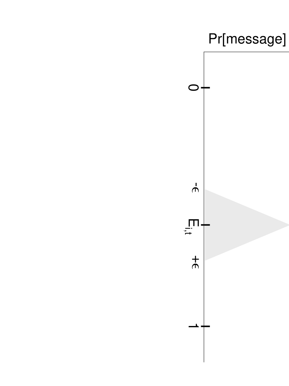
The reader might be wondering why we chose triangular noise, and whether other types of noise would work equally well. The answer is that we want the message distribution to have three basic properties. First, it should be concentrated about a mean of with variance at most ˜. Second, shifting the mean by should shift the distribution by at most ˜ in variation distance. And third, the derivative of the probably density function should never exceed ˜ in absolute value. Thus, Gaussian noise would also work, though it is somewhat harder to analyze than triangular noise. However, noise that is uniform over would not work (so far as we could tell), since it violates the third property.
Before we analyze the protocol, we need to develop some notation. Let consist of the first messages that Alice and Bob exchange. Since messages are now probabilistic, the agents’ expectations of at step depend not only on the initial state of the world , but also on . When we want to emphasize this, we denote the agents’ expectations by and respectively. Another important consequence of messages being probabilistic is that after an agent has received a message, its posterior distribution over is no longer obtainable by restricting the prior distribution to a subset of possible states. Thus, we let , since we will never refer to for .
Say the agents -agree after the message if
Also, let
Theorem 11
For all , the smoothed standard protocol causes Alice and Bob to -agree after at most messages.
Proof. Similarly to Theorem 6, we let be the expectation of a third party Charlie who sees all messages between Alice and Bob, but who knows neither their inputs nor the random bits that they use to produce their messages. We then track .
Assume that and that Alice sends the message . Notice that cannot deviate from Alice’s expectation by more than , since and . So keeping fixed,
for all . Now Charlie’s expectation is just an average of ’s, so it follows that
as well. Similarly, after Bob sends the message,
Therefore
using the triangle inequality and the fact that . The final observation is that Charlie’s partition of at step refines his partition at step , so by Proposition 4,
Since , this yields an upper bound of on the number of messages.
4.2 Simulating the Smoothed Protocol
Having proved that the smoothed standard protocol works, in this section we explain how Alice and Bob can simulate the protocol. In the ideal case—where the agents have unlimited computational power—they use the following recursive formulas. Let
be proportional to the probability that agent sends message , given that its expectation is . Also, let be proportional to the joint probability of messages assuming the true state of the world is . Then assuming is even and suppressing dependencies on , for all we have
with the base cases for all . The correctness of these formulas follows from simple Bayesian manipulations. Having computed by the formulas above (note that this does not require knowledge of ), all agent needs to do is draw from the triangular distribution, then send the message
In the real case, the agents are computationally bounded, and can no longer afford the luxury of taking expectations over the exponentially large sets . A natural idea is to compensate by somehow sampling those sets. But since we never assumed the ability to sample conditioned on messages , it is not obvious how that make that idea work. Our solution will consist of two phases: the construction of “sampling-trees,” which involves no communication, followed by a message-by-message simulation of the ideal protocol. Let us describe these phases in turn.
(I) Sampling-Tree Construction. Alice creates a tree with height and branching factor . Here is the number of messages, and is a parameter to be specified later. Let be the root node of , and let be the set of children of node . Then Alice labels each of the nodes by a sample , drawn independently from her posterior distribution . Next, for each , she labels each of the nodes by a sample , drawn independently from Bob’s distribution where . She continues recursively in this manner, labeling each an even distance from the root with a sample where is the parent of , and each an odd distance from the root with a sample where is the parent of . Thus her total number of samples is
Similarly, Bob creates a tree with height and branching factor . Let be the root of ; then Bob labels each by a sample , each child of each by a sample , and so on, alternating between and at successive levels. As a side remark, if the agents share a random string, then there is no reason for them not to use the same set of samples. However, we cannot assume that such a string is available.
(II) Simulation. We now explain how the agents can use the samples from (I) to simulate the smoothed standard protocol. First Alice estimates her expectation by the quantity
She then chooses a random and sends Bob
On receiving the message, for each Bob computes
his estimate of assuming . He then defines
and estimates his own expectation by
Finally, he chooses a random and sends Alice
In general, if is even then the recursive formulas for agent are
with the base cases for all . Agent computes a message in the obvious way, from its expectation at the root of :
That completes the description of the simulation procedure. Its complexity is easily determined: let be the number of computational steps needed to sample from or , and let be number of steps needed to evaluate . Then both agents use steps, where we have summed over all communication rounds. Thus, the complexity is exponential in ; on the other hand, it has no dependence on .
4.3 Analysis
Our goal is to show that the message sequence in the simulated protocol is statistically indistinguishable from the sequence in the ideal protocol, for some reasonable sample size . Here ‘reasonable’, unfortunately, is still quite huge: of order , where is the maximum bias with which a referee can distinguish the conversations. So assuming and , the total number of computational steps is of order
The reader might complain that this bound is not at all reasonable: for example, if , then it translates into more than subroutine calls! Let us make two points in response. First, we do show that the number of subroutine calls needed is independent of , and that it grows “only” exponentially in a polynomial in and . Theoretical computer scientists often see cases in which the first polynomial-time algorithm for a problem has a completely impractical complexity, say . However, once the problem is known to be in polynomial time, it is usually possible to reduce the exponent to obtain a truly practical algorithm. In our case, we conjecture that the factor of in the exponent could be reduced to or even ; certainly the constants in the exponent can be reduced. The second point is that the complexity is so large only because we never assumed the agents can sample from their sets of possible states conditioned on messages exchanged. So the best they can do is to sample a huge number of states from their original sets and , then retain the few that are compatible with the messages. However, it seems likely that agents would have at least some ability to sample conditioned on messages. After all, we assumed that they enter the conversation with the ability to sample, and presumably they have had other conversations in the past! In practice, then, the complexity will probably be better than the worst-case estimate above.
How do we prove the simulation theorem? In one sense, the proof is ‘merely’ an exercise in error analysis and large deviation bounds. However, the details are extremely subtle and difficult to get right. The problem is that if a message has probability from its recipient’s point of view, then order samples are needed to find even a single input that could have caused the sender to produce that message. Fortunately, low-probability messages are unlikely to be sent, for almost tautological reasons that we spell out in Lemma 14. However, because the sample trees are so large, with overwhelming probability they contain some nodes with miniscule values of . We need to argue that the errors introduced by these “bad nodes” are washed out by the good nodes before they can propagate to the root.
The proof will repeatedly use the Chernoff-Hoeffding bound (Theorem 2). As shown by the following corollary, Theorem 2 sometimes lets us estimate the mean of a random variable, even if we cannot sample that variable directly.
Corollary 12
Let and belong to , and let and . If we choose indices uniformly at random from , then
We will also need a bound for a sum of exponentially distributed variables, which can be found in [6] for example.
Theorem 13
Let be independent and exponentially distributed with mean (that is, ). Then
For convenience, we will state our results in terms of Alice’s tree , with the understanding that they apply equally well to . Throughout, we assume that is even and that the message is sent from Bob to Alice. Let measure the “likelihood” of Alice’s situation at step . Then measures the likelihood of the message, conditioned on Alice’s situation just before she receives it. The following lemma says essentially that “unlikely messages are unlikely.”
Lemma 14
For all inputs of Alice, message sequences , and constants ,
Proof. For all ,
from Alice’s point of view. So it suffices to observe that
Here the first inequality follows from elementary probability theory, together with the fact that there are at most possible messages , and hence the mean of over chosen uniformly at random is at least
The second inequality follows since .
A consequence of Lemma 14 is that unlikely sequences of messages are unlikely. For the remainder of this section, let .
Lemma 15
For all and all ,
Proof. For all , let . Then
since . Furthermore, Lemma 14 implies that for each ,
even conditioned on . Therefore is stochastically dominated by a sum of independent exponential variables each with mean . So by Theorem 13,
Setting and solving to obtain , it follows that
In the next four results, we fix a particular node , then study how the error at depends on the errors at its children . For simplicity, we assume is an even distance from the root, but our results will apply equally to nodes an odd distance from the root. We need to upper-bound the expected difference between Alice’s actual expectation , and her ideal expectation . To this end, it will be helpful to define the following “hybrid” between and :
To compute , we use the ideal weights , but we average over Alice’s samples only, not over all of . By the triangle inequality, to upper-bound it suffices to upper-bound and . We start with the latter.
Lemma 16
Proof. Assuming ,
by Corollary 12. Furthermore, since and are in , we have the trivial but important bound . Therefore
Here the fifth line uses Lemma 15, and
By straightforward integral approximations, the last expression is at most for sufficiently large .
For each child , let
measure the total error in Alice’s estimates of , summed over all time steps . The following proposition shows that to upper-bound the error in , it suffices to upper-bound . For this proposition to hold, we need the function to have bounded derivative. That is why we chose triangular instead of uniform noise when defining the protocol.
Proposition 17
Proof. From the definition of ,
Furthermore, and are both bounded in . It follows that
where ranges over .
Now let
so that and . Using Lemma 15, we can upper-bound the probability that is too much smaller than its mean value.
Corollary 18
For all ,
Proof. By the principle of deferred decisions, we can think of each as an independent sample of a random variable with mean . Then is a sum of such samples. Setting , by Lemma 15 we have
Furthermore, assuming , Theorem 2 yields
The corollary now follows by the union bound.
The last piece of the puzzle is to upper-bound the difference between and , using techniques similar to those of Lemma 16. Let and .
Lemma 19
Assuming for all ,
Proof. Using the fact that ,
by the same trick as in Corollary 12. Furthermore, it follows from Proposition 17 together with the triangle inequality that and . So we can upper-bound by , as well as (of course) by . Fix ; then
where the second line uses Corollary 18 and . This in turn is at most
Assuming always, the expectation of the above quantity over is at most .
We are finally ready to put everything together, and show that the referee can distinguish the real and ideal conversations with bias at most .
Theorem 20
By setting and , it is possible to achieve
for all Boolean functions .
Proof. Combining Lemmas 16 and 19,
Let be the set of nodes at the level of Alice’s tree . Then if is even, let
By linearity of expectation,
Solving this recurrence relation, we find that at the root node,
and similarly for the root of Bob’s tree . So in particular, for all , where
Now observe that, if we let be the distribution over message in the wannabe case, and let be the distribution in the unbounded Bayesian case, then
where denotes variation distance. So the referee can distinguish the whole conversations with bias at most
since variation distance satisfies the triangle inequality. Therefore, we can achieve the goal of simulation by taking , or equivalently
5 Discussion
“We publish this observation with some diffidence, since once one has the appropriate framework, it is mathematically trivial. Intuitively, though, it is not quite obvious…” —Aumann [2], on his original agreement result
This paper has studied agreement protocols from the quantitative perspective of theoretical computer science. If nothing else, we hope to have shown that adopting that perspective leads to rich mathematical questions. Here are a few of the more interesting open problems raised by our results:
- •
How tight is our upper bound? Can we improve Theorem 6 to show that the discretized standard protocol uses only messages, independently of ? More importantly, is there a scenario where Alice and Bob must exchange or bits to -agree, regardless of what protocol they use? Recall that the best lower bound we currently know is , from Proposition 3.
- •
Can Alice and Bob -agree after a small number of steps, even if the “true” distribution over differs from their shared prior distribution ? Or is there a scenario where regardless of what protocol they use, there exists a state for which they must exchange bits to agree within on ? (It is easy to construct a scenario where the discretized standard protocol needs bits for some .)
- •
Can the simulation procedure of Section 4.2 be made practical? That is, can we reduce the number of subroutine calls to (say) , or even to a polynomial in and ? Alternatively, can we prove a lower bound showing that such reductions are impossible?
- •
Can we obtain a better simulation procedure if is represented in a compact form, for example a graphical model?
Stepping back, have the results of this paper taught us anything about the origins of disagreement? As mentioned in Section 1, it is easy to list plausible reasons why people might disagree, Aumann’s theorem notwithstanding: indifference to truth, misconstrual, vagueness, dishonesty, self-deceit, mistrust, stupidity, systematic cognitive biases, no priors, different priors, different indexicality assumptions, diagonalization (as discussed in Section 3), communication cost, and computation cost, among others. But which of these reasons, if any, are fundamental? In other words, were we forced to identify a single point at which the assumptions of Aumann’s theorem diverge from reality, what would it be?
Before we undertook the research described in this paper, we would have said either that
- (1)
imposing reasonable communication and computation bounds is likely to change everything, or
- (2)
at least one party to any persistent disagreement must be dishonest, irrational, or indifferent to truth.66 6 Here “indifference to truth” means choosing opinions according to their novelty, social acceptability, value in attracting sexual partners, etc. rather than evidence.
Today, however, we would make an argument less technical than (1) and less misanthropic than (2): that even in idealized models, we should not treat agents as initially-identical Bayesian “containers” that later get filled with different experiences. In particular, the Common Prior Assumption (CPA) is fundamentally misguided.
Presumably no one would claim that the CPA is empirically true for human beings. It seems obvious that, when five-year-olds go to Sunday school, they are not updating a shared prior over possible religions conditioned on what their teacher tells them. Rather, their priors are being “initialized” to some extent. Furthermore, the existence of a common prior would be astonishing from the perspectives of physics, evolutionary biology, and neuroscience, since nothing in those fields predicts or requires one. However, as Aumann [3] rightly emphasizes, the question is not whether the CPA is “true” but whether it is a useful idealization. What we suggest is that, when trying to understand the origins of disagreement, the CPA is not a useful idealization. There are two main reasons for this.
First, the CPA presents difficulties with transtemporal identity. Are you really the “same” person as you were when you were two months old? If not, then why must your posterior be obtained by updating the two-month-old’s prior? The difficulties become even more severe if we adopt the many-worlds view of quantum mechanics. For then there are millions of basis states containing beings very much like you. Suppose we fix which one of those beings is “really” you at time ; then which one is you at times or ? Quantum mechanics does not fix an answer; more than that, it does not even fix the probabilities of possible answers.77 7 What quantum mechanics does fix are the probabilities of possible outcomes of a measurement. But those probabilities will only be meaningful to you if you are not part of the system being measured. That is why Bohmian mechanics and its many variants can all be compatible with quantum mechanics, despite having different equations of motion.
Second, the CPA begs the question of what determines the common prior. Some might argue that human beings’ shared genetic heritage causes them (or rather, should cause them) to share a prior. But if your prior is to fix your initial opinions about everything, then it must assign a probability to your future experiences being consistent with those of (say) a five-legged extraterrestrial. Presumably that probability decreases dramatically once you condition on the indexical fact of your humanity. But it ought to start nonzero and stay nonzero, for instance because of quantum fluctuations. This raises a question: why shouldn’t your prior equal the extraterrestrial’s? After all, the extraterrestrial has to assign a probability to its future experiences being consistent with yours—and at a hypothetical time before either of you knows who “you” will become, why should the two of you reason differently? We can similarly imagine beings governed by different laws of physics; and these, too, should share our prior. It follows that “the” common prior, if it exists, is not determined by anything in our genetic makeup or even the physical world.
This leaves the possibility that mathematics or logic could determine the common prior. Along these lines, Schmidhuber [17] has advocated a prior in which the probability of any sequence of experiences is proportional to , where is the Kolmogorov complexity of —that is, the length of the shortest computer program that outputs . This idea has several problems, though. First, our actual experiences seem to have gratuitously high Kolmogorov complexity. Believers in the Kolmogorov prior are forced to say, without evidence, that this is an illusion. Second, why should we use Kolmogorov complexity, rather than (say) time-bounded Kolmogorov complexity, or perhaps the length of the shortest program that outputs given an oracle for the halting problem? Third, whenever we wish to compare the probabilities of a few “equally complex” events, the probabilities will depend less on the events themselves than on our choice of programming language, so we face another arbitrary choice.
So it seems that a common prior would be independent of the physical world and even of mathematics, yet would somehow be readily available to and unquestioningly accepted by every rational agent. Agents equipped with this prior would live a ‘preprogrammed’ existence, meaning that they would never change, only conditionalize. We have argued that this picture of the world presents serious intrinsic problems, even setting aside its naked implausibility. So perhaps the common prior should be jettisoned with the ether.
But is there any principled basis for prior differences, then? Consider Shakespeare’s Julius Caesar, debating whether to venture outside on the Ides of March. From his dismissals of omens, we know that Caesar bases his final decision on a belief that he will not be in particular danger, rather than just a preference for risky actions. Yet the process of reaching the belief seems to have nothing to do with conditioning on evidence—or rather, it starts after the conditioning is already done. Our proposal is to view the process as that of Caesar choosing his prior, and thereby choosing what sort of person he is. In other words, Caesar assigns a low prior probability to his getting killed, for the sole reason that had he assigned a high one, he would no longer be Caesar but someone else.88 8 [D]anger knows full well That Caesar is more dangerous than he: We are two lions litter’d in one day, And I the elder and more terrible… —Julius Caesar, Act 2, Scene 2 On this view, not only can Alice and Bob have different priors because they are different people, but the fact that they have different priors is a large part of what makes them different people, rather than the same person filling two pairs of shoes.
In saying this, we are not taking the relativist stance that any prior is “rational” for the sort of person who would hold that prior. If no priors are objectively more rational than others, then the word “rational” is meaningless, since there exists a prior to justify essentially any belief. But the question remains: is the number of rational priors exactly one? We have already seen an argument of Hanson [12] that it should be, based on the concept of a “pre-prior” (that is, a prior over all possible priors). Why should Alice give her own prior any more weight than Bob’s? Our response is simply to point out that there is a tremendous gap between empathizing with someone else’s perspective and adopting it, or between calculating what your expectation would be under someone else’s prior and willing that expectation to be yours. No matter how long she talks to Bob, in the end Alice must confront the irreducible fact of her individuality. As Clarence Darrow famously put it, “I don’t like spinach, and I’m glad I don’t, because if I liked it I’d eat it, and I just hate it.”
6 Acknowledgments
I thank Robin Hanson for correspondence during the early stages of this work, and for his wonderfully disorienting papers which introduced me to the topic. I also thank Ran Raz, Umesh Vazirani, and Ronald de Wolf for helpful conversations.
References
- [1] M. Allais and O. Hagen (eds). Expected Utility Hypotheses and the Allais Paradox, Dordrecht, 1979.
- [2] R. J. Aumann. Agreeing to disagree, Annals of Statistics 4(6):1236–1239, 1976.
- [3] R. J. Aumann. Reply to Gul, Econometrica 66(4):929–938, 1998.
- [4] T. Cowen and R. Hanson. Are disagreements honest?, submitted, 2003.
- [5] P. Cross. Not can but will college teaching be improved?, New Directions for Higher Education, 17:1–15, 1977. Cited by Gilovich [9].
- [6] D. P. Dubhashi and A. Panconesi. Concentration of measure for computer scientists, draft at http://www.cs.unibo.it/˜pancones/master.ps.
- [7] J. Earman. Old evidence, new theories: two unresolved problems in Bayesian confirmation theory, Pacific Philosophical Quarterly 70:323–340, 1989.
- [8] J. D. Geanakoplos and H. M. Polemarchakis. We can’t disagree forever, J. Economic Theory 28:192–200, 1982.
- [9] T. Gilovich. How We Know What Isn’t So, Free Press, 1993.
- [10] F. Gul. A comment on Aumann’s Bayesian view, Econometrica 66(4):923–927, 1998.
- [11] R. Hanson. Disagreement is unpredictable, Economics Letters 77(3):365–369, November 2002.
- [12] R. Hanson. Uncommon priors require origin disputes, submitted, 2004.
- [13] R. Hanson. For savvy Bayesian wannabes, are disagreements not about information?, Theory and Decision 54(2):105–123, 2003.
- [14] E. Kushilevitz and N. Nisan. Communication Complexity, Cambridge, 1996.
- [15] R. Parikh and P. Krasucki. Communication, consensus, and knowledge, J. Economic Theory 52:178–189, 1990.
- [16] S. Russell and P. Norvig. Artificial Intelligence: A Modern Approach (2nd edition), Prentice Hall, 2002.
- [17] J. Schmidhuber. A computer scientist’s view of life, the universe, and everything, in Foundations of Computer Science: Potential - Theory - Cognition (C. Freksa, ed.), pp. 201–208, Springer, 1997.
- [18] A. M. Turing. Computing machinery and intelligence, Mind 59:433–460, 1950.
- [19] A. Tversky and D. Kahneman. Judgment under uncertainty: heuristics and biases, Science 185:1124–1131, 1974. See also D. Kahneman, P. Slovic, and A. Tversky (eds.), Judgment under Uncertainty, Cambridge, 1982.