Layout of Graphs with Bounded Tree-Width Thanks: Submitted October 14, 2002. Revised August 11, 2026. Results in this paper were presented at the GD ’02 [34], FST TCS ’02 [93], and WG ’03 [36] conferences.
Abstract
A queue layout of a graph consists of a total order of the vertices, and a partition of the edges into queues, such that no two edges in the same queue are nested. The minimum number of queues in a queue layout of a graph is its queue-number. A three-dimensional (straight-line grid) drawing of a graph represents the vertices by points in and the edges by non-crossing line-segments. This paper contributes three main results:
(1) It is proved that the minimum volume of a certain type of three-dimensional drawing of a graph is closely related to the queue-number of . In particular, if is an -vertex member of a proper minor-closed family of graphs (such as a planar graph), then has a drawing if and only if has queue-number.
(2) It is proved that queue-number is bounded by tree-width, thus resolving an open problem due to Ganley and Heath (2001), and disproving a conjecture of Pemmaraju (1992). This result provides renewed hope for the positive resolution of a number of open problems in the theory of queue layouts.
(3) It is proved that graphs of bounded tree-width have three-dimensional drawings with volume. This is the most general family of graphs known to admit three-dimensional drawings with volume.
The proofs depend upon our results regarding track layouts and tree-partitions of graphs, which may be of independent interest.
keywords
queue layout, queue-number, three-dimensional graph drawing, tree-partition, tree-partition-width, tree-width, -tree, track layout, track-number, acyclic colouring, acyclic chromatic number.AMS
05C62 (graph representations)1 Introduction
A queue layout of a graph consists of a total order of the vertices, and a partition of the edges into queues, such that no two edges in the same queue are nested. The dual concept of a stack layout, introduced by Ollmann [73] and commonly called a book embedding, is defined similarly, except that no two edges in the same stack may cross. The minimum number of queues (respectively, stacks) in a queue layout (stack layout) of a graph is its queue-number (stack-number). Queue layouts have been extensively studied [41, 53, 54, 58, 76, 80, 86, 88] with applications in parallel process scheduling, fault-tolerant processing, matrix computations, and sorting networks (see [76] for a survey). Queue layouts of directed acyclic graphs [9, 56, 57, 76] and posets [55, 76] have also been investigated. Our motivation for studying queue layouts is a connection with three-dimensional graph drawing.
Graph drawing is concerned with the automatic generation of aesthetically pleasing geometric representations of graphs. Graph drawing in the plane is well-studied (see [24, 64]). Motivated by experimental evidence suggesting that displaying a graph in three dimensions is better than in two [90, 91], and applications including information visualisation [90], VLSI circuit design [66], and software engineering [92], there is a growing body of research in three-dimensional graph drawing. In this paper we study three-dimensional straight-line grid drawings, or three-dimensional drawings for short. In this model, vertices are positioned at grid-points in , and edges are drawn as straight line-segments with no crossings [17, 21, 25, 27, 28, 42, 53, 78, 75]. We focus on the problem of producing three-dimensional drawings with small volume. Three-dimensional drawings with the vertices in have also been studied [39, 47, 19, 16, 18, 61, 22, 63, 60, 62, 69, 74]. Aesthetic criteria besides volume that have been considered include symmetry [60, 61, 62, 63], aspect ratio [19, 47], angular resolution [47, 19], edge-separation [19, 47], and convexity [18, 19, 39, 87].
The first main result of this paper reduces the question of whether a graph has a three-dimensional drawing with small volume to a question regarding queue layouts (Theorem 10). In particular, we prove that every -vertex graph from a proper minor-closed graph family has a drawing if and only if has a queue-number, and this result holds true when replacing by . Consider the family of planar graphs, which are minor-closed. (In the conference version of their paper) Felsneret al.[42] asked whether every planar graph has a three-dimensional drawing with volume? Heath et al. [58, 54] asked whether every planar graph has queue-number? By our result, these two open problems are almost equivalent in the following sense. If every planar graph has queue-number, then every planar graph has a three-dimensional drawing with volume. Conversely, if every planar graph has a drawing, then every planar graph has queue-number. It is possible, however, that planar graphs have unbounded queue-number, yet have say drawings.
Our other main results regard three-dimensional drawings and queue layouts of graphs with bounded tree-width. Tree-width, first defined by Halin [50], although largely unnoticed until independently rediscovered by Robertson and Seymour [81] and Arnborg and Proskurowski [7], is a measure of the similarity of a graph to a tree (see §2.1 for the definition). Tree-width (or its special case, path-width) has been previously used in the context of graph drawing by Dujmovićet al.[33], Hliněný [59], and Peng [77], for example.
The second main result is that the queue-number of a graph is bounded by its tree-width (). This solves an open problem due to Ganley and Heath [45], who proved that stack-number is bounded by tree-width, and asked whether a similar relationship holds for queue-number. This result has significant implications for the above open problem (does every planar graph have queue-number), and the more general question (since planar graphs have stack-number at most four [94]) of whether queue-number is bounded by stack-number. Heath et al. [58, 54] originally conjectured that both of these questions have an affirmative answer. More recently however, Pemmaraju [76] conjectured that the ‘stellated ’, a planar -tree, has queue-number, and provided evidence to support this conjecture (also see [45]). This suggested that the answer to both of the above questions was negative. In particular, Pemmaraju [76] and Heath [private communication, 2002] conjectured that planar graphs have queue-number. However, our result provides a queue-layout of any -tree, and thus the stellated , with queues. Hence our result disproves the first conjecture of Pemmaraju [76] mentioned above, and renews hope in an affirmative answer to the above open problems.
The third main result is that every graph of bounded tree-width has a three-dimensional drawing with volume. The family of graphs of bounded tree-width includes most of the graphs previously known to admit three-dimensional drawings with volume (for example, outerplanar graphs), and also includes many graph families for which the previous best volume bound was (for example, series-parallel graphs). Many graphs arising in applications of graph drawing do have small tree-width. Outerplanar and series-parallel graphs are the obvious examples. Another example arises in software engineering applications. Thorup [89] proved that the control-flow graphs of go-to free programs in many programming languages have tree-width bounded by a small constant; in particular, for Pascal and for C. Other families of graphs having bounded tree-width (for constant ) include: almost trees with parameter , graphs with a feedback vertex set of size , band-width graphs, cut-width graphs, planar graphs of radius , and -outerplanar graphs. If the size of a maximum clique is a constant then chordal, interval and circular arc graphs also have bounded tree-width. Thus, by our result, all of these graphs have three-dimensional drawings with volume, and queue-number.
To prove our results for graphs of bounded tree-width, we employ a related structure called a tree-partition, introduced independently by Seese [85] and Halin [51]. A tree-partition of a graph is a partition of its vertices into ‘bags’ such that contracting each bag to a single vertex gives a forest (after deleting loops and replacing parallel edges by a single edge). In a result of independent interest, we prove that every -tree has a tree-partition such that each bag induces a connected -tree, amongst other properties. The second tool that we use is a track layout, which consists of a vertex-colouring and a total order of each colour class, such that between any two colour classes no two edges cross.
The remainder of the paper is organised as follows. In §2 we introduce the required background material, and state our results regarding three-dimensional drawings and queue layouts, and compare these with results in the literature. In §3 we establish a number of results concerning track layouts. That three-dimensional drawings and queue-layouts are closely related stems from the fact that three-dimensional drawings and queue layouts are both closely related to track layouts, as proved in §4 and §5, respectively. In §6 we prove the above-mentioned theorem for tree-partitions of -trees, which is used in §7 to construct track layouts of graphs with bounded tree-width. We conclude in §8 with a number of open problems.
2 Background and Results
Throughout this paper all graphs are undirected, simple, and finite with vertex set and edge set . The number of vertices and the maximum degree of are respectively denoted by and . The subgraph induced by a set of vertices is denoted by . For all disjoint subsets , the bipartite subgraph of with vertex set and edge set is denoted by .
A graph is a minor of a graph if is isomorphic to a graph obtained from a subgraph of by contracting edges. A family of graphs closed under taking minors is proper if it is not the class of all graphs.
A graph parameter is a function that assigns to every graph a non-negative integer . Let be a family of graphs. By we denote the function , where is the maximum of , taken over all -vertex graphs . We say has bounded if . A graph parameter is bounded by a graph parameter (for some graph family ), if there exists a function such that for every graph (in ).
2.1 Tree-Width
Let be a graph and let be a tree. An element of is called a node. Let be a set of subsets of indexed by the nodes of . Each is called a bag. The pair is a tree-decomposition of if:
- 1.
(that is, every vertex of is in at least one bag),
- 2.
edge of , node of such that and , and
- 3.
nodes of , if is on the path from to in , then .
The width of a tree-decomposition is one less than the maximum cardinality of a bag. A path-decomposition is a tree-decomposition where the tree is a path , which is simply identified by the sequence of bags where each . The path-width (respectively, tree-width) of a graph , denoted by (), is the minimum width of a path- (tree-) decomposition of . Graphs with tree-width at most one are precisely the forests. Graphs with tree-width at most two are called series-parallel11 1 ‘Series-parallel digraphs’ are often defined in terms of certain ‘series’ and ‘parallel’ composition operations. The underlying undirected graph of such a digraph has tree-width at most two (see [10])., and are characterised as those graphs with no minor (see [10]).
A -tree for some is defined recursively as follows. The empty graph is a -tree, and the graph obtained from a -tree by adding a new vertex adjacent to each vertex of a clique with at most vertices is also a -tree. This definition of a -tree is by Reed [79]. The following more restrictive definition of a -tree, which we call ‘strict’, was introduced by Arnborg and Proskurowski [7], and is more often used in the literature. A -clique is a strict -tree, and the graph obtained from a strict -tree by adding a new vertex adjacent to each vertex of a -clique is also a strict -tree. Obviously the strict -trees are a proper sub-class of the -trees. A subgraph of a -tree is called a partial -tree, and a subgraph of a strict -tree is called a partial strict -tree. The following result is well known (see for example [10, 79]). A chord of a cycle is an edge not in whose end-vertices are both in . A graph is chordal if every cycle on at least four vertices has a chord.
Lemma 1.
Let be a graph. The following are equivalent:
- 1.
has tree-width ,
- 2.
is a partial -tree,
- 3.
is a partial strict -tree,
- 4.
is a subgraph of a chordal graph that has no clique on vertices.
2.2 Tree-Partitions
As in the definition of a tree-decomposition, let be graph and let be a set of subsets of (called bags) indexed by the nodes of a tree . The pair is a tree-partition of if
- 1.
distinct nodes and of , , and
- 2.
edge of , either
- (a)
node of with and ( is called an intra-bag edge), or
- (b)
edge of with and ( is called an inter-bag edge).
- (a)
The main property of tree-partitions that has been studied in the literature is the maximum cardinality of a bag, called the width of the tree-partition [11, 51, 85, 31, 32]. The minimum width over all tree-partitions of a graph is the tree-partition-width22 2 Tree-partition-width has also been called strong tree-width [85, 11]. of , denoted by . A graph with bounded degree has bounded tree-partition-width if and only if it has bounded tree-width [32]. In particular, for every graph , Ding and Oporowski [31] proved that , and Seese [85] proved that .
Theorem 25 provides a tree-partition of a -tree with additional features besides small width. First, the subgraph induced by each bag is a connected -tree. This allows us to perform induction on . Second, in each non-root bag the set of vertices in the parent bag of with a neighbour in form a clique. This feature is crucial in the intended application (Theorem 28). Finally the tree-partition has width at most , which represents a constant-factor improvement over the above result by Ding and Oporowski [31] in the case of -trees.
2.3 Track Layouts
Let be a graph. A colouring of is a partition of , where is a set of colours, such that for every edge of , if and then . Each set is called a colour class. A colouring of with colours is a -colouring, and we say that is -colourable. The chromatic number of , denoted by , is the minimum such that is -colourable.
If is a total order of a colour class , then we call the pair a track. If is a colouring of , and is a track, for each colour , then we say is a track assignment of indexed by . Note that at times it will be convenient to also refer to a colour and the colour class as a track. The precise meaning will always be clear from the context. A -track assignment is a track assignment with tracks.
As illustrated in Fig. 1, an X-crossing in a track assignment consists of two edges and such that and , for distinct tracks and . A -track assignment with no X-crossing is called a -track layout. The track-number of a graph , denoted by , is the minimum such that has a -track layout.

Let be a -track layout of a graph . The span of an edge of , with respect to a numbering of the tracks , is defined to be where and .
Track layouts will be central in most of our proofs. To enable comparison of our results to those in the literature we now introduce the notion of an ‘improper’ track layout. A improper colouring of a graph is simply a partition of . Here adjacent vertices may be in the same colour class. A track of an improper colouring is defined as above. Suppose is an improper colouring of , and is a track, for each colour . An edge with both end-vertices in the same track is called an intra-track edge; otherwise it is called an inter-track edge. We say is an improper track assignment of if, for all intra-track edges with and for some , there is no vertex with . That is, adjacent vertices in the same track are consecutive in that track. An improper -track assignment with no X-crossing is called an improper -track layout33 3 In [34, 35, 93] we called a track layout an ordered layering with no X-crossing and no intra-layer edges, and an improper track layout was called an ordered layering with no X-crossing..
Lemma 2.
If a graph has an improper -track layout, then has a -track layout.
Proof.
For every track of an improper -track layout of , let be a new track. Move every second vertex from to , such that inherits its total order from the original . Clearly there is no intra-track edge and no X-crossing. Thus we obtain a -track layout of . ∎
Hence the track-number of a graph is at most twice its ‘improper track-number’. The following lemma, which was jointly discovered with Giuseppe Liotta, gives a compelling reason to only consider proper track layouts. Similar ideas can be found in [42, 27]. Let be an edge of a graph . Let be the graph obtained from by adding a new vertex only adjacent to and . We say is an ear, and is obtained from by adding an ear to .
Lemma 3.
Let be a class of graphs closed under the addition of ears (for example, series-parallel graphs or planar graphs). If every graph in has an improper -track layout for some constant , then every graph in has a (proper) -track layout.
Proof.
For any graph , let be the graph obtained from by adding ears to every edge of . By assumption, has an improper -track layout. Suppose that there is an edge of such that and are in the same track. None of the ears added to are on the same track, as otherwise adjacent vertices would not be consecutive in that track. Thus there is a track containing at least two of the ears added to . However, this implies that there is an X-crossing, which is a contradiction. Thus the end-vertices of every edge of are in distinct tracks. Hence the improper -track layout of contains a -track layout of . ∎
Lemmata 2 and 3 imply that only for relatively small classes of graphs will the distinction between track layouts and improper track layouts be significant. We therefore chose to work with the less cumbersome notion of a track layout. The following theorem summarises our bounds on the track-number of a graph.
Theorem 4.
Let be a graph with maximum degree , path-width , tree-partition-width , and tree-width . The track-number of satisfies:
- (a)
,
- (b)
,
- (c)
.
2.4 Vertex-Orderings
Let be a graph. A total order of is called a vertex-ordering of . Suppose is connected. The depth of a vertex in is the graph-theoretic distance between and in . We say is a breadth-first vertex-ordering if for all vertices and with , the depth of in is no more than the depth of in . Vertex-orderings, and in particular, vertex-orderings of trees will be used extensively in this paper. Consider a breadth-first vertex-ordering of a tree such that vertices at depth are ordered with respect to the ordering of vertices at depth . In particular, if and are vertices at depth with respective parents and at depth with then . Such a vertex-ordering is called a lexicographical breadth-first vertex-ordering of , and is illustrated in Fig. 2.

2.5 Queue Layouts
A queue layout of a graph consists of a vertex-ordering of , and a partition of into queues, such that no two edges in the same queue are nested with respect to . That is, there are no edges and in a single queue with . The minimum number of queues in a queue layout of is called the queue-number of , and is denoted by . A similar concept is that of a stack layout (or book embedding), which consists of a vertex-ordering of , and a partition of into stacks (or pages) such that there are no edges and in a single stack with . The minimum number of stacks in a stack layout of is called the stack-number (or page-number or book-thickness) of , and is denoted by . A queue (respectively, stack) layout with queues (stacks) is called a -queue (-stack) layout, and a graph that admits a -queue (-stack) layout is called a -queue (-stack) graph.
Heath and Rosenberg [58] characterised -queue graphs as the ‘arched levelled planar’ graphs, and proved that it is -complete to recognise such graphs. This result is in contrast to the situation for stack layouts — 1-stack graphs are precisely the outerplanar graphs [8], which can be recognised in polynomial time. Heathet al.[54] proved that 1-stack graphs are -queue graphs (rediscovered by Rengarajan and Veni Madhavan [80]), and that -queue graphs are -stack graphs.
While it is -hard to minimise the number of stacks in a stack layout given a fixed vertex-ordering [46], the analogous problem for queue layouts can be solved as follows. A -rainbow in a vertex-ordering consists of a matching such that , as illustrated in Fig. 3.

A vertex-ordering containing a -rainbow needs at least queues. A straightforward application of Dilworth’s Theorem [30] proves the converse. That is, a fixed vertex-ordering admits a -queue layout where is the size of the largest rainbow. (Heath and Rosenberg [58] describe a time algorithm to compute the queue assignment.) Thus determining can be viewed as the following vertex-ordering problem.
Lemma 5 ([58]).
The queue-number of a graph is the minimum, taken over all vertex-orderings of , of the maximum size of a rainbow in .
Stack and/or queue layouts of -trees have previously been investigated in [20, 80, 45]. A -tree is a -queue graph, since in a lexicographical breadth-first vertex-ordering of a tree no two edges are nested (see Fig. 2). Chunget al.[20] proved that in a depth-first vertex-ordering of a tree no two edges cross. Thus -trees are -stack graphs. Rengarajan and Veni Madhavan [80] proved that graphs with tree-width at most two (the series parallel graphs) are -stack and -queue graphs44 4 In [35] we give a simple proof based on Theorem 25 for the result by Rengarajan and Veni Madhavan [80] that every series-parallel graph has a -queue layout.. Improper track layouts are implicit in the work of Heathet al.[54] and Rengarajan and Veni Madhavan [80]. In §5 we prove the following fundamental relationship between queue and track layouts.
Theorem 6.
For every graph , . Moreover, if is any proper minor-closed graph family, then has queue-number if and only if has track-number , where is any family of functions closed under multiplication (such as or ).
Ganley and Heath [45] proved that every graph has stack-number (using a depth-first traversal of a tree-decomposition), and asked whether queue-number is bounded by tree-width? One of the principal results of this paper is to solve this question in the affirmative. Applying Theorems 4 and 6 we have the following.
Theorem 7.
Let be a graph with maximum degree , path-width , tree-partition-width , and tree-width . The queue-number satisfies55 5 In [93] we obtained an alternative proof that using the ‘vertex separation number’ of a graph (which equals its path-width), and applying Lemma 5 directly we proved that , and thus .:
- (a)
,
- (b)
,
- (c)
.
A similar upper bound to Theorem 7(a) is obtained by Heath and Rosenberg [58], who proved that every graph has , where is the band-width of . In many cases this result is weaker than Theorem 7(a) since (see [29]). More importantly, we have the following corollary of Theorem 7(c).
Corollary 8.
Queue-number is bounded by tree-width, and hence graphs with bounded tree-width have bounded queue-number.
2.6 Three-Dimensional Drawings
A three-dimensional straight-line grid drawing of a graph, henceforth called a three-dimensional drawing, represents the vertices by distinct points in (called grid-points), and represents each edge as a line-segment between its end-vertices, such that edges only intersect at common end-vertices, and an edge only intersects a vertex that is an end-vertex of that edge.
In contrast to the case in the plane, a folklore result states that every graph has a three-dimensional drawing. Such a drawing can be constructed using the ‘moment curve’ algorithm in which vertex , , is represented by the grid-point . It is easily seen — compare with Lemma 21 — that no two edges cross. (Two edges cross if they intersect at some point other than a common end-vertex.)
Since every graph has a three-dimensional drawing, we are interested in optimising certain measures of the aesthetic quality of a drawing. If a three-dimensional drawing is contained in an axis-aligned box with side lengths , and , then we speak of an drawing with volume and aspect ratio . This paper considers the problem of producing a three-dimensional drawing of a given graph with small volume, and with small aspect ratio as a secondary criterion.
Observe that the drawings produced by the moment curve algorithm have volume. Cohenet al.[21] improved this bound, by proving that if is a prime with , and each vertex is represented by the grid-point , then there is still no crossing. This construction is a generalisation of an analogous two-dimensional technique due to Erdős [40]. Furthermore, Cohenet al.[21] proved that the resulting volume bound is asymptotically optimal in the case of the complete graph . It is therefore of interest to identify fixed graph parameters that allow for three-dimensional drawings with small volume.
The first such parameter to be studied was the chromatic number [17, 75]. Calamoneri and Sterbini [17] proved that every -colourable graph has a three-dimensional drawing with volume. Generalising this result, Pachet al.[75] proved that graphs of bounded chromatic number have three-dimensional drawings with volume, and that this bound is asymptotically optimal for the complete bipartite graph with equal sized bipartitions. If is a suitably chosen prime, the main step of this algorithm represents the vertices in the th colour class by grid-points in the set . It follows that the volume bound is for -colourable graphs.
The lower bound of Pachet al.[75] for the complete bipartite graph was generalised by Boseet al.[14] for all graphs. They proved that every three-dimensional drawing with vertices and edges has volume at least . In particular, the maximum number of edges in an drawing is exactly . For example, graphs admitting three-dimensional drawings with volume have edges.
The first non-trivial volume bound was established by Felsneret al.[42] for outerplanar graphs. Their elegant algorithm ‘wraps’ a two-dimensional drawing around a triangular prism to obtain an improper -track layout (see Lemmata 15 and 18 for more on this method). Poranen [78] proved that series-parallel digraphs have upward three-dimensional drawings with volume, and that this bound can be improved to and in certain special cases. Di Giacomo [27] proved that series-parallel graphs with maximum degree three have three-dimensional drawings with volume.
In §4 we prove the following intrinsic relationship between three-dimensional drawings and track layouts.
Theorem 9.
Every graph has a drawing. Moreover, has a drawing if and only if has track-number , where is a family of functions closed under multiplication.
Of course, every graph has an -track layout — simply place a single vertex on each track. Thus Theorem 9 matches the volume bound discussed in §2.6. In fact, the drawings of produced by our algorithm, with each vertex in a distinct track, are identical to those produced by the algorithm of Cohenet al.[21].
Theorems 6 and 9 immediately imply the following result, which reduces the problem of producing a three-dimensional drawing with small volume to that of producing a queue layout of the same graph with few queues.
Theorem 10.
Let be a proper minor-closed family of graphs, and let be a family of functions closed under multiplication. The following are equivalent:
- (a)
every -vertex graph in has a drawing,
- (b)
has track-number , and
- (c)
has queue-number .
Graphs with constant queue-number include de Bruijn graphs, FFT and Beneš network graphs [58]. By Theorem 10, these graphs have three-dimensional drawings with volume. Applying Theorems 4 and 9 we have the following result.
Theorem 11.
Let be a graph with maximum degree , path-width , tree-partition-width , and tree-width . Then has a three-dimensional drawing with the following dimensions:
- (a)
, which is ,
- (b)
, which is ,
- (c)
.
Most importantly, we have the following corollary of Theorem 11(c).
Corollary 12.
Every graph with bounded tree-width has a three-dimensional drawing with volume.
Note that bounded tree-width is not necessary for a graph to have a three-dimensional drawing with volume. The plane grid graph has tree-width, and has a drawing with volume. It also has a -track layout, and thus, by Lemma 21, has a drawing.
Since a planar graph is -colourable, by the results of Calamoneri and Sterbini [17] and Pach [75] discussed above, every planar graph has a three-dimensional drawing with volume. This result also follows from the classical algorithms of de Fraysseixet al.[23] and Schnyder [84] for producing plane grid drawings. All of these methods produce drawings, which have aspect ratio. Since every planar graph has [10], we have the following corollary of Theorem 11(a).
Corollary 13.
Every planar graph has a three-dimensional drawing with volume and aspect ratio.
This result matches the above volume bounds with an improvement in the aspect ratio by a factor of . As discussed in §1, it is an open problem whether every planar graph has a three-dimensional drawing with volume. Subsequent to this research, Dujmović and Wood [37] proved that graphs excluding a clique minor on a fixed number of vertices, such as planar graphs, have three-dimensional drawings with volume, as do graphs with bounded degree.
Our final result regarding three-dimensional drawings, which is proved in §4, examines the apparent trade-off between aspect ratio and volume.
Theorem 14.
For every graph and for every , , has a three-dimensional drawing with volume and aspect ratio .
3 Track Layouts
In this section we describe a number of methods for producing and manipulating track layouts. The following result is implicit in the proof by Felsneret al.[42] that every outerplanar graph has an improper -track layout.
Lemma 15 ([42]).
Every tree has a -track layout.
Proof.
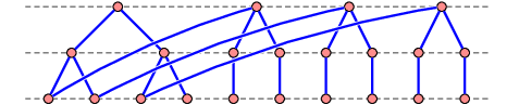
Root at an arbitrary node . Let be a lexicographical breadth-first vertex-ordering of starting at , as described in §2.4. For , let be the set of nodes of with depth in . With each ordered by , we have a -track assignment of . Clearly adjacent vertices are on distinct tracks. Since no two edges are nested in , there is no X-crossing (see Fig. 4). ∎
Lemma 16.
Every graph with path-width has track-number .
Proof.
Let . It is well known that a is the subgraph of a -colourable interval graph [10, 48]. That is, there is a set of intervals such that for every edge of . Let be a -colouring of . Consider each colour class to be an ordered track , where . Suppose there is an X-crossing between edges and with and for some pair of tracks and . Without loss of generality, and . Since is an edge, . Thus , which implies that is not an edge of . This contradiction proves that there is no X-crossing, and has a -track layout. ∎
The next lemma uses a tree-partition to construct a track layout.
Lemma 17.
Every graph with maximum degree , tree-width , and tree-partition-width , has track-number .
Proof.
Let be a tree-partition of with width . By Lemma 15, has a -track layout. Replace each track by ‘sub-tracks’, and for each node in , place the vertices in bag on the sub-tracks replacing the track containing , with at most one vertex in in a single track. For all nodes and of , if in a single track of the -track layout of , then for all vertices and , whenever and are assigned to the same track. There is no X-crossing, since in the track layout of , adjacent nodes are on distinct tracks and there is no X-crossing. Thus we have a track layout of . The number of tracks is , which is at most by the theorem of Ding and Oporowski [31] discussed in §2.2. ∎
In the remainder of this section, we prove two results that show how track layouts can be manipulated without introducing an X-crossing. The first is a generalisation of the ‘wrapping’ algorithm of Felsneret al.[42], who implicitly proved the case .
Lemma 18.
If a graph has an (improper) track layout with maximum edge span , then has an (improper) -track layout.
Proof.
Let . Construct an -track assignment of by merging the tracks for each , , with vertices in appearing before vertices in in the new track , for all with . The given order of each is preserved in the new tracks. It remains to prove that there is no X-crossing. Consider two edges and . Let and , , be the minimum and maximum tracks containing , , or in the given -track layout of .
First consider the case that . Then without loss of generality is in track and is in track . Thus is in a greater track than , and even if (or ) appear on the same track as (or ) in the new -track assignment, (or ) will be to the left of (or ). Thus these edges do not form an X-crossing in the -track assignment. Otherwise . Thus any two of , , or will appear on the same track in the -track assignment if and only if they are on the same track in the given -track layout (since ). Hence the only way for these four vertices to appear on exactly two tracks in the -track assignment is if they were on exactly two layers in the given -track layout, in which case, by assumption and do not form an X-crossing. Therefore there is no X-crossing, and we have an -track layout of . ∎
The next result shows that the number of vertices in different tracks of a track layout can be balanced without introducing an X-crossing. The proof is based on an idea due to Pachet al.[75] for balancing the size of the colour classes in a colouring.
Lemma 19.
If a graph has an (improper) -track layout, then for every , has an (improper) -track layout with at most vertices in each track.
Proof.
For each track with vertices, replace it by ‘sub-tracks’ each with exactly vertices except for at most one sub-track with vertices, such that the vertices in each sub-track are consecutive in the original track, and the original order is maintained. There is no X-crossing between sub-tracks from the same original track as there is at most one edge between such sub-tracks. There is no X-crossing between sub-tracks from different original tracks as otherwise there would be an X-crossing in the original. There are at most tracks with vertices. Since there are at most tracks with less than vertices, one for each of the original tracks, there is a total of at most tracks. ∎
4 Three-Dimensional Drawings and Track Layouts
In this section we prove Theorem 9, which states that three-dimensional drawings with small volume are closely related to track layouts with few tracks.
Lemma 20.
If a graph has an drawing, then has an improper -track layout, and has a -track layout.
Proof.
Let be the set of vertices of with an -coordinate of and a -coordinate of , where without loss of generality and . With each set ordered by the -coordinates of its elements, is an improper -track assignment. There is no X-crossing, as otherwise there would be a crossing in the original drawing, and hence we have an improper -track layout. By Lemma 2, has a -track layout. ∎
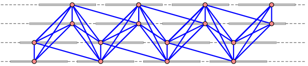
We now prove the converse of Lemma 20. The proof is inspired by the generalisations of the moment curve algorithm by Cohenet al.[21] and Pachet al.[75], described in §2.6. Loosely speaking, Cohenet al.[21] allow three ‘free’ dimensions, whereas Pachet al.[75] use the assignment of vertices to colour classes to ‘fix’ one dimension with two dimensions free. We use an assignment of vertices to tracks to fix two dimensions with one dimension free. The style of three-dimensional drawing produced by our algorithm, where tracks are drawn vertically, is illustrated in Fig. 6.

Lemma 21.
If a graph has a (possibly) improper -track layout, then has a three-dimensional drawing, where is the maximum number of vertices in a track.
Proof.
Suppose is the given improper -track layout. Let be the smallest prime such that . Then by Bertrand’s postulate. For each , , represent the vertices in by the grid-points
such that the -coordinates respect the given total order . Draw each edge as a line-segment between its end-vertices. Suppose two edges and cross such that their end-vertices are at distinct points , . Then these points are coplanar, and if is the matrix
then the determinant . We proceed by considering the number of distinct tracks .
: By the definition of an improper track layout, and do not cross.
: If either edge is intra-track then and do not cross. Otherwise neither edge is intra-track, and since there is no X-crossing, and do not cross.
: Without loss of generality . It follows that , where
Since , . However, is a Vandermonde matrix modulo , and thus
which is non-zero since , and are distinct and is a prime, a contradiction.
: Let be the matrix obtained from by taking each entry modulo . Then . Since , ,
Since each , is a Vandermonde matrix modulo , and thus
which is non-zero since and is a prime. This contradiction proves there are no edge crossings. The produced drawing is at most . ∎
Proof of Theorem 9. Let be a family of functions closed under multiplication. Let be an -vertex graph with a -track layout, where . By Lemma 19 with , has a -track layout with at most vertices in each track. By Lemma 21, has a drawing, which is . Conversely, suppose an -vertex graph has a drawing, where . By Lemma 20, has a track layout with tracks.
5 Queue Layouts and Track Layouts
In this section we prove Theorem 6, which states that track and queue layouts are closely related. Our first lemma highlights this fact — its proof follows immediately from the definitions (see Fig. 7).
Lemma 22.
A bipartite graph has a -track layout with tracks and if and only if has a -queue layout such that in the corresponding vertex-ordering, the vertices in appear before the vertices in .

We now show that a queue layout can be obtained from a track layout. This result can be viewed as a generalisation of the construction of a -queue layout of an outerplanar graph by Heathet al.[54] and Rengarajan and Veni Madhavan [80] (with ).
Lemma 23.
If a graph has a (possibly) improper -track layout with maximum edge span (), then , and if the given track layout is not improper, then .
Proof.
First suppose that there are no intra-track edges. Let be the vertex ordering of . Let be the set of edges with span in the given track layout. As in Lemma 22, two edges from the same pair of tracks are nested in if and only if they form an X-crossing in the track layout. Since no two edges form an X-crossing in the track layout, no two edges that are between the same pair of tracks are nested in . If two edges not from the same pair of tracks have the same span then they are not nested in . (This idea is due to Heath and Rosenberg [58].) Thus no two edges are nested in each , and we have an -queue layout of . If there are intra-track edges, then they all form one additional queue in . ∎
We now set out to prove the converse of Lemma 23. It is well known that the subgraph induced by any two tracks of a track layout is a forest of caterpillars [52]. A colouring of a graph is acyclic if every bichromatic subgraph is a forest; that is, every cycle receives at least three distinct colours. Thus a -track layout of a graph defines an acyclic -colouring of . The minimum number of colours in an acyclic colouring of is the acyclic chromatic number of , denoted by . Thus,
Acyclic colourings were introduced by Grünbaum [49], who proved that every planar graph is acyclically -colourable. This result was steadily improved [1, 65, 68] until Borodin [12] proved that every planar graph is acyclically -colourable, which is the best possible bound. Many other graph families have bounded acyclic chromatic number, including graphs embeddable on a fixed surface [2, 3, 6], -planar graphs [13], graphs with bounded maximum degree [5], and graphs with bounded tree-width. A folklore result states that (see [43]). More generally, Nešetřil and Ossona de Mendez [71] proved that every proper minor-closed graph family has bounded acyclic chromatic number. In fact, Nešetřil and Ossona de Mendez [71] proved that every graph has a star -colouring (every bichromatic subgraph is a forest of stars), where is a (small) quadratic function of the maximum chromatic number of a minor of .
Lemma 24.
Every graph with acyclic chromatic number and queue-number has track-number .
Proof.
Let be an acyclic colouring of . Let be the vertex-ordering in a -queue layout of . Consider an edge with , , and . If then is forward, and if then is backward. Consider the edges to be coloured with colours, where each colour class consists of the forward edges in a single queue, or the backward edges in a single queue.
Alon and Marshall [4] proved that given a (not necessarily proper) edge -colouring of a graph , any acyclic -colouring of can be refined to a -colouring so that the edges between any pair of (vertex) colour classes are monochromatic, and each (vertex) colour class is contained in some original colour class. (Nešetřil and Raspaud [72] generalised this result for coloured mixed graphs.) Apply this result with the given acyclic -colouring of and the edge -colouring discussed above. Consider the resulting colour classes to be tracks ordered by . The edges between any two tracks are from a single queue, and are all forward or all backward.
Suppose that there are edges and that form an X-crossing. Since each track is a subset of some , we can assume that , and . Suppose that and are both forward. The case in which and are both backward is symmetric. Thus and . Since and form an X-crossing, and the tracks are ordered by , we have and . Hence . That is, and are nested. This is the desired contradiction, since edges between any pair of tracks are from a single queue. Thus we have a -track layout of . ∎
Proof of Theorem 6. Let be a family of functions closed under multiplication. Let be an -vertex graph from a proper minor-closed graph family . First, suppose that has a -track layout, where . By Lemma 23, has queue-number . Conversely, suppose has queue-number . By the above-mentioned result of Nešetřil and Ossona de Mendez [71], has bounded acyclic chromatic number . By Lemma 24, has a -track layout, where .
6 Tree-Partitions of -Trees
In this section we prove our theorem regarding tree-partitions of -trees mentioned in §2.2. This result forms the cornerstone of the proof of Theorem 28.
Theorem 25.
Let be a -tree with maximum degree . Then has a rooted tree-partition such that for all nodes of ,
- (a)
if is a non-root node of and is the parent node of , then the set of vertices in with a neighbour in form a clique of , and
- (b)
the induced subgraph is a connected -tree.
Furthermore the width of is at most .
Proof.
We assume is connected, since if is not connected then a tree-partition of that satisfies the theorem can be determined by adding a new root node with an empty bag, adjacent to the root node of a tree-partition of each connected component of .
It is well-known that is a connected -tree if and only if has a vertex-ordering , such that for all ,
- 1.
if is the induced subgraph , then is connected and the vertex-ordering of induced by is a breadth-first vertex-ordering of , and
- 2.
the neighbours of in form a clique with (unless in which case ).
In the language of chordal graphs, is a (reverse) ‘perfect elimination’ vertex-ordering and can be determined, for example, by the Lex-BFS algorithm by Roseet al.[82] (also see [48]). Moreover, we can choose to be any vertex in .
Let be a vertex of minimum degree66 6 We choose to have minimum degree to obtain a slightly improved bound on the width of the tree-partition. If we choose to be an arbitrary vertex then the width is at most , and the remainder of Theorem 25 holds. in . Then . Let be a vertex-ordering of with , and satisfying (i) and (ii). By (i), the depth of each vertex in is the same as the depth of in the vertex-ordering of induced by , for all . We therefore simply speak of the depth of . Let be the set of vertices of at depth .
Claim 1.
For all , and for every connected component of , the set of vertices at depth with a neighbour in form a clique of .
Proof.
The claim in trivial for or . Now suppose that . Assume for the sake of contradiction that there are two non-adjacent vertices and at depth , such that has a neighbour in and has a neighbour in . Let be a shortest path between and with its interior vertices in . Let be a shortest path between and with its interior vertices at depth at most . Since the interior vertices of are at depth , there is no edge between an interior vertex of and an interior vertex of . Thus is a chordless cycle of length at least four, contradicting the fact that is chordal (by Lemma 1). ∎
Define a graph and a partition of indexed by the nodes of as follows. There is one node in for every connected component of each , whose bag is the vertex-set of the corresponding connected component. We say and are at depth . Clearly a vertex in a depth- bag is also at depth . The (unique) node of at depth zero is called the root node. Let two nodes and of be connected by an edge if there is an edge of with and . Thus is a ‘graph-partition’.
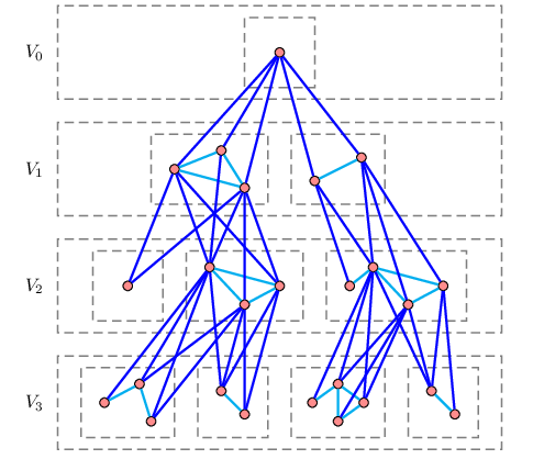
We now prove that in fact is a tree. First observe that is connected since is connected. By definition, nodes of at the same depth are not adjacent. Moreover nodes of can be adjacent only if their depths differ by one. Thus has a cycle only if there is a node in at some depth , such that has at least two distinct neighbours in at depth . However this is impossible since by Claim 1, the set of vertices at depth with a neighbour in form a clique (which we call ), and are hence in a single bag at depth . Thus is a tree and is a tree-partition of (see Fig. 8).
We now prove that each bag induces a connected -tree. This is true for the root node which only has one vertex. Suppose is a non-root node of at depth . Each vertex in has at least one neighbour at depth . Thus in the vertex-ordering of induced by , each vertex has at most neighbours with . Thus the vertex-ordering of induced by satisfies (i) and (ii) for , and is -tree. By definition each is connected.
Finally, consider the cardinality of a bag in . We claim that each bag contains at most vertices. The root bag has one vertex. Let be a non-root node of with parent node . Suppose is the root node. Then , and thus assuming . If then all bags have one vertex. Now assume is a non-root node. The set of vertices in with a neighbour in forms the clique . Let . Thus , and since and is a -tree, . A vertex has neighbours in and at least one neighbour in the parent bag of . Thus has at most neighbours in . Hence the number of edges between and is at most . Every vertex in is adjacent to a vertex in . Thus . This completes the proof. ∎
7 Tree-Width and Track Layouts
In this section we prove that track-number is bounded by tree-width. Let be a track layout of a graph . We say a clique of covers the set of tracks . Let be a set of cliques of . Suppose there exists a total order on such that for all cliques , if there exists a track , and vertices and with , then . In this case, we say is nice, and is nicely ordered by the track layout.
Lemma 26.
Let be a set of tracks in a track layout of a graph . If is a set of cliques, each of which covers , then is nicely ordered by the given track layout.
Proof.
Define a relation on as follows. For every pair of cliques , define if or there exists a track and vertices and with . Clearly all cliques in are comparable.
Suppose that is not antisymmetric; that is, there exists distinct cliques , distinct tracks , and distinct vertices and , such that and . Since and are cliques, the edges and form an X-crossing, which is a contradiction. Thus is antisymmetric.
We claim that is transitive. Suppose there exist cliques such that and . We can assume that , and are pairwise distinct. Thus there are vertices , , and , such that and for some pair of (not necessarily distinct) tracks . Since has a vertex in and since , there is a vertex with . Thus , which implies that . Thus is transitive.
Hence is a total order on , which by definition is nice. ∎
Consider the problem of partitioning the cliques of a graph into sets such that each set is nicely ordered by a given track layout. The following immediate corollary of Lemma 26 says that there exists such a partition where the number of sets does not depend upon the size of the graph.
Corollary 27.
Let be a graph with maximum clique size . Given a -track layout of , there is a partition of the cliques of into sets, each of which is nicely ordered by the given track layout.
We do not actually use in the following result, but the idea of partitioning the cliques into nicely ordered sets is central to its proof.
Theorem 28.
For every integer , there is a constant such that every graph with tree-width has a -track layout.
Proof.
If the input graph is not a -tree then add edges to to obtain a -tree containing as a subgraph. It is well-known that a graph with tree-width at most is a spanning subgraph of a -tree. These extra edges can be deleted once we are done. We proceed by induction on with the following hypothesis:
For all , there exists a constant , and sets and such that
- 1.
and ,
- 2.
each element of is a subset of , and
- 3.
every -tree has a -track layout indexed by , such that for every clique of , the set of tracks that covers is in .
Consider the base case with . A -tree has no edges and thus has a -track layout. Let and order arbitrarily. Thus , , and satisfy the hypothesis for every -tree. Now suppose the result holds for , and is a -tree.
Let be a tree-partition of described in Theorem 25, where is rooted at . Each induced subgraph is a -tree. Thus, by induction, there are sets and with and , such that for every node of , the induced subgraph has a -track layout indexed by . For every clique of , if covers then . Assume and . By Theorem 25, for each non-root node of , if is the parent node of , then the set of vertices in with a neighbour in form a clique . Let where covers . For the root node of , let .
Track layout of
To construct a track layout of we first construct a track layout of the tree indexed by the set , where the track consists of nodes of at depth with . Here the depth of a node is the distance in from the root node to . We order the nodes of within the tracks by increasing depth. There is only one node at depth . Suppose we have determined the orders of the nodes up to depth for some .
Let . The nodes in are ordered primarily with respect to the relative positions of their parent nodes (at depth ). More precisely, let denote the parent node of each node . For all nodes and in , if and are in the same track and in that track, then in . For and with and on distinct tracks, the relative order of and is not important. It remains to specify the order of nodes in with a common parent.
Suppose is a set of nodes in with a common parent node . By construction, for every node , the parent clique covers in the track layout of . By Lemma 26 the cliques are nicely ordered by the track layout of . Let the order of in track be specified by a nice ordering of , as illustrated in Fig. 9.

This construction defines a partial order on the nodes in track , which can be arbitrarily extended to a total order. Hence we have a track assignment of . Since the nodes in each track are ordered primarily with respect to the relative positions of their parent nodes in the previous tracks, there is no X-crossing, and hence we have a track layout of .
Track layout of
To construct a track assignment of from the track layout of , replace each track by ‘sub-tracks’, and for each node of , insert the track layout of in place of on the sub-tracks corresponding to the track containing in the track layout of . More formally, the track layout of is indexed by the set
Each track consists of those vertices of such that, if is the bag containing , then is at depth in , , and is in track in the track layout of . If and are distinct nodes of with in , then in , for all vertices and in track . If and are vertices of in track in bag at depth , then the relative order of and in is the same as in the track layout of .
Clearly adjacent vertices of are in distinct tracks. Thus we have defined a track assignment of . We claim there is no X-crossing. Clearly an intra-bag edge of is not in an X-crossing with an edge not in the same bag. By induction, there is no X-crossing between intra-bag edges in a common bag. Since there is no X-crossing in the track layout of , inter-bag edges of which are mapped to edges of without a common parent node, are not involved in an X-crossing.
Consider a parent node in . For each child node of , the set of vertices in adjacent to a vertex in forms the clique . Thus there is no X-crossing between a pair of edges both from to , since the vertices of are on distinct tracks. Consider two child nodes and of . For there to be an X-crossing between an edge from to and an edge from to , the nodes and must be on the same track in the track layout of . Suppose in this track. By construction, and cover the same set of tracks, and in the corresponding nice ordering. Thus for any track containing vertices and , in that track. Since all the vertices in are to the left of the vertices in (in a common track), there is no X-crossing between an edge from to and an edge from to . Therefore there is no X-crossing, and hence we have a track layout of .
Wrapped track layout of
As illustrated in Fig. 10, we now ‘wrap’ the track layout of in the spirit of Lemma 15. In particular, define a track assignment of indexed by
where each track
If and then in the order of (where ). The order of each is preserved in . The set of tracks forms a track assignment of .
For every edge of , the depths of the bags in containing and differ by at most one. Thus in the wrapped track assignment of , adjacent vertices remain on distinct tracks, and there is no X-crossing. The number of tracks is .
Every clique of is either contained in a single bag of the tree-partition or is contained in two adjacent bags. Let
For every clique of contained in a single bag, the set of tracks containing is in . Let
For every clique of contained in two bags, the set of tracks containing is in . Observe that is independent of . Hence satisfies the hypothesis for .
Now and , and thus . Therefore any solution to the following set of recurrences satisfies the theorem:
| (1) |
We claim that
is a solution to (1). Observe that and . Now
and
Thus the recurrence for is satisfied. Now
Thus the recurrence for is satisfied. This completes the proof. ∎

In the proof of Theorem 28 we have made little effort to reduce the bound on , beyond that it is a doubly exponential function of . In [35] we describe a number of refinements that result in improved bounds on . One such refinement uses strict -trees. From an algorithmic point of view, the disadvantage of using strict -trees is that at each recursive step, extra edges must be added to enlarge the graph from a partial strict -tree into a strict -tree, whereas when using (non-strict) -trees, extra edges need only be added at the beginning of the algorithm.
For small values of , much-improved results can be obtained. For example, we prove that every series-parallel graph (that is, with tree-width at most two) has an -track layout [35], whereas . This bound has recently been improved to by Di Giacomoet al.[26]. Their method is based on Theorems 25 and 28, and in the general case, still gives a doubly exponential upper bound on the track-number of graphs with tree-width . For other particular classes of graphs, Di Giacomo and Meijer [25, 28] recently improved the constants in our results.
Our doubly exponential upper bound is probably not best possible. Di Giacomoet al.[26] constructed graphs with tree-width and track-number at least . The following construction establishes a quadratic lower bound. It is similar to a graph due to Albertson [3], which gives a tight lower bound on the star chromatic number of graphs with tree-width .
Theorem 29.
For all , there is a graph with tree-width at most and track-number .
Proof.
Let . Obviously has tree-width . Construct from as follows. Start with a -clique . Let . Add vertices each adjacent to every . Let be copies of . For all , add an edge between and each vertex of . It is easily seen that from a tree decomposition of of width , we can construct a tree decomposition of of width . Thus has tree-width at most .

To prove that , we proceed by induction on . Obviously . Suppose that , but . Since is a clique, we can assume that is in track . Since each vertex is adjacent to each , no is in tracks . There are remaining tracks. Since is more than twice this number, there are at least three vertices in a single track. Without loss of generality, in track . No vertex of is in track , as otherwise would form an X-crossing with or . No vertex of is in track , since and are adjacent, and is in track . Thus all the vertices of are in tracks . There are such tracks. This contradicts the assumption that . Therefore .
It remains to prove that . Suppose we have a -track layout of . Thus each has a -track layout. Put each vertex of in track . Put the vertices in track in this order. Put the track layout of each in tracks , such that the vertices of precede the vertices of . Clearly there are no X-crossings. ∎
8 Open Problems
- 1.
(In the conference version of their paper) Felsner [42] asked whether every planar graph has a three-dimensional drawing with volume? By Theorem 9, this question has an affirmative answer if every planar graph has track-number. Whether every planar graph has track-number is an open problem due to H. de Fraysseix [private communication, 2000], and by Theorem 6, is equivalent to the following question.
- 2.
- 3.
- 4.
Is the queue-number of a graph bounded by a polynomial (or even singly exponential) function of its tree-width?
Acknowledgements
The authors are grateful for stimulating discussions with Prosenjit Bose, Jurek Czyzowicz, Hubert de Fraysseix, Stefan Langerman, Giuseppe Liotta, Patrice Ossona de Mendez, and Matthew Suderman. Thanks to an anonymous referee for many helpful comments.
References
- [1] M. O. Albertson and D. M. Berman, Every planar graph has an acyclic -coloring, Israel J. Math., 28 (1977), pp. 169–174.
- [2] , An acyclic analogue to Heawood’s theorem, Glasgow Math. J., 19 (1978), pp. 163–166.
- [3] M. O. Albertson, G. G. Chappell, H. A. Kierstead, A. Kündgen, and R. Ramamurthi, Coloring with no 2-colored ’s, Electron. J. Combin., 11 #R26 (2004).
- [4] N. Alon and T. H. Marshall, Homomorphisms of edge-colored graphs and Coxeter groups, J. Algebraic Combin., 8 (1998), pp. 5–13.
- [5] N. Alon, C. McDiarmid, and B. Reed, Acyclic coloring of graphs, Random Structures Algorithms, 2 (1991), pp. 277–288.
- [6] N. Alon, B. Mohar, and D. P. Sanders, On acyclic colorings of graphs on surfaces, Israel J. Math., 94 (1996), pp. 273–283.
- [7] S. Arnborg and A. Proskurowski, Linear time algorithms for NP-hard problems restricted to partial -trees, Discrete Appl. Math., 23 (1989), pp. 11–24.
- [8] F. Bernhart and P. C. Kainen, The book thickness of a graph, J. Combin. Theory Ser. B, 27 (1979), pp. 320–331.
- [9] S. N. Bhatt, F. R. K. Chung, F. T. Leighton, and A. L. Rosenberg, Scheduling tree-dags using FIFO queues: A control-memory trade-off, J. Parallel Distrib. Comput., 33 (1996), pp. 55–68.
- [10] H. L. Bodlaender, A partial -arboretum of graphs with bounded treewidth, Theoret. Comput. Sci., 209 (1998), pp. 1–45.
- [11] H. L. Bodlaender and J. Engelfriet, Domino treewidth, J. Algorithms, 24 (1997), pp. 94–123.
- [12] O. V. Borodin, On acyclic colorings of planar graphs, Discrete Math., 25 (1979), pp. 211–236.
- [13] O. V. Borodin, A. V. Kostochka, A. Raspaud, and É. Sopena, Acyclic colouring of 1-planar graphs, Discrete Appl. Math., 114 (2001), pp. 29–41.
- [14] P. Bose, J. Czyzowicz, P. Morin, and D. R. Wood, The maximum number of edges in a three-dimensional grid-drawing, J. Graph Algorithms Appl., (to appear).
- [15] F. J. Brandenburg, ed., Proc. International Symp. on Graph Drawing (GD ’95), vol. 1027 of Lecture Notes in Comput. Sci., Springer, 1996.
- [16] I. Bruß and A. Frick, Fast interactive 3-D graph visualization, in Brandenburg [15], pp. 99–110.
- [17] T. Calamoneri and A. Sterbini, 3D straight-line grid drawing of 4-colorable graphs, Inform. Process. Lett., 63 (1997), pp. 97–102.
- [18] K. Chilakamarri, N. Dean, and M. Littman, Three-dimensional Tutte embedding, in Proc. 26th Southeastern International Conf. on Combinatorics, Graph Theory and Computing, vol. 107 of Cong. Numer., 1995, pp. 129–140.
- [19] M. Chrobak, M. Goodrich, and R. Tamassia, Convex drawings of graphs in two and three dimensions, in Proc. 12th Annual ACM Symp. on Comput. Geom., 1996, pp. 319–328.
- [20] F. R. K. Chung, F. T. Leighton, and A. L. Rosenberg, Embedding graphs in books: a layout problem with applications to VLSI design, SIAM J. Algebraic Discrete Methods, 8 (1987), pp. 33–58.
- [21] R. F. Cohen, P. Eades, T. Lin, and F. Ruskey, Three-dimensional graph drawing, Algorithmica, 17 (1996), pp. 199–208.
- [22] I. F. Cruz and J. P. Twarog, 3D graph drawing with simulated annealing, in Brandenburg [15], pp. 162–165.
- [23] H. de Fraysseix, J. Pach, and R. Pollack, How to draw a planar graph on a grid, Combinatorica, 10 (1990), pp. 41–51.
- [24] G. Di Battista, P. Eades, R. Tamassia, and I. G. Tollis, Graph Drawing: Algorithms for the Visualization of Graphs, Prentice-Hall, 1999.
- [25] E. Di Giacomo, Drawing series-parallel graphs on restricted integer 3D grids, in Liotta [67], pp. 238–246.
- [26] E. Di Giacomo, G. Liotta, and H. Meijer, 3D straight-line drawings of -tree, Tech. Report 2003-473, School of Computing, Queens’s University, Kingston, Canada, 2003.
- [27] E. Di Giacomo, G. Liotta, and S. Wismath, Drawing series-parallel graphs on a box, in Proc. 14th Canadian Conf. on Computational Geometry (CCCG ’02), The University of Lethbridge, Canada, 2002, pp. 149–153.
- [28] E. Di Giacomo and H. Meijer, Track drawings of graphs with constant queue number, in Liotta [67], pp. 214–225.
- [29] J. Díaz, J. Petit, and M. Serna, A survey of graph layout problems, ACM Comput. Surveys, 34 (2002), pp. 313–356.
- [30] R. P. Dilworth, A decomposition theorem for partially ordered sets, Ann. of Math. (2), 51 (1950), pp. 161–166.
- [31] G. Ding and B. Oporowski, Some results on tree decomposition of graphs, J. Graph Theory, 20 (1995), pp. 481–499.
- [32] , On tree-partitions of graphs, Discrete Math., 149 (1996), pp. 45–58.
- [33] V. Dujmović, M. Fellows, M. Hallett, M. Kitching, G. Liotta, C. McCartin, N. Nishimura, P. Ragde, F. Rosemand, M. Suderman, S. Whitesides, and D. R. Wood, On the parameterized complexity of layered graph drawing, in Proc. 5th Annual European Symp. on Algorithms (ESA ’01), F. Meyer auf der Heide, ed., vol. 2161 of Lecture Notes in Comput. Sci., Springer, 2001, pp. 488–499.
- [34] V. Dujmović, P. Morin, and D. R. Wood, Path-width and three-dimensional straight-line grid drawings of graphs, in Proc. 10th International Symp. on Graph Drawing (GD ’02), M. T. Goodrich and S. G. Kobourov, eds., vol. 2528 of Lecture Notes in Comput. Sci., Springer, 2002, pp. 42–53.
- [35] V. Dujmović and D. R. Wood, Tree-partitions of -trees with applications in graph layout, Tech. Report TR-2002-03, School of Computer Science, Carleton University, Ottawa, Canada, 2002.
- [36] , Tree-partitions of -trees with applications in graph layout, in Proc. 29th Workshop on Graph Theoretic Concepts in Computer Science (WG’03), H. Bodlaender, ed., vol. 2880 of Lecture Notes in Comput. Sci., Springer, 2003, pp. 205–217.
- [37] , Three-dimensional grid drawings with sub-quadratic volume, in Towards a Theory of Geometric Graphs, J. Pach, ed., vol. 342 of Contemporary Mathematics, Amer. Math. Soc., 2004, pp. 55–66.
- [38] , On linear layouts of graphs, Discrete Math. Theor. Comput. Sci., (to appear).
- [39] P. Eades and P. Garvan, Drawing stressed planar graphs in three dimensions, in Brandenburg [15], pp. 212–223.
- [40] P. Erdős, Appendix, in K. F. Roth, On a problem of Heilbronn, J. London Math. Soc., 26 (1951), pp. 198–204.
- [41] S. Even and A. Itai, Queues, stacks, and graphs, in Proc. International Symp. on Theory of Machines and Computations, Z. Kohavi and A. Paz, eds., Academic Press, 1971, pp. 71–86.
- [42] S. Felsner, G. Liotta, and S. Wismath, Straight-line drawings on restricted integer grids in two and three dimensions, J. Graph Algorithms Appl., 7 (2003), pp. 363–398.
- [43] G. Fertin, A. Raspaud, and B. Reed, On star coloring of graphs, in Proc. 27th International Workshop on Graph-Theoretic Concepts in Computer Science (WG ’01), A. Branstädt and V. B. Le, eds., vol. 2204 of Lecture Notes in Comput. Sci., Springer, 2001, pp. 140–153.
- [44] D. R. Fulkerson and O. A. Gross, Incidence matrices and interval graphs, Pacific J. Math., 15 (1965), pp. 835–855.
- [45] J. L. Ganley and L. S. Heath, The pagenumber of -trees is , Discrete Appl. Math., 109 (2001), pp. 215–221.
- [46] M. R. Garey, D. S. Johnson, G. L. Miller, and C. H. Papadimitriou, The complexity of coloring circular arcs and chords, SIAM J. Algebraic Discrete Methods, 1 (1980), pp. 216–227.
- [47] A. Garg, R. Tamassia, and P. Vocca, Drawing with colors, in Proc. 4th Annual European Symp. on Algorithms (ESA ’96), J. Diaz and M. Serna, eds., vol. 1136 of Lecture Notes in Comput. Sci., Springer, 1996, pp. 12–26.
- [48] M. C. Golumbic, Algorithmic graph theory and perfect graphs, Academic Press, 1980.
- [49] B. Grünbaum, Acyclic colorings of planar graphs, Israel J. Math., 14 (1973), pp. 390–408.
- [50] R. Halin, -functions for graphs, J. Geometry, 8 (1976), pp. 171–186.
- [51] R. Halin, Tree-partitions of infinite graphs, Discrete Math., 97 (1991), pp. 203–217.
- [52] F. Harary and A. Schwenk, A new crossing number for bipartite graphs, Utilitas Math., 1 (1972), pp. 203–209.
- [53] T. Hasunuma, Laying out iterated line digraphs using queues, in Liotta [67], pp. 202–213.
- [54] L. S. Heath, F. T. Leighton, and A. L. Rosenberg, Comparing queues and stacks as mechanisms for laying out graphs, SIAM J. Discrete Math., 5 (1992), pp. 398–412.
- [55] L. S. Heath and S. V. Pemmaraju, Stack and queue layouts of posets, SIAM J. Discrete Math., 10 (1997), pp. 599–625.
- [56] , Stack and queue layouts of directed acyclic graphs. II, SIAM J. Comput., 28 (1999), pp. 1588–1626.
- [57] L. S. Heath, S. V. Pemmaraju, and A. N. Trenk, Stack and queue layouts of directed acyclic graphs. I, SIAM J. Comput., 28 (1999), pp. 1510–1539.
- [58] L. S. Heath and A. L. Rosenberg, Laying out graphs using queues, SIAM J. Comput., 21 (1992), pp. 927–958.
- [59] P. Hliněný, Crossing-number critical graphs have bounded path-width, J. Combin. Theory Ser. B, 88 (2003), pp. 347–367.
- [60] S.-H. Hong, Drawing graphs symmetrically in three dimensions, in Mutzel et al. [70], pp. 189–204.
- [61] S.-H. Hong and P. Eades, An algorithm for finding three dimensional symmetry in series parallel digraphs, in Proc. 11th International Conf. on Algorithms and Computation (ISAAC ’00), D. Lee and S.-H. Teng, eds., vol. 1969 of Lecture Notes in Comput. Sci., Springer, 2000, pp. 266–277.
- [62] , Drawing trees symmetrically in three dimensions, Algorithmica, 36 (2003), pp. 153–178.
- [63] S.-H. Hong, P. Eades, A. Quigley, and S.-H. Lee, Drawing algorithms for series-parallel digraphs in two and three dimensions, in Proc. 6th International Symp. on Graph Drawing (GD ’98), S. Whitesides, ed., vol. 1547 of Lecture Notes in Comput. Sci., Springer, 1998, pp. 198–209.
- [64] M. Kaufmann and D. Wagner, eds., Drawing Graphs: Methods and Models, vol. 2025 of Lecture Notes in Comput. Sci., Springer, 2001.
- [65] A. V. Kostočka, Acyclic -coloring of planar graphs, Diskret. Analiz, 28 (1976), pp. 40–54.
- [66] F. T. Leighton and A. L. Rosenberg, Three-dimensional circuit layouts, SIAM J. Comput., 15 (1986), pp. 793–813.
- [67] G. Liotta, ed., Proc. 11th International Symp. on Graph Drawing (GD ’03), vol. 2912 of Lecture Notes in Comput. Sci., Springer, 2004.
- [68] J. Mitchem, Every planar graph has an acyclic -coloring, Duke Math. J., 41 (1974), pp. 177–181.
- [69] B. Monien, F. Ramme, and H. Salmen, A parallel simulated annealing algorithm for generating 3D layouts of undirected graphs, in Brandenburg [15], pp. 396–408.
- [70] P. Mutzel, M. Jünger, and S. Leipert, eds., Proc. 9th International Symp. on Graph Drawing (GD ’01), vol. 2265 of Lecture Notes in Comput. Sci., Springer, 2002.
- [71] J. Nešetřil and P. Ossona de Mendez, Colorings and homomorphisms of minor closed classes, in Discrete and Computational Geometry, The Goodman-Pollack Festschrift, B. Aronov, S. Basu, J. Pach, and M. Sharir, eds., vol. 25 of Algorithms and Combinatorics, Springer, 2003, pp. 651–664.
- [72] J. Nešetřil and A. Raspaud, Colored homomorphisms of colored mixed graphs, J. Combin. Theory Ser. B, 80 (2000), pp. 147–155.
- [73] L. T. Ollmann, On the book thicknesses of various graphs, in Proc. 4th Southeastern Conference on Combinatorics, Graph Theory and Computing, F. Hoffman, R. B. Levow, and R. S. D. Thomas, eds., vol. VIII of Congressus Numerantium, 1973, p. 459.
- [74] D. I. Ostry, Some three-dimensional graph drawing algorithms, master’s thesis, Department of Computer Science and Software Engineering, The University of Newcastle, Australia, 1996.
- [75] J. Pach, T. Thiele, and G. Tóth, Three-dimensional grid drawings of graphs, in Advances in discrete and computational geometry, B. Chazelle, J. E. Goodman, and R. Pollack, eds., vol. 223 of Contemporary Mathematics, Amer. Math. Soc., 1999, pp. 251–255.
- [76] S. V. Pemmaraju, Exploring the Powers of Stacks and Queues via Graph Layouts, PhD thesis, Virginia Polytechnic Institute and State University, U.S.A., 1992.
- [77] Z. Peng, Drawing graphs of bounded treewidth/pathwidth, master’s thesis, Department of Computer Science, University of Auckland, New Zealand, 2001.
- [78] T. Poranen, A new algorithm for drawing series-parallel digraphs in 3D, Tech. Report A-2000-16, Dept. of Computer and Information Sciences, University of Tampere, Finland, 2000.
- [79] B. A. Reed, Algorithmic aspects of tree width, in Recent Advances in Algorithms and Combinatorics, B. A. Reed and C. L. Sales, eds., Springer, 2003, pp. 85–107.
- [80] S. Rengarajan and C. E. Veni Madhavan, Stack and queue number of -trees, in Proc. 1st Annual International Conf. on Computing and Combinatorics (COCOON ’95), D. Ding-Zhu and L. Ming, eds., vol. 959 of Lecture Notes in Comput. Sci., Springer, 1995, pp. 203–212.
- [81] N. Robertson and P. D. Seymour, Graph minors. II. Algorithmic aspects of tree-width, J. Algorithms, 7 (1986), pp. 309–322.
- [82] D. J. Rose, R. E. Tarjan, and G. S. Leuker, Algorithmic aspects of vertex elimination on graphs, SIAM J. Comput., 5 (1976), pp. 266–283.
- [83] P. Scheffler, Die Baumweite von Graphen als ein Maß für die Kompliziertheit algorithmischer Probleme, PhD thesis, Akademie der Wissenschaften der DDR, Berlin, Germany, 1989.
- [84] W. Schnyder, Planar graphs and poset dimension, Order, 5 (1989), pp. 323–343.
- [85] D. Seese, Tree-partite graphs and the complexity of algorithms, in Proc. International Conf. on Fundamentals of Computation Theory, L. Budach, ed., vol. 199 of Lecture Notes in Comput. Sci., Springer, 1985, pp. 412–421.
- [86] F. Shahrokhi and W. Shi, On crossing sets, disjoint sets, and pagenumber, J. Algorithms, 34 (2000), pp. 40–53.
- [87] E. Steinitz, Polyeder und Raumeinteilungen, Encyclopädie der Mathematischen Wissenschaften, 3AB12 (1922), pp. 1–139.
- [88] R. Tarjan, Sorting using networks of queues and stacks, J. Assoc. Comput. Mach., 19 (1972), pp. 341–346.
- [89] M. Thorup, All structured programs have small tree-width and good register allocation, Information and Computation, 142 (1998), pp. 159–181.
- [90] C. Ware and G. Franck, Viewing a graph in a virtual reality display is three times as good as a 2D diagram, in Proc. IEEE Symp. Visual Languages (VL ’94), A. L. Ambler and T. D. Kimura, eds., IEEE, 1994, pp. 182–183.
- [91] , Evaluating stereo and motion cues for visualizing information nets in three dimensions, ACM Trans. Graphics, 15 (1996), pp. 121–140.
- [92] C. Ware, D. Hui, and G. Franck, Visualizing object oriented software in three dimensions, in Proc. IBM Centre for Advanced Studies Conf. (CASCON ’93), 1993, pp. 1–11.
- [93] D. R. Wood, Queue layouts, tree-width, and three-dimensional graph drawing, in Proc. 22nd Foundations of Software Technology and Theoretical Computer Science (FST TCS ’02), M. Agrawal and A. Seth, eds., vol. 2556 of Lecture Notes in Comput. Sci., Springer, 2002, pp. 348–359.
- [94] M. Yannakakis, Embedding planar graphs in four pages, J. Comput. System Sci., 38 (1986), pp. 36–67.