Providing Service Guarantees in High-Speed Switching Systems with Feedback Output QueuingThis paper is a revised and extended version of [8].
Abstract
We consider the problem of providing service guarantees in a high-speed packet switch. As basic requirements, the switch should be scalable to high speeds per port, a large number of ports and a large number of traffic flows with independent guarantees. Existing scalable solutions are based on Virtual Output Queuing, which is computationally complex when required to provide service guarantees for a large number of flows.
We present a novel architecture for packet switching that provides support for such service guarantees. A cost-effective fabric with small external speedup is combined with a feedback mechanism that enables the fabric to be virtually lossless, thus avoiding packet drops indiscriminate of flows. Through analysis and simulation, we show that this architecture provides accurate support for service guarantees, has low computational complexity and is scalable to very high port speeds.
Keywords: Computer networks, Packet switching, Quality of service, Feedback control, Congestion control.
1 Introduction
High speed communication between businesses has been a large share of telecommunications market in recent years. This communication needs to be of high quality, secure and reliable. Traditionally, these services were provided using ATM and Frame Relay technologies, but at a premium cost. Recent advances in traffic engineering and the advent of Voice over IP technologies provide an opportunity to carry all enterprise traffic (voice, streaming and non-real-time data) at a lower cost. Virtual Private Networks (VPNs) [11] and Virtual Private LAN Services (VPLS) [2] are two examples of such network services. A main requirement for such services is to provide quality of service (QoS) guarantees. Interactive media such as VoIP needs low delay and low loss, other traffic needs minimum throughput guarantees.
In this paper we consider the problem of providing such guarantees in a high-speed, cost-effective switch at the interface (edge) between enterprise and service provider networks. At a minimum, the switch is required to provide three types of service: Premium, Assured and Best Effort [6],[14]. Premium service provides low loss and small delay for a flow sending within a pre-determined rate limit (anything above the limit is discarded). Assured service guarantees delivery for traffic within a limit, but allows and forwards extra traffic within a higher limit if transmit opportunities are available.
A provider edge switch is required to differentiate between traffic from different customers (here called flows) and provide separate guarantees to each flow. A requirement is to support a large number (in the order of hundreds or even thousands) of such flow guarantees per port, where each port must support speeds in the order of several Gbps. Traffic from one customer (flow) can enter through one or multiple ingress ports and exit through one or multiple ports. On the other hand, to come up with practical solutions, we assume that the provided service guarantees only need to be enforced over timescales in the order of a few milliseconds, which is enough for most applications, thereby alleviating the traditional requirement that service guarantees have to be enforced over timescales as small as a single packet transmission time. We consider the problem of providing 1-to-1 and N-to-1 services (or “Pipe” and “Funnel scope” as defined in [12]), as 1-to-N and N-to-N can be provided as combinations of services of the first two kinds. In the case of Assured N-to-1 service, it is also desirable to provide a fair distribution of service among the N components of the flow.
Current state-of-the-art switch architectures are based on Virtual Output Queuing (VOQ), which requires a fabric speedup and a matching algorithm to find which packets are sent into the fabric at each fabric cycle. However, realizing a speed-up of may be impractical at very high line speeds ( Gbps) given the limitations on memory access speeds. Furthermore, even though some of the VOQ architectures can support service guarantees, a major problem is that the matching algorithms have high complexity, are run at each fabric cycle, and all virtual output queues at all input lines in the system need to participate in a centralized algorithm [20].
To provide a low-complexity switch architecture that fulfills the above requirements, we observe that the main cause for high complexity in current architecture resides in the necessity of addressing congestion at an output line. Short term congestion can be absorbed by buffers, whereas long term congestion results in packet loss. We also observe that many measurement studies (for example [17]) have shown that traffic in the Internet is dominated by the TCP protocol, which accounts for about 90% of all traffic. A salient feature of TCP is that packet transmission is controlled by a congestion avoidance algorithm [15], [24]. As an effect, the average sending rate of a TCP flow is a decreasing function of drop probability and of round trip time (see [22] for a quantitative evaluation of this function). In practice, TCP flows have a stable (long-term) operation at when the drop probability is between 0 and 0.1, corresponding to loss rates less than 10%, and very rarely operate above [22]. Heavy long-term congestion that results in a drop probability above can be produced by non-TCP (and more generally, non-congestion-controlled) traffic such as multimedia traffic over UDP.
Our proposed architecture, named “Feedback Output Queuing” (FOQ), exploits these observations by efficiently supporting fast fabrics with relatively slow output memory interfaces and hence a small effective speedup. For example, a speedup of at the fabric-to-line interface is sufficient to maintain an output drop probability up to for traffic flows fully utilizing this interface. For higher levels of long-term congestion (e.g., drop probability above ), the FOQ architecture uses a feedback mechanism to reducing the traffic volume before it enters the switch fabric. This FOQ mechanism provides support for the Assured service, 1-to-1 and N-to-1 scope.
As far as Premium traffic is concerned, given that rate guarantees are ensured to be within switch capacity by some admission control procedure, policing Premium traffic at its guaranteed rate at the ingress guarantees that Premium traffic cannot create congestion in the absence of other types of traffic. Thus, Premium service can be provided through a simple priority scheduling in OUT ports and fabric, bypassing the FOQ mechanism.
In the following we show through analysis and simulation studies that the proposed FOQ architecture can alleviate congestion at the output lines of an output queued switch with slow output memory interface, and can thus provide deterministic QoS guarantees. FOQ requires only a modest speedup (e.g., 1.3) at the output interface of the switch. The congestion control algorithm in the FOQ architecture is fully parallelized at the input and output lines, requiring complexity at each input and output line. This low complexity enables implementation of the FOQ architecture at very high line rates ( Gbps).
The rest of the paper is organized as follows. In the next section we discuss the related work in more details. Then, we give a detailed description of the FOQ architecture in Section 3 In Section 4 we develop an analytical model for FOQ, based on a PI controller, and analyze its performance under step-shaped traffic bursts, before introducing a quantized version of a PI controller. We present our simulation results in Section 5, and conclude the paper with a comparison between FOQ and VOQ in Section 6.
2 Related Work
Several switch architectures with QoS capabilities have been proposed in the literature, with particular advantages and shortcomings.
An early architecture is Output Queuing (OQ). An OQ switch having inputs and outputs with each line of speed bits/second requires a switching fabric of speed , i.e., a speedup . In this case, no congestion occurs at the inputs or at the fabric, only at the output lines. To manage congestion and provide QoS support, a set of queues and a scheduling mechanism is implemented at each output. The main advantage of this architecture is that it can provide QoS support with simple mechanisms of queuing and scheduling, but the main problem is that the fabric speedup of can be impractical. In fact current technology enables fast interconnection networks operating at current high speed line rates and with typical number of lines (for example Gbps and ), but writing the packets coming out of the interconnection network into output buffers at high speeds remains a problem. In other words, although the fabric may have an internal speedup of , the effective speedup seen at an output buffer is limited by the memory write speed which is usually much less.
An alternative to OQ is Virtual Output Queuing (VOQ) [1], [18], which requires a smaller fabric speedup, such as in the range between 2 and 4. Unlike OQ, VOQ requires a matching algorithm to find which packets will be sent into the fabric at each fabric cycle. There are quite a few such algorithms proposed in the literature, which are based on Parallel Iterative Matching, Time Slot Assignement, Maximal Matching, or Stable Matching (see [20] and references therein). Some of these algorithms can also support service guarantees. The advantage of VOQ is its ability to switch high speed lines with low fabric speedup. However its main problem is that the matching algorithms are complex ( where is the number of independent service guarantees per port, is the number of ports), have to be run at each fabric cycle, and all VOQs at all input lines in the system need to participate in a centralized algorithm. We note that Output Queued switches can also be perfectly emulated by Combined Input-Output Queued (CIOQ) switches with a speed-up [5]. Unfortunately, the arbitration algorithm has a computational complexity of , which can be reduced to , but in that case, the space complexity becomes linear in the number of cells in the switch. Therefore, emulating an OQ switch by a CIOQ switch or a VOQ switch appears to have limited scalability.
In recent years, these potential scalability concerns have been addressed by implementing a very small number of independent service guarantees. Under the Differentiated Services framework [3], flows are aggregated in classes, and service guarantees are offered for classes. The downside is that the realized QoS per flow has a lower level of assurance (higher probability of violating the desired service level) than the QoS per aggregate [13], [25]. Moreover, recently proposed VPN and VLAN services [23], [4] require per-VPN or VLAN QoS guarantees. All the above are arguments in favor of implemeting a number of independent service guarantees per port much larger than six.
More recent proposals [16] decrease the time interval between two runs of the matching algorithm, but with a tradeoff in increased burstiness and additional scheduling algorithms for mitigating unbounded delays. Moreover, the service presented in [16] is of type Premium 1-to-1, but cannot provide Assured N-to-1 service.
Last, similar to the FOQ architecture proposed in this paper, the IBM Prizma switch architecture [19] uses a shared memory, and no centralized arbitration algorithm. However, Prizma relies on on-off flow control while the feedback scheme proposed in the present paper dynamically controls the amount of traffic admitted into the fabric, and FOQ feedback is based on the state of the output queues, while Prizma relies on the state of internal switch queues. Both the origin of the information and the dynamic control of the drop level lead us to believe that FOQ can use the capacity available in the switch more efficiently.
3 Feedback Output Queuing Architecture

We consider a switch as in Figure 1 with a fabric having internal speedup of and an internal buffer capability.11 1 This fabric has a cost-effective implementation using shared memory technology. The case of zero/small memory fabric with no/small internal speedup is a separate problem, and we report our study elsewhere. We also assume that the fabric has one or a very small number of queues per port. In the following we present an architecture for providing per-flow service guarantees where the number of flows per port is large, that is, .
Packets enter through a set of input ports of speed . As a packet is received at port , a destination port is determined by a routing module, its QoS flow is determined by a classifier and an IN dropper determines if the packet is discarded. If not discarded, the packet is transmitted to the fabric through a line of speed . We assume a fabric with internal speed of , i.e., at each fabric cycle one packet from each IN line can be moved to an OUT line while sustaining speeds of from all IN lines. Multiple (up to ) packets can be received at an OUT line in one cycle, and in that case the packets are placed in a fabric queue corresponding to the destination line .
Packets are forwarded by the OUT line at speed , separated into OUT queues based on their QoS flow, and scheduled for transmission to OUT port of speed . The OUT scheduling implements various service guarantees such as priority, minimum rate guarantee, maximum rate limit, maximum delay guarantee. This OUT scheduling results in a certain service rate (in general variable in time) for each OUT queue.
If traffic to has a rate higher than the current service rate of flow , packets accumulate in this queue and some of them may be dropped by a queue management mechanism such as drop-tail or RED (see [9] for details). If the traffic to all queues at OUT line amounts to an aggregate rate above , then packets accummulate at the fabric queue . If this situation persists, fills and packets get dropped in the fabric. In this case, QoS guarantees for some flow may be violated since fabric drops do not discriminate between different flows.
We define the relative congestion at a queue
| (1) |
where and are traffic rates input to and output from the queue respectively. It is easy to see that, as long as the traffic coming out of OUT line is such that the relative congestion at each queue is below a threshold , and the OUT port is utilized at its full capacity , then the traffic throughput at the interface of fabric to OUT line is below , and thus there is no congestion at that interface and no fabric drop.
In the FOQ architecture, a feedback mechanism is introduced to control the relative congestion at each OUT queue below a threshold. When the relative congestion at an OUT queue increases, the feedback mechanism instructs the input modules to drop a part of the traffic destined to this queue. By keeping the traffic below a congestion threshold, the fabric drop is avoided. Thus, packet are dropped only from those flows that create congestion, and the QoS guarantees are provided to all flows as configured.
It is worth noting that the flows having packets dropped at ingress by FOQ would have packets dropped in the same amount at egress in the case of an ideal Output Queuing with speedup of . Thus, FOQ reduces the demand of fabric throughput by eliminating the need for forwarding packets that are later discarded.
Realizations of FOQ
We next consider options for a practical realization of the FOQ architecture. More precisely, we consider implementations of FOQ as a discrete feedback control system. A certain measure of congestion is sampled at intervals of duration at each OUT queue. A control algorithm computes a drop indication based on the last sample and an internal state, and transmits it to all IN modules. There, packets of the indicated class are randomly dropped with a probability that is a function of the drop indication.
We have several ways to measure the congestion at a queue. A simple method is to compute the average drop probability at the queue during the sampling interval:
Another measure is the relative congestion during the interval , similar to (1):
Observe that, unlike the drop probability, the relative congestion takes into account the variation of the queue size during . Since the FOQ objective is to keep the traffic rate at the fabric interface below a critical level, it is apparent that the relative congestion is more effective in controlling that traffic rate. This is confirmed by the model in Section 4 and the simulation in Section 5.
We consider a discrete Proportional-Integrator (PI) [10] for the feedback control algorithm. In Section 4 we derive its configuration from stability conditons. The PI algorithm outputs a value of drop probability between and transmitted to the IN droppers every interval.
An implementation issue is the data rate of feedback transmission. Considering classes at each of the OUT ports and that the drop information is coded in bits, the total feedback data rate is . For example, for , , , ms, the feedback data rate is Mb/s. It is possible to reduce this rate by reducing the precision of the feedback data, and thus its encoding. In an extreme case, the feedback has three values: increase, decrease or keep same drop level. All IN modules use this indication in conjunction with a pre-defined table of drop levels. We call this the “Gear-Box algorithm” (GB), model it in Section 4 and show its performance in Section 5.
4 A Control Theoretical Model for the GB Algorithm
In this section we develop an analytical model for the FOQ architecture by a control theoretical approach. In our analysis, we use a classical discrete PI controller to adjust the drop rate of each flow. We simplify our analysis by assuming only a single flow at first, and later discuss how and under what conditions our results may apply to the general multi-flow case. We also assume in our analysis that there is no limitation to the capacity of the feedback channel in the system. We then show that an efficient algorithm for limited-capacity feedback channels can be obtained by quantizing the control decisions of the PI controller, which we call the Gear Box algorithm.
The basic control structure at a particular OUT port and for a particular flow is shown in Figure 2. If there are a total of flows in each OUT port, then each OUT port has such controllers. All variables we use in this section are for the aggregate traffic in flow originating from all IN ports and destined to OUT port , unless we note otherwise (i.e., we don’t use the subscript for notational convenience).
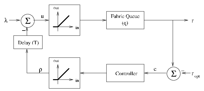
is the total arrival rate for traffic destined for the OUT queue . A total portion, , of the arriving traffic is dropped at the IN droppers, and the surviving portion goes into the fabric queue at a rate . This traffic shares the fabric queue with other traffic destined to OUT line , and then it is delivered to OUT dropper at a rate . In the analysis we assume the fabric queue is sufficiently large, so that there are no drops due to queue overflow.
The total drop rate, , is adjusted by a controller (how is distributed among the IN droppers is not relevant for this analysis; we explain how we implement the actual drop mechanism in the next section). The purpose of the controller is to keep the fabric output rate for packets destined to at a desired level, . The desired rate can be chosen according to the current rate out of
where is a constant smaller than but close to 1. In this way the desired rate will be close to the capacity, , of fabric output line when the OUT queue is the only busy queue and utilizing the entire speed of port . Furthermore it will be reduced in proportion to the service rate of when multiple OUT queues are contending for the OUT port. The two nonlinearities in the figure simply state that the drop rate can not be negative or greater than the arrival rate . In our analysis we assume that the controller is operating in the linear region, and ignore the nonlinearities.
The delay between the output of the controller and the arrival rate models a zero-order hold at the controller output. The controller operates on time-average of the error signal taken over an interval , rather than the signal itself, and modifies its output only at intervals of . In the rest of this section we denote the time-average of a signal over the period by the discrete notation . For example the time-average of the fabric output rate is given by
When the system is in steady state, the amount of traffic, , in the fabric queue destined to does not change significantly during the interval . Therefore, we can approximate the average fabric output rate by
| (2) | |||||
For a discrete PI controller the drop rate for the next interval is calculated using the error between the average fabric output rate, , and the desired fabric output rate, ,
We can now investigate the step response of the system, setting and for , for the case of a single flow. The magnitude of the arrival rate can in general be larger than the maximum fabric output rate, i.e., . In this case the fabric output will be constant at for an initial period . During this period the fabric queue will always be non-empty and the controller can not sense the actual magnitude of the arrival rate. Therefore the controller output will increase linearly,
The fabric queue size, measured at the end of each period, will increase until the drop rate reaches and then decrease back to zero
| (3) | |||||
The duration of this initial period, , and the maximum queue size can easily be calculated from this quadratic equation setting . To find the behavior of the system for we use a new time axis, , with an initial condition for the accumulator memory
where
Equations (2) and () describe a closed-loop control system. We show in the appendix that the two poles of this system are at
It follows that we have the stability condition given by the proposition below.
Proposition 1.
The closed-loop system described by (2) and () is stable iff
| (5) |
Proof.
If then , and both poles are inside the unit circle iff
which yields
On the other hand if then , and both poles are inside the unit circle iff
which yields
Combining the two cases gives the condition for stability. ∎
In the appendix we solve the system with the stability condition (5, and show that the controller output is given by
| (6) |
where
and
is the difference between the arrival and the desired rates. We observe that after the initial linear increase, the drop rate approaches exponentially to the difference between the arrival and the desired rates. Furthermore, since the absolute value of the negative pole is relatively larger for , the system will show more oscillatory behavior in this case compared to the case.
Multiple flows
When there are multiple flows, the analysis for the initial period needs to be updated. Let be the total rate of the traffic that does not belong to flow but destined to port . If the step size for flow is such that then for an initial period the average fabric output rate for flow is approximately
Since is not constant anymore, the previous results for the initial period do not apply in general. However, once the transient is over and and are adjusted so that , the approximation (2) holds, and the results for the single-flow case can be used replacing by a new initial condition. We defer a detailed analysis of the initial transient period for the multi-flow case to a future study. However, in two cases, when or is negligible compared to the other, the results for the single-flow case can be used with some changes. If , then and we can approximate the multiple-flow case by the single-flow case. On the other hand, if then we can assume that is constant since the effect of the new traffic, will be negligible. Therefore
with during the initial period . In this case is defined by
For the drop rate can be calculated by replacing (2) with
The response for is still given by (6) but with a new initial condition replacing .
Quantized PI - the Gear Box algorithm
A practical implementation of the discrete-time PI control described above requires a few modifications to the control loop. The first modification is related to how the bytes will actually be dropped at the desired drop rate calculated by the controller. The drop rate has to be divided fairly among the IN droppers. Furthermore it is well-known that dropping consecutive packets may result in poor performance in the affected flows. Therefore it is desirable to spread the drop rate to an interval and to introduce some randomness into the drop process. For these reasons we introduce a packet drop probability, , which is updated at intervals of according to the desired drop rate and the estimated average arrival rate,
| (7) |
Note that here we used the fabric output rate divided by the admit probability (i.e., ) as an estimate of the next average arrival rate. This is justified for the cases where the average arrival rate is a slowly varying function relative to interval and the delay
The second modification to the feedback structure is related to the constraint on the size of the feedback channel, which becomes a limiting factor on the precision of the feedback signal at high speeds. Our goal is to use only a finite number of drop probability values, and to derive a controller that will have a similar performance with the PI controller. For this purpose we expand (7) as
Using again the assumption , we can rewrite the above equation as
Now, if we define
then the update for the drop probability simply becomes
In order to use finite values of we quantize to three levels
| (8) |
Then the update for discrete probability values becomes
which can also be written as an update of admit probabilities as
If we set , then (8) can also be expressed in terms of the relative congestion as
where
and
We call the quantized mechanism with the Gear Box (GB) controller, since there are only three possible actions: increase the drop probability, decrease the drop probability, and no change. With the GB controller it is sufficient to have a 2-bit feedback signal every seconds. Furthermore the different levels of the admit probabilities are the different powers of . Therefore the calculation at the IN droppers can be implemented by storing
as a table in the memory and just updating a pointer to this table based on the feedback signal.
To increase the stability of the control loop, in our implementation of the GB algorithm, we choose the value for such that the relative congestion after a step increase or decrease in IN drop probability be equal. To find the value for that has this property, when note that when the relative congestion reaches , the drop step is increased, and the relative congestion immediately changes to a different value . More precisely, if we have:
then changes to , so
which can be rewritten as
Likewise, when reaches , the drop step is decreased and the relative congestion immediately changes to a different value . That is,
has the effect of changing to , yielding
that is
and we want to have . Hence,
which reduces to
giving finally
| (9) |
as the value for such that the relative congestion after a step increase or decrease in IN drop probability be equal.

We illustrate the behavior of the system when subject to the configuration of (9) in Figure 3, where . When the input rate increases such that the output relative congestion goes from to , the input drop probability remains at the same level, and jumps to when the output relative congestion reaches . This jump in the input drop probability has the immediate effect of causing the output relative congestion to decrease to a value . Then, if the output relative congestion increases again to , the input drop probability remains at before jumping to when the output relative congestion reaches . Now, if the input drop probability is at , and the relative congestion decreases from to , the input drop probability remains at , and jumps down to as soon as the relative congestion reaches . The decrease in the input drop probability from to immediately increases the output relative congestion to .
As shown in Figure 3, this configuration has the key advantage of providing hysteresis to the GB control, by always trying to have the relative congestion come back to , thereby providing stability against small perturbations. We will use this configuration in our simulations presented in the following.
5 Simulation Experiments
The objective of this section is to present a set of experimental results that illustrate the salient properties of FOQ. First, we describe a relatively simple experiment with three classes of traffic and constant-bit-rate (CBR) traffic, before presenting experimental results gathered for a more realistic situation where traffic consists of a large number of non-synchronized TCP sources.
5.1 FOQ and Service Guarantees
 (a) without FOQ
 (b) with FOQ
 (a) Input drop rate without FOQ
 (b) Input drop rate with FOQ
 (c) Fabric drop rate without FOQ
 (d) Fabric drop rate with FOQ
 (e) Output drop rate without FOQ
 (f) Output drop rate with FOQ
 (a) without FOQ
 (b) with FOQ
We simulate a 16x10 Gbps-port switch with a MB shared memory fabric having external speedup , 2 MB drop-tail OUT queues per flow, and no ingress queues. The FOQ-GB mechanism has a sampling rate ms and feedback thresholds , . We run each simulation for ms.
The offered load is composed of three flows sending at constant rates starting at : flow 0: Gbps, flow 1 and 2: Gbps each, all ingressing on separate ports and exiting the same port. Given that the total offered load is Gbps, the OUT port has a potential % overload. The required guarantee for flow 0 is Premium service ( Gbps rate guarantee), and minimum rate guarantees of Gbps and Gbps are required for flows 1 and 2 respectively. Flow 0 is assigned to Fabric queue 0 at high priority, and flows 2 and 3 to Fabric queue 1 at lower priority. At the OUT scheduler, each flow is assigned a separate queue. Queue 0 is scheduled at high priority, whereas queues 2 and 3 are scheduled at lower priority in a Weigted Fair Queuing discipline between them with weights, corresponding to the required rate guarantees.
In Figure 4 we plot the evolution in time of the service rate for the three flows, without and with FOQ respectively. In Figure 5 we show the dynamics of drop rate for the same scenarios. In all plots, each datapoint corresponds to an average over a sliding window of size 1 ms. Flow 0 is serviced at its arrival rate in both cases, due to its high priority assignment in the fabric and OUT scheduler. But the rate received by flow 1 in the non-FOQ case, Gbps (Figure 4(a)), is below its requirement. This is due to the drop in the fabric queue 1 (Figure 5(c)) without discrimination between flows 1 and 2. When using FOQ (Figure 4(b)), flow 1 receives Gbps and flow 2 Gbps, thus both achieving their minimum rate guarantees. This is explained by the FOQ action reflected in Figure 5(b) where we see an increase of input drop for flows 1 and 2 as a reaction to output congestion. As a consequence, the fabric drop is zero almost all the time in the FOQ case, in contrast with the high drop rate in the base case. The spike in fabric drop is due to the transient state where ingress drop is increasing but not yet sufficient for eliminating fabric congestion. With FOQ, fabric drop occurs only at bursts with high rate and long duration. It can be mitigated by larger fabric memory or higher frequency of feedback. Also note that flow 0 is not affected even during the FOQ transient due to its assignment to the high priority fabric queue.
In Figure 6 we show the dynamics of packet transit delay through the whole switch. While flow 0 receives minimum delay in both cases due to its high priority assignment, flows 1 and 2 experience delays that are proportional to their respective service rates (their OUT queues are close to full in the steady state due to the drop-tail queue management).
5.2 FOQ Dynamics with TCP Traffic
Next, we examine the interaction of FOQ-GB with TCP traffic. To that effect, we run a simulation where 4,500 TCP sources send traffic through a switch. In this experiment, we only consider one class of traffic. Four subnets containing 1,000 TCP sources each and one subnet containing 500 TCP sources are connected to the switch by five independent 1 Gbps links. All sources send traffic to the same destination subnet, which is also connected to the switch by a 1 Gbps link, with a one-way propagation delay of 20 ms. We have the number of active TCP flows increase over time as follows. Each source in the first subnet starts sending traffic between s and s, according to a uniform random variable. Then, each source in the second subnet starts sending traffic between s and s. Subsequently, every two seconds, sources in an additional subnet start transmitting. Hence, we have no overload between s and s, a potential 2:1 overload in the fabric between s and s, a 3:1 overload between s and s, a 4:1 overload between s and s, and a 5:1 overload then on. There is a potential bottleneck at the output port of the switch governing the 1 Gbps link to the destination subnet after s. All TCP sources send 1,040-byte packets.
 (a) Input drops
 (b) Fabric queue length
The FOQ parameters, are chosen as in the previous experiment, i.e., , and . The fabric queue has now a size of 500 KB and the output queue has a size of 400 KB. The output queue runs RED, with , KB, KB, a sampling time of 1 ms, and a weight . We compare the performance of the switch with and without FOQ.
We first observe in Figure 7(b), where each datapoint represents a moving average over a sliding window of size 50 ms, that, regardless of the potential overload, FOQ consistently manages to maintain the fabric backlog extremely close to zero, by dropping packets at the input links. As illustrated in Figure 7(a), input drops increase with the overload. Conversely, without FOQ, and therefore in the absence of input drops, the fabric buffer is filling up with the number of active TCP sources, and is eventually completely full once all sources have started transmitting. Ultimately, as illustrated in Figure 8(a), traffic is dropped in the fabric. There are no fabric drops when FOQ is used.
 (a) Fabric losses
 (b) Output losses
Last, we observe in Figure 8(b) that the output loss rate is limited by % when FOQ is disabled. On the other hand, FOQ maintains the egress relative congestion close to , as shown in Figure 9(a), and consequently, the output loss rate remains close to 9.8%. When the loss rates become roughly constant, the output queue length, represented in Figure 9(b), also becomes constant, by virtue of a stable RED control [7].
 (a) Egress relative congestion
 (b) Output queue
As a conclusion to this second experiment, we have shown that FOQ’s objectives of preventing fabric drops and regulating the traffic that arrives at the output link were met in the case of an experiment with a large number of TCP sources. The results were even more positive than those obtained with constant-rate sources, as FOQ does not exhibit transient behaviors in this scenario. This can be justified by the fact that FOQ feedback is run at a much higher frequency (every ms) than the TCP congestion control algorithms, which are run with an approximately 40-ms delay here.
6 Discussion and Conclusions
In this paper we presented the Feedback Output Queuing architecture for packet switching that provides support for service guarantees when the switching speed is limited by the memory read and write speeds. Using a fast switching fabric in this case leads to a build-up in fabric buffers and eventually either to buffer overflow and packet discarding or to unbounded delays at the fabric inputs due to backpressure. The FOQ architecture solves this problem by triggering packet discard only from flows that exceed their allocated bandwidth, and therefore limiting the build-up and delay at the fabric buffers. In the worst case the arrival rate will be , the total input capacity of the fabric. For the PI controller the maximum fabric queue size and the maximum delay in the fabric can be calculated from (3) by inserting . Any delay value above this number can be deterministically guaranteed to a flow by using a proper scheduler (e.g. WFQ-based) at the output queues after the fabric.
An alternative approach to solve the same problem is to use VOQ at fabric inputs. Recent studies show that VOQ can also provide deterministic delay bounds [21]. This is however at the expense of computational complexity. VOQ algorithms require computations per packet slot to determine which packets will be sent to their destinations. This high computational complexity makes the VOQ approach less feasible for high bit-rate switches. In contrast, the FOQ requires a total of computations per packet slot and computations per feedback interval, where is the number of supported classes. Since the feedback interval is much larger than a packet slot, computations for the feedback are actually negligible. Furthermore, the computations are distributed to the inputs and outputs, so that each input and output performs computations. In other words, FOQ’s computational complexity is much lower than VOQ, the current state of the art.
We applied discrete feedback control theory to derive a stable configuration for FOQ. Through analysis and simulations we showed that a quantized version of a PI controller named “Gear-Box control” is stable, responds quickly to traffic bursts and provides highly accurate QoS guarantees.
We believe that this work has sparked many venues for future research. There is a range of control algorithms to be investigated besides those presented here. The interaction between the TCP congestion control algorithm and FOQ (and RED queue management) is an interesing control problem. The FOQ architecture can be extended with a set of input queues in order to provide zero loss for a wider range of bursty traffic, given a limited fabric memory size.
Acknowledgments
The authors would like to thank Eric Haversat, Tom Holtey and Franco Travostino of Nortel Networks for many useful discussions.
References
- [1] T. Anderson, S. Owicki, J. Saxe, and C. Thacker. High speed switch scheduling for local area networks. ACM Transactions on Computer Systems, 11(4):319–352, November 1993.
- [2] W. Augustyn, G. Heron, V. Kompella, M. Lassere, P. Menezes, H. Ould-Brahim, and T. Senevirathne. Requirements for Virtual Private LAN Services (VPLS). IETF draft, draft-ietf-l2vpn-vpls-requirements-00.txt, October 2002.
- [3] S. Blake, D. Black, M. Carlson, E. Davies, Z. Wang, and W. Weiss. An architecture for differentiated services. IETF RFC 2475, December 1998.
- [4] M. Carugi, D. McDysan, L. Fang, F. Johansson, A. Nagarajan, J. Sumimoto, and R. Wilder. Service requirements for layer 3 provider provisioned virtual private networks. IETF draft, draft-ietf-ppvpn-requirements-04.txt, March 2002.
- [5] S.-T. Chuang, A. Goel, N. McKeown, and B. Prabhakar. Matching output queueing with a combined input-output queued switch. In Proceedings of IEEE INFOCOM ’99, volume 3, pages 1169–1178, New York, NY, March 1999.
- [6] B. Davie, A. Charny, J. Bennett, K. Benson, J.-Y. Le Boudec, W. Courtney, S. Davari, V. Firoiu, and D. Stiliadis. An expedited forwarding PHB. IETF RFC 3246, March 2002.
- [7] V. Firoiu and M. Borden. A study of active queue management for congestion control. In Proceedings of IEEE INFOCOM’00, volume 3, pages 1435–1444, Tel-Aviv, Israel, April 2000.
- [8] V. Firoiu, X. Zhang, and E. Gündüzhan. Feedback output queueing: a novel architecture for efficient switching systems. In Proceedings of Hot Interconnects X, Stanford, CA, August 2002.
- [9] S. Floyd and V. Jacobson. Random early detection for congestion avoidance. IEEE/ACM Transactions on Networking, 1(4):397–413, July 1993.
- [10] G. Franklin, J. Powell, and M. Workman. Digital control of dynamic systems. Addison-Wesley, Menlo Park, CA, 3rd edition, 1998.
- [11] B. Gleeson, A. Lin, J. Heinanen, G. Armitage, and A. Malis. A framework for IP based virtual private networks. IETF RFC 2764, February 2000.
- [12] D. Goderis, S. Van Den Bosch, Y. T’joens, O. Poupel, C. Jacquenet, G. Memenios, G. Pavlou, R. Egan, D. Griffin, P. Georgatsos L. Georgiadis, and P. Van Heuven. Service level specification semantics and parameters. IETF draft, draft-tequila-sls-02.txt, February 2002.
- [13] R. Guérin and V. Pla. Aggregation and conformance in differentiated service networks: A case study. ACM Computer Communication Review, 31(1):21–32, January 2001.
- [14] J. Heinanen, F. Baker, W. Weiss, and J. Wroclawski. Assured forwarding PHB group. IETF RFC 2597, June 1999.
- [15] V. Jacobson. Congestion avoidance and control. In Proceedings of ACM SIGCOMM’88, pages 314–329, Stanford, CA, August 1988.
- [16] K. Kar, T.V. Lakshman, D. Stiliadis, and L. Tassiulas. Reduced complexity input buffered switches. In Proceedings of Hot Interconnects VIII, Stanford, CA, August 2000.
- [17] S. McCreary and K. Claffy. Trends in Wide Area IP Traffic Patterns. CAIDA, May 2000.
- [18] N. McKeown and T. Anderson. A quantitative comparison of iterative scheduling algorithms for input-queued switches. Computer Networks and ISDN Systems, 30(24):2309–2326, December 1998.
- [19] C. Minkenberg and T. Engbersen. A combined input and output queued packet-switched system based on Prizma switch-on-a-chip technology. IEEE Communications Magazine, 38(12):70–77, December 2000.
- [20] G. Nong and M. Hamdi. On the provisioning of Quality of Service guarantees for input queued switches. IEEE Communications Magazine, 38(12):62–69, December 2000.
- [21] G. Nong and M. Hamdi. Providing QoS guarantees for unicast/multicast traffic with fixed and variable-length packets in multiple input-queued switches. In Proceedings of IEEE ISCC’01, pages 166–171, 2001.
- [22] J. Padhye, V. Firoiu, D. Towsley, and J. Kurose. Modeling TCP Reno Performance: A Simple Model and Its Empirical Validation. IEEE/ACM Transactions on Networking, 8(2):133–145, April 2000.
- [23] E. Rosen, C. Filsfils, G. Heron, A. Malis, L. Martini, and S. Vogelsang. An architecture for L2VPNs. IETF draft, draft-ietf-ppvpn-l2vpn-00.txt, July 2001.
- [24] W. Stevens. TCP slow start, congestion avoidance, fast retransmit, and fast recovery algorithms. IETF RFC 2001, January 1997.
- [25] Y. Xu and R. Guerin. Individual QoS versus aggregate QoS: A loss performance study. In Proceedings of IEEE INFOCOM ’02, volume 3, pages 1170 – 1179, New York, NY, June 2002.
Appendix
In this appendix we give a detailed derivation of some of the equations.
Taking the -transforms of (2) and (), we get
| (10) | |||||
and
| (11) |
Transfer functions of this system between the output rate, , and the two inputs and initial state, , , and , are given by
and
Let and be two roots of the system characteristic equation, i.e.
Then without loss of generality
We showed in Proposition 1 that the system is stable if
We next find the solution for the drop rate assuming this stability condition is satisfied. For step inputs and initial condition, , , , and defining as the difference between the arrival and the desired rates, we have from (10) and (11):
This can be written as a partial fraction expansion as
where
and
which can be solved easily. Finally recall that this system was obtained initially by defining a new time axis for . Therefore after taking the inverse -transform we combine the result with case to get