Algebraic Curves in Parallel Coordinates
– Avoiding the “Over-Plotting” Problem
Abstract
ntil now the representation (i.e. plotting) of curve in Parallel Coordinates is constructed from the point line duality. The result is a “line-curve” which is seen as the envelope of it’s tangents. Usually this gives an unclear image and is at the heart of the “over-plotting” problem; a barrier in the effective use of Parallel Coordinates. This problem is overcome by a transformation which provides directly the “point-curve” representation of a curve. Earlier this was applied to conics and their generalizations. Here the representation, also called dual, is extended to all planar algebraic curves. Specifically, it is shown that the dual of an algebraic curve of degree is an algebraic of degree at most in the absence of singular points. The result that conics map into conics follows as an easy special case. An algorithm, based on algebraic geometry using resultants and homogeneous polynomials, is obtained which constructs the dual image of the curve. This approach has potential generalizations to multi-dimensional algebraic surfaces and their approximation. The “trade-off” price then for obtaining planar representation of multidimensional algebraic curves and hyper-surfaces is the higher degree of the image’s boundary which is also an algebraic curve in -coords.
keywords: Visualization, Parallel Coordinates, Algebraic Dual Curves, Approximations of Algebraic Curves, Surfaces.
AMS : 76M27
ACM : F.2.1, I.1.1
1 Parallel Coordinates
ver the years a methodology has been developed which
enables the visualization and recognition of multidimensional
objects without loss of information. It provides insight
into multivariate (equivalently multidimensional) problems and
lead to several applications. The approach of Parallel Coordinates
(abbr. -coords) [5] is in the spirit of
Descartes, based on a coordinate system but differing in an
important way as shown in Fig 1. On the Euclidean
plane (more precisely on the projective plane
) with -Cartesian coordinates, copies of a
real line, labelled ,
are placed equidistant and perpendicular to the -axis with
and being coincident. These lines, which have
the same orientation as the -axis, are the axes of the Parallel Coordinate system for the -dimensional Euclidean
space . A point is represented by the polygonal line having
vertices at the values on the -axes. In this way a
one-to-one correspondence is established between a points in
and planar polygonal lines with vertices on the
parallel axes. The polygonal line contains the complete lines and not just the segments between adjacent axes.

The restriction to provides that not only is a point represented by a line, but that a line is represented by a point. The points on a line are represented by a collection of lines intersect at a single point as can be seen in Fig. 2; i.e. a “pencil” of lines in the language of Projective Geometry. A fundamental duality is induced which is the cornerstone of deeper results in -coords. The multidimensional generalizations for the representation of linear -flats in (i.e. planes of dimension ), in terms of indexed points have been obtained. The proper setting for dualities is the projective rather than the Euclidean plane . A review of the mathematical foundations is available in [6].
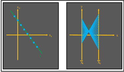

For non-linear, especially non-convex, objects the representation
is naturally more complex. In a point-curve, a curve
considered as collection of points, is transformed into a line-curve; a curve prescribed by it’s tangent lines as in Fig.
3. The line-curve’s envelope, a point-curve, is the
curve’s image in -coords. In many cases this yields an image
that is difficult to discern. This point requires elaboration in
order to motivate and understand some of the development presented
here. As posed, the construction of a curve’s image involves the
sequence of operations:
Unlike the example shown in Fig. 3, where the line-curve’s image is clear, the plethora of overlapping lines obscures parts of the resulting curve-line. This is a manifestation of what is sometimes called “over-plotting” problem in -coords; the abundance of “ink” in the picture covers many underlying patterns. Simply our eyes are not capable of “extracting” the envelope of lots of overlapping lines. There are also computational difficulties involved in the direct computation of the image curve’s envelope. In a way this is the “heart” of the “over-plotting” problem considered as a barrier in the effective use of -coords. This problem can be overcome by skipping the intermediate step and go to an equivalent
transformation which provides directly a clear image. as shown in Fig. 5.


This point-to-point mapping (Inselberg Transformation [5] ) preserves the curve’s continuity properties. The idea is to use the part of the duality and map the tangents of the curve into points as illustrated in Fig. 5. Therefore, a curve is represented by a point-curve (the “dual curve”) in the -coords plane. For a point-curve, , defined implicitly by
| (1) |
the coordinates of the point-curve image (i.e. dual) are given by
| (2) |
It was shown by B. Dimsdale [1] and generalized
in [5], using this transformation that conics
are mapped into conics in 6 different ways [1].
Here we develop the extension of the dual image for the family of
general algebraic curves. This family of curves is highly
significant in many implementations and applications, since these
curves can easily and uniquely be reconstructed from a finite
collection of their points (for instance using simple
interpolation methods [7],
[13]). Approximations of such curves can
simply be obtained using similar methods.
As will be seen, the dual of an algebraic curve in general has
degree higher than the original curve. There are some
fringe-benefits, illustrated later, where “special-points” such
as self-intersections or inflection-points which are conveniently
transformed. But we do not want to get ahead of ourselves. The key
reason for this effort is to pave the way for the representation
of algebraic curves and more general hyper-surfaces, as well as
their approximations, in terms of planar regions without
losing information. To pursue this goal then we need firstly to
study the image of curves starting with general algebraic curves.
2 Transforms of Algebraic Curves
2.1 The Idea Leading to the Algorithm
n order to
represent non-linear relations in -coords it is essential to
extend the representational results first to algebraic curves;
those described by either, explicitly or implicitly by irreducible
polynomials of arbitrary degree. The direct application of eq.
(2) turns out to be difficult even for degree 3. There
is a splendid way to solve this problem using some ideas and tools
from Algebraic Geometry. These involve properties of homogeneous
polynomials and Resultant which are explained during the
development of the method. For extensive treatments the reader is
referred to [8], [10],
[11] and [12].
Starting with an algebraic curve defined by an
irreducible polynomial in its image
in -coords is sought. A number of preparatory steps smooth the
way for the easier application of the transformations in eq.
(2). First the curve is
“raised” to a surface embedded in the projective space
and only then the corresponding mapping into
-coords is applied.
-
There exists a one-to-one correspondence (preserving the reducibility of polynomials) between any polynomial of degree and a homogenous polynomial in the projective plane , which is obtained by using homogeneous coordinates. Specifically,
- •
replace by for ,
- •
multiply the whole polynomial by and simplify.
These multiplications are, of course, allowable for . The result is a homogeneous polynomial (which is also irreducible if is) with each term having degree . To wit,
(3) which describes a surface in where the original polynomial curve is embedded as:
(4) 
Figure 6: Cone generated by embedding the curve in . - •
-
The Gradient of is found and denoted by :
The three derivatives provide the direction numbers of the normal to the tangent plane at the point . It is a fundamental property of homogeneous polynomials that
(5) where is the degree of . In our case and hence the equation of the tangent planes is
(6) Since the tangent plane at any point of the surface goes through the origin it is clear that the surface is a cone with apex at the origin as shown in Fig. 6.
-
Substituting for from eq. (6) in
(7) provides the intersection of the tangent plane with the cone which is a whole line as shown in Fig. 7. Each one of these lines, of course, goes through the origin and therefore it can be described by any one other of its points and in particular by . Simplifying the homogeneous coordinates by,
results in
(8) By the way, this is also a homogeneous polynomial in the five variables appearing in its argument.

Figure 7: The intersection of the cone with any of it’s tangent planes is a whole line. Along such a line the direction numbers are constant and unique. It is helpful to understand the underlying geometry. Eq. (8) can be considered as specifying a family of lines through the origin and through each point along the curve given by eq. (4). Alternatively, the cone can be considered as being generated by a line, the generating line – see Fig. 8, pivoted at the origin and moving continuously along each point of the curve described by eq. (4). On each one of these lines the direction numbers are unique and constant as shown in Fig. 8; i.e. there is a one-to-one correspondence:
Eq. (7), and hence it’s rephrasing eq. (8), contains two equivalent descriptions of the cone, i.e. in terms of the coordinates and also the direction numbers . Hence one can be eliminated and as it turns out it is best to eliminate the something which is very conveniently done by means of the Resultant. The resultant of two homogenous polynomials
and
is the polynomial obtained from the determinant of their coefficients matrix:
where the empty spaces are filled by zeros. There are lines of and lines of . When and are both irreducible so is their resultant. Due to the homogeneity of and ,
Let us rewrite eq. (8) as
(9) Appealing again to the homogeneity of to obtain the relation
which has already been mentioned earlier. Therefore
and from the property of the resultant of homogeneous polynomials mentioned above
Altogether then
(10) has finite degree since and are polynomials. It was shown that
so not only their zero sets agree, which ensures that they are equivalent polynomials, but they also agree at an infinite number of points. Hence, provides the description of the cone in terms of the direction numbers and is also a homogeneous polynomial. The degree of is . This and the structure of the resultant with the four triangular zero portions results in being a polynomial of degree at most .

Figure 8: This shows the generating line of the cone (which is found from the intersection of the tangent planes with the cone) together with the gradient vector. -
Since we are interested in the solutions of the multiplier in powers of of , if there is one, can be safely neglected due to the homogeneity.
-
Only in this, the final step, the transformation of the curve from the -plane to the -plane with parallel coordinates is performed. It is done using equations (2) rewritten, in view of eq. (6) as
(11) It is important to notice that both this and eq. (10) involve only the derivatives . Let , so that , and . Substitution provides the transform of the original curve :
when . In the previous step it was pointed out that this polynomial has degree at most , the actual degree obtained depends on the presence of singular points in the original algebraic curve .
2.2 Algorithm
ere the process involved is
presented compactly as an algorithm [3] whose input
is an algebraic curve and the output
is the polynomial which describes , the curve’s
image in -coords. To emphasize, the algorithm applies to
implicit or explicit polynomials of any degree and curves with or
without singular points. The formal description of the algorithm
is followed by examples which clarify the various stages and their
nuances.
For a given irreducible polynomial equation (otherwise apply the
algorithm for each of it’s component separately)
.
- 1.
Convert to homogeneous coordinates to obtain the transformation of , a homogenous polynomial .
- 2.
Substitute
, and
. - 3.
Find the resultant of the two derivatives and .
- 4.
Cancel the multiplier in a power of of the resultant and denote the result by .
- 5.
The output is obtained by the substitution
, , in .
3 Examples of Algebraic Curves and their Transforms
3.1 Conic Transforms
he algorithm is
illustrated with some examples starting with the conics.
Applying the algorithm in the sequence given above:
-
The homogeneous polynomial obtained from by using homogeneous coordinates is
-
Substituting
yields
where , for .
-
Calculate the two derivatives of and their resultant:
-
Retain the resultants component which is multiplied by a power of and let
-
The dual of is then given in matrix form by
where the individual are :
The result is illustrated for the ellipse in fig 9 and can also be contrasted to the earlier ways for obtaining the transformation

3.2 Algebraic Curves of Degree Higher than Two
ext the algorithm is applied to the algebraic curve of 3rd degree


-
The homogeneous polynomial obtained from by using homogeneous coordinates is
-
Substituting
yields
where the , for .
-
Calculate the resultant of the two derivatives of :
where is polynomial of degree 6.
-
Discarding the resultant’s factor i.e. let
-
Finally, substituting
results in the 6th-degree curve :
The source and image curve are shown in Fig. 10.
In this case and the maximum degree
is attained. Notice that this covers as special cases :
– the point line duality where points
(with ) are mapped into lines (with ) and
vice-versa, and
– the conics with .
The next two examples show that the image curve may have degree
less than . Apparently the maximal degree is attained by
the image curve in the absence of singularities in the function or
it’s derivatives. The full conditions relating the image’s degree
to less then the maximal are not known at this stage. Two such
examples are shown in the subsequent figures, Fig. 11
and Fig. 12.

4 Conclusions
onsider the class of hyper-surfaces in which are the envelopes of their tangent hyper-planes. As mentioned earlier [6] hyper-planes can be represented in -coords by indexed points. Hence for a hyper-surface each point maps into indexed planar points. From this it follows that the hyper-surface can be mapped (i.e. represented) by indexed planar regions composed of these points. Restricted classes of hyper-surfaces have been represented in this way and it turns out that the reveal non-trivial properties of the corresponding hyper-surface . It has already been proved that for any dimension Quadrics (algebraic surfaces of degree 2) are mapped into planar regions whose boundaries are conics [4]. This also includes non-convex surfaces like the “saddle”. There are strong evidence supporting the conjecture that algebraic surfaces in general map into planar regions bounded by algebraic curves. This, besides their significance on their own right, is one of the reasons for studying the representation of algebraic curves. In [2] families of approximate planes and flats are beautifully and usefully represented in -coords. Our results cast the foundations not only for the representation of hyper-surfaces in the class , but also their approximations in terms of planar curved regions.
Acknowledgments
he author would like to thank to Prof. Alfred Inselberg for his grate help and his kindly support. The author acknowledge and is grateful for the use of the symbolic manipulation program Singular developed by the Algebraic Geometry Group, Department of Mathematics, University of Kaiserslautern, Germnay.
References
- [1] B. Dimsdale, “Conic transformations and projectivities”, IBM Los Angeles Scientific Center, 1984, Rep. G320-2753.
- [2] A. Inselberg and T. Matskewich, “Approximated planes in parallel coordinates”, Vanderbilt University Press, Paul Sabloniere Pierre-Jean Laurent and Larry L. Shumaker (eds.), Eds., 2000, pp. 257–267.
- [3] Z. Izhakian, “An algorithm for computing a polynomial’s dual curve in parallel coordinates”, M.sc thesis, Department of Computer Science, University of Tel Aviv, 2001.
- [4] Z. Izhakian, “New Visualization of Surfaces in Parallel Coordinates - Eliminating Ambiguity and Some Over-Plotting”, Journal of WSCG - FULL Papers Vol.1-3, No.12, ISSN 1213-6972, 2004, pp 183-191.
- [5] A. Inselberg, “The plane with parallel coordinates”, The Visual Computer, vol. 1, no. 2, pp. 69–92, 1985.
- [6] A. Inselberg, “Don’t panic … do it in parallel!”, Computational Statistics, vol. 14, pp. 53–77, 1999.
- [7] R. L. Burden and J. D. Faires, “Numerical analysis”, 4th ed, PWS-Kent, Boston, MA, 1989.
- [8] D. Cox, J. Little, and D. O’Shea, “Ideals, Varieties, and Algorithms”, Springer, New York, second ed. edition, 1997.
- [9] G. b. Folland, “Real analysis: modern techniques and their applications”, Wiley, New York, second ed. 1999.
- [10] J. Harris, “Algebraic geometry”, A first course, Springer-Verlag, New York, 1992.
- [11] W. Hodge and D. Pedoe, “Methods of algebraic geometry”, Vol. II. Cambridge: Cambridge Univ. Press, 1952.
- [12] R. J. Walker, “Algebraic Curves”, Springer-Verlag, New York, 1978.
- [13] G. Walter, “Numerical analysis : an introduction”, Birhauser, Boston, 1997.
*ex1, ex2