A Novel Evolutionary Formulation of the Maximum Independent Set Problem
Abstract
We introduce a novel evolutionary formulation of the problem of finding a maximum independent set of a graph. The new formulation is based on the relationship that exists between a graph’s independence number and its acyclic orientations. It views such orientations as individuals and evolves them with the aid of evolutionary operators that are very heavily based on the structure of the graph and its acyclic orientations. The resulting heuristic has been tested on some of the Second DIMACS Implementation Challenge benchmark graphs, and has been found to be competitive when compared to several of the other heuristics that have also been tested on those graphs.
Keywords: Maximum independent sets, evolutionary algorithms, genetic algorithms.
1 Introduction
Let be an undirected graph of node set and edge set such that and . An independent set (or stable set) of is a subset of containing no neighbors (nodes that are connected by an edge in ). The set is a node cover of , that is, a set of nodes that includes at least one of the two end nodes of every edge. We call every subset of whose nodes are all neighbors of one another in a clique. The complement of is an undirected graph of node set in which two nodes are neighbors if and only if they are not neighbors in . Clearly, is an independent set of if and only if it is a clique of .
We are concerned in this paper with the problem of finding a maximum independent set in , that is, an independent set of maximum size. Equivalently, this problem can be viewed as asking for a minimum node cover in or a maximum clique in . Finding independent sets (or any of the other equivalent structures) of extremal size has several important applications. We refer the reader to the volume that resulted from the Second DIMACS Implementation Challenge [38] for various examples of application areas, and to [25] for further examples from coding theory.
The problem of finding a maximum independent set in is NP-hard (it is NP-complete when formulated as a decision problem [39, 26]), and remains NP-hard even if we settle for solving it approximately within of the optimum for any [3, 4, 12]. That is, if is the size of a maximum independent set of (the independence number of ), then finding an independent set of size at least is NP-hard.
Our formulation of the maximum independent set problem is based on the notion of an acyclic orientation of , i.e., an assignment of directions to the edges of that leads to no directed cycles. Let denote the set of all the acyclic orientations of . For , let be the set of all chain decompositions of the nodes of according to , that is, each member of is a partition of into sets that correspond to chains (directed paths) according to . For , let denote the number of chains in . Our point of departure is the following equality, which relates the independence number of to its acyclic orientations [23]:
| (1) |
By (1), is the number of chains in the chain decomposition of into the fewest possible chains, according to the acyclic orientation of for which that number is greatest. This result is a refinement of Dilworth’s theorem [24] and is illustrated in Figure 1, where two acyclic orientations of the same graph are shown alongside the corresponding minimum chain decompositions. In the figure, the bottommost acyclic orientation is the one whose minimum chain decomposition is greatest, thence for the graph in question.

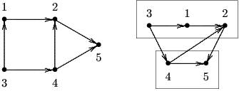
As we see it, the greatest significance of (1) is that it spells out how the set can be regarded as a set of individuals, the fittest of which yields the independence number of .11 1 A relation dual to the one in (1) indicates how to express the chromatic number of (cf. [14]) in terms of its acyclic orientations [23]. The use of that other relation in an evolutionary approach to find the graph’s chromatic number has been developed by one of us and collaborators [11]. Viewing the maximum independent set problem from this perspective is based on taking as the measure of fitness for individual and on searching for an individual of maximum fitness.22 2 is a set of vast dimensions. For example, the number of distinct acyclic orientations of is if is a tree, if it is a complete graph (all nodes connected to all others), and if it is a ring. In general, and remarkably, the number of members of is given by the absolute value of the chromatic polynomial of (cf. [14]) applied to the negative unit [48].
We develop this evolutionary approach in the remainder of the paper, starting in Section 2, where the details of the new formulation are introduced, including how to compute an individual’s fitness and the evolutionary operators of crossover and mutation for . We then continue in Section 3 with a description of the graphs to be used in our experiments, whose results are reported in Section 4. Conclusions are given in Section 5.
2 The formulation
The key to a better understanding of how to use (1) is that , the purported measure of fitness for individual , is in fact the size of an independent set that can be unequivocally obtained from orientation . In order to see this, we associate a directed graph, call it , with oriented by . This directed graph has nodes: two distinguished nodes, called and , and two nodes, called and , for each node . For every , has an edge directed from to and another from to . For every that is directed by from to , in an edge exists from to . Node is therefore a source (a node with no edges directed inward) and node a sink (a node with no edges directed outward). An illustration of this construction is given in Figure 2, where the directed graphs corresponding to the two acyclic orientations of Figure 1 are shown.


We now regard as a flow network whose edges either have unit capacity (those leaving or arriving at ) or infinite capacity (all others), and consider the maximum flow from to , whose value we assume to be . This flow is necessarily integral, as illustrated in Figure 2, where solid lines have been used to draw edges carrying unit flow and dashed lines those carrying zero flow. It also establishes a chain decomposition of according to into chains. Take, for example, the topmost network of Figure 2, where . If we only follow edges carrying unit flow, then we can easily trace the single chain , , , . For the bottommost network, and we get the two chains , and . These, readily, are the minimum chain decompositions according to the two acyclic orientations.
What is left to note is that only edges leaving or arriving at can be saturated by the maximum flow, so the corresponding minimum cut is necessarily given by a group of such edges. In Figure 2, the minimum cut in each network is indicated by boxes enclosing the nodes other than or that are involved in the cut. Such nodes do necessarily constitute a minimum node cover of the edges that do not involve or in , and consequently induce a node cover in as well ( for the topmost network, for the other) with a corresponding independent set ( and , respectively).
In general, then, we have the following [2]. If is the value of the maximum flow from to in , then is the number of chains in the minimum chain decomposition of according to and is the size of a node cover in . Consequently, is also the size of an independent set in . In order to determine the actual nodes that constitute this independent set, it suffices to look at the minimum cut in and at the node cover it induces on the edges of that do not touch or . This node cover corresponds to a node cover in as well, whose complement with respect to is then the desired independent set.
We now turn to the three key elements of our formulation, namely how to assess an individual’s fitness and how crossover and mutation operate. We have designed these elements in such a way that they can be used directly in most standard templates of fitness-maximization genetic algorithms [30, 45]. What is novel in our formulation is the adoption of as the search space out of which populations are formed. Not only do the acyclic orientations of relate cleanly, as we have discussed, to the independent sets of , but also they allow for evolutionary operators that are simple and yet effective in several aspects of the evolutionary search. We will come to them shortly.
Fitness evaluation
For , let denote the fitness to be maximized over while searching for a maximum independent set of . By (1), we have
| (2) |
that is, the fitness of individual is the number of chains in the minimum chain decomposition according to that orientation.
It follows from our preceding discussion that can be assessed along the following steps:
- 1.
Construct the flow network .
- 2.
Compute the value of the maximum flow from to in .
- 3.
Let .
We note, with regard to Step 2, that only the value of the maximum flow is needed for fitness evaluation, not the actual flow. In other words, what is needed is the maximum total flow incoming to , not the particular assignment of flows to all edges. When a push-relabel method is used to compute the maximum flow, it is a simple matter to separate the computation into two phases [29]: the first phase computes but may leave excess flow at some nodes; the second phase corrects this by returning flow in order to eliminate excesses. Conveniently, one of the most successful implementations currently available of a maximum-flow algorithm does precisely this [22], and as such allows the computation to stop at the end of the first phase, right after has been found. What is also convenient is that, when push-relabel methods are thus implemented, at the end of the first phase the minimum cut is also known, which is useful for determining the independent set that corresponds to the best individual found during the evolutionary search, in the manner we indicated earlier in this section. We return to this in Section 4.
Crossover
The crossover of the two individuals to yield the two offspring is best described in terms of a linear representations of the individuals involved. For individual , the representation we adopt, denoted by , is the sequence , where are the nodes of . In this sequence, and for , node appears to the left of (i.e., ) if is an edge of and is oriented by from to . For example, both and are valid linear representations of the bottommost acyclic orientation of Figure 1. Clearly, represents unambiguously, though not uniquely.
Now let and . Let also such that be the crossover point. Then and , where
- •
;
- •
is the subsequence of comprising all nodes that are not in ;
- •
;
- •
is the subsequence of comprising all nodes that are not in .
Notice that the and thus determined are valid linear representations of acyclic orientations, since, by construction, both sequences contain all nodes from . Furthermore, and inherit edge orientations from and as follows:
- •
Edges joining nodes in the set to any other nodes are oriented by exactly as by .
- •
Edges joining nodes in the set exclusively are oriented by exactly as by .
- •
Edges joining nodes in the set to any other nodes are oriented by exactly as by .
- •
Edges joining nodes in the set exclusively are oriented by exactly as by .
Mutation
Like crossover, our mutation operator is defined in terms of the linear representations of individuals. We use single-locus mutation at the mutation point with . For individual , the mutation operator turns node into a source, thus yielding another acyclic orientation . That is indeed acyclic has been argued elsewhere [10]: in essence, a directed cycle through would be required for not to be acyclic, which is impossible, being a source according to .
We also refer the reader elsewhere ([11], Section 4) for an argumentation as to why this type of mutation does more for the evolutionary search than simply to allow occasional random jumps loosely intended to escape local optima. Specifically, what is shown is that, for any two acyclic orientations , there necessarily exists a finite sequence of mutations that turns into . So this operator can be regarded as providing the search space with an underlying fundamental connectedness that allows, at least in principle, every acyclic orientation to be reached regardless of where the evolutionary search is started.
3 The experimental test set
In this section we give a brief description of the benchmark graphs used in the experiments reported in Section 4. They have all been extracted from the DIMACS challenge suite [49]. That suite is structured from the perspective of finding maximum cliques, so the graph types listed next characterize .
c-fat- [34]. This graph comes from fault-diagnosis problems [13] and its set of nodes is partitioned into sets of approximately equal sizes. Edges are deployed so that every node is connected to every other node in its own set and in the two sets that are neighbors to its own (according to an arrangement of the sets into a ring).
johnson-- [34]. This graph arises in problems from coding theory. It has nodes, each node labeled with a -digit binary number having exactly ’s. Two nodes are joined by an edge if the Hamming distance between their labels (the number of digits at which they differ) is at least .
keller [41]. This graph is derived from another with nodes which arises in connection with proving Keller’s 1930 conjecture false for high dimensions. The conjecture is that a “tiling” of Euclidean -dimensional space by unit cubes necessarily contains two cubes meeting in a full -dimensional face.
hamming- [34]. This graph comes from coding-theory problems also and has nodes, each node labeled with a -digit binary number. Two nodes are connected if the Hamming distance between their labels is at least .
san__x [36]. This graph is artificially constructed on nodes to have a maximum clique whose size is determined beforehand. Its number of edges is ; x is only used to differentiate among instances.
sanr_ [36]. This is a random graph on nodes, generated by adding an edge with constant probability between any two distinct nodes [15]. It is expected to have dimensions close to those of san__x for .
brock_x [18]. This is a random graph on nodes, designed to have a maximum clique much larger than would be expected from the nodes’ degrees. The number x is used for instance differentiation.
p_hat-x [46]. This is a random graph on nodes whose density is based on two parameters. This contrasts with the usual random graphs with fixed edge probability [15], leading to node degrees that are more spread and to larger cliques also. The number x differentiates among instances.
MANN_ax [44]. This graph gives the clique formulation of the instance of the Steiner triple problem. This formulation is obtained by a conversion from the set-covering formulation of that problem [43].
Details on the graphs we used in our experiments are given in Tables 1 and 2. For each , the tables give the values of and (the number of edges in ), as well as , when known from design characteristics.
| c-fat- | |||
|---|---|---|---|
| c-fat- | |||
| c-fat- | |||
| c-fat- | |||
| c-fat- | |||
| c-fat- | |||
| c-fat- | |||
| johnson-- | |||
| johnson-- | |||
| johnson-- | |||
| johnson-- | |||
| keller | |||
| hamming- | |||
| hamming- | |||
| hamming- | |||
| hamming- | |||
| san__1 | |||
| san__2 | |||
| san__1 | |||
| san__2 | |||
| san__3 | |||
| san__1 | |||
| san__1 | |||
| san__2 | |||
| san__3 | |||
| san__1 |
| sanr_ | |||
|---|---|---|---|
| sanr_ | |||
| sanr_ | |||
| sanr_ | |||
| brock_1 | |||
| brock_2 | |||
| brock_3 | |||
| brock_4 | |||
| brock_1 | |||
| brock_2 | |||
| brock_3 | |||
| brock_4 | |||
| p_hat-1 | |||
| p_hat-2 | |||
| p_hat-3 | |||
| p_hat-1 | |||
| p_hat-2 | |||
| p_hat-3 | |||
| MANN_a9 | |||
| MANN_a27 |
4 Experimental results
Henceforth, we refer as WAO to the algorithm that results from the formulation of Section 2. This denomination is an acronym after “Widest Acyclic Orientation,” as by (1) what is sought during the evolutionary search is an acyclic orientation whose minimum chain decomposition has the most chains over .
WAO iterates for generations, each one characterized by a population of fixed size . After generating the last population, it outputs the best individual found during the entire evolutionary search. For , the th population is obtained from the st population as follows. First an elitist step is performed, resulting in the transfer of the fittest individuals from the current population to the new, with . Then WAO performs the following iteration until the new population is full: with probability , two individuals are selected from the current population and the crossover operator is applied to them, the resulting two individuals being then added to the new population; with probability , one single individual is selected from the current population and then is subjected to the mutation operator before being added to the new population.
In order to decide on an appropriate selection method, we ran several initial experiments on reasonably-sized graphs. From these experiments emerged not only the selection method of our choice but also the suite of parameters we would adopt in all further experiments (we discuss these later). The selection method we used in our experiments picks individuals proportionally to their linearly normalized fitness in the current population. For , this means that the th fittest individual—that is, such that is the th greatest—is selected with probability proportional to
| (3) |
Ties between two individuals are broken by taking the individual that was added to the current population first as the fitter one. In (3), is the factor by which the linearly normalized fitness of the fittest individual in the current population (the case) is greater than that of the least fit individual (the case); that is, , where and are those two individuals, respectively.
We present our results in comparison to those obtained by the heuristics of the DIMACS challenge [38]. This is not to say that the best results known to date are necessarily the ones obtained by those heuristics, since several new methods have appeared in the meantime for the maximum independent set problem under one of its guises (e.g., [19, 16] and their references). However, all those more recent methods invariably go back to the DIMACS challenge heuristics as references for comparison, so those heuristics serve as an indirect basis for other comparisons as well. One exception to this comparison rule we have adopted is the genetic-algorithm approach of [1], which, like WAO, employs a nontrivial crossover operator. We present next a brief description of all the eleven heuristics to which we compare WAO directly.
B&C [7]. This is a branch-and-cut method for which cutting planes are generated based on the more general technique of [6]. It starts with an integer programming formulation of the maximum clique problem, and proceeds from the initial relaxation by generating new cutting planes and incorporating them into the current linear program.
Cliqmerge [8]. This heuristic is based on a procedure that finds a maximum clique in the subgraph induced by the nodes of two cliques when they are merged together. The essence of the method is to find a maximum bipartite matching in the complement of this subgraph.
Squeeze [17]. This is a branch-and-bound algorithm for the maximum independent set problem. Its lower bounds are obtained through a reduction to the problem of minimizing a general quadratic - function.
CBH [27]. This is an interior-point approach (cf. [32]) to the determination of maximum independent sets. Following a continuous formulation of the problem, a relaxation of it is solved and the resulting solution is rounded by a heuristic based on [20, 5].
RB-clique [31]. This method uses backtracking “coordinates” as the entities on which restricted backtracking is to be applied while seeking a maximum clique. The restrictions to which the backtracking coordinates are subject are given as input.
AtA [33]. This strategy employs recurrent neural networks (cf. [9]) to find maximum cliques. The crux of the approach is an adaptive procedure for the determination of appropriate threshold parameters and initial state for the neural network.
SA&GH [35]. This is a blend of heuristics to find maximum cliques. In most cases it employs simply simulated annealing [40], but for very dense graphs the greedy heuristic of [37] is used.
XSD [36]. This is a family of heuristic methods to find maximum cliques. The methods are all related to neural-network models and include deterministic and stochastic descent approaches, with or without an intervening learning step between restarts.
B&B [44]. This is a branch-and-bound approach to the maximum independent set problem. Upper bounds are obtained through a procedure derived from edge projection, a specialization of the clique projection of [42].
XT [47]. This is a family of three variants of tabu search [28], two deterministic and one probabilistic.
OCH [1]. This is a genetic algorithm for the maximum independent set problem. Each individual is an -digit binary number, each digit indicating whether the corresponding node is in the independent set or not. The centerpiece of the method is the so-called optimized crossover, which generates one optimal offspring based on the same merging procedure of Cliqmerge and one other having a random character.
All the experiments we report on were conducted with , , , , and . As we indicated earlier, these reflect policies and values that emerged from early experiments on reasonably-sized graphs. They by no means represent optimal decisions of any sort, since the number of possible choices is, naturally, far too large.
In all experiments, we also made use of the maximum-flow code of [21], which implements the algorithm of [22], to compute the value of as explained in Section 2. As we also indicated in that section, it suffices for the maximum-flow computation to stop right after completing its first phase, since the value of the maximum flow, and hence the size of the independent set that the individual contributes, is already known at this point. We also recall that running the maximum-flow code through its first phase only is sufficient even for the best individual found during the whole evolutionary search. In this case, what we need is to enumerate the members of the independent set contributed by that individual, not simply to know its size, but this can be obtained by examining the minimum cut that is also already known as the first phase ends.
Our results are shown in Figures 3 and 4, and in Tables 3 through 8. The two figures show, for ten graphs selected from Tables 1 and 2, the evolution of the best fitness (as given by (2)) ever found for an individual as the generations elapse during the best of twenty independent runs (the one that eventually yielded the largest independent set for that graph). In other words, they show the size of the largest independent set yet identified. These ten graphs were selected because, in terms of what is shown in Figures 3 and 4, they have led the evolutionary search to behave either in a way that we found to be somewhat typical or a way that yields interesting insight. We return to this shortly.
Tables 3 through 8 show the results obtained by WAO alongside the results of the competing algorithms we outlined earlier in this section. Tables 3–5 refer to the graphs in Table 1, while Tables 6–8 refer to those in Table 2. For each graph , the tables give the value of , when known from design characteristics, and the sizes of the maximum independent sets obtained by the algorithms on , when available. The result reported for WAO on each graph is the best result found over twenty independent runs. For the other methods, the results reported are the best results they yielded, as published in [38]. The number appearing in parentheses next to “WAO” in Tables 5 and 8 is the value of that was used to obtain the results listed in the corresponding column.
The several runs of WAO were executed on a relatively wide assortment of machine architectures, so we refrain from providing detailed timing data. Also, comparing running times to those of the other methods—obtained roughly one decade ago—would be cumbersome however we tampered with the numbers seeking to compensate for the technological gap. Given these constraints, all we do is mention that each of our runs tended to complete somewhere between very few seconds and a week, depending on the graph at hand.
WAO is a competitive method, by all that can be inferred from Tables 3–8. We have in the tables used a bold typeface to indicate the instances on which WAO performed at least as well as the best performers. Several entries are thus marked, and for many that are not WAO is seen to have fallen short by a very narrow margin.
Returning to the plots in Figures 3 and 4 may highlight some of the patterns that help explain success or failure at meeting the best performers’ figures during our experiments with WAO. Of the ten graphs to which those figures refer, three correspond to cases in which WAO missed by a narrow margin (san__1, sanr_, and brock_4) and one to a case in which it missed widely (brock_4). What seems to distinguish one group from the other is that in the latter case the plot becomes flat early in the evolution, perhaps signaling an inherent hardness at escaping some particularly difficult local maximum. For the three graphs in the former group, however, and in fact for the six graphs in the figures outside either group, evolution seems to lead to fitness growth more or less steadily along a comparatively larger number of generations, even though for the san graphs it nearly stalls for a significant number of generations before it gains momentum again. In the case of san__1, particularly, it appears quite likely that a few more generations would have bridged the narrow gap between the that WAO achieved and the of its best contenders.
5 Concluding remarks
We have in this paper introduced WAO, a novel evolutionary heuristic for the maximum independent set problem. WAO is based on a view of the problem that relates independent sets to the acyclic orientations of the graph, and seeks to identify an acyclic orientation that is widest (has the decomposition into the fewest number of chains that requires the most chains) over the set of all the acyclic orientations of the graph. It incorporates no additional sophistication into the usual evolutionary-algorithm machinery, but rather into the design of the individuals’ representations and the evolutionary operators, all based on complex graph-theoretic notions.
We have found our new heuristic to perform competitively when compared to several others on the DIMACS benchmark graphs. Notwithstanding this, there certainly is room for further investigation and improvements. For example, there may exist a better set of parameters for the evolutionary search, just as there may exist a better functional dependence of and on (and perhaps also on , unlike what we adopted in our experiments). Likewise, it is also conceivable that the formulation itself may be improved by the incorporation of optimizations into the crossover or mutation operator, or even by the introduction of new operators.
Acknowledgments
The authors acknowledge partial support from CNPq, CAPES, the PRONEX initiative of Brazil’s MCT under contract 41.96.0857.00, and a FAPERJ BBP grant.

|

|

|

|

|

|

|

|

|

|
| B&C | Cliqmerge | Squeeze | CBH | ||
|---|---|---|---|---|---|
| c-fat- | |||||
| c-fat- | |||||
| c-fat- | |||||
| c-fat- | |||||
| c-fat- | |||||
| c-fat- | |||||
| c-fat- | |||||
| johnson-- | |||||
| johnson-- | |||||
| johnson-- | |||||
| johnson-- | |||||
| keller | |||||
| hamming- | |||||
| hamming- | |||||
| hamming- | |||||
| hamming- | |||||
| san__1 | |||||
| san__2 | |||||
| san__1 | |||||
| san__2 | |||||
| san__3 | |||||
| san__1 | |||||
| san__1 | |||||
| san__2 | |||||
| san__3 | |||||
| san__1 |
| RB-clique | AtA | SA&GH | XSD | ||
|---|---|---|---|---|---|
| c-fat- | |||||
| c-fat- | |||||
| c-fat- | |||||
| c-fat- | |||||
| c-fat- | |||||
| c-fat- | |||||
| c-fat- | |||||
| johnson-- | |||||
| johnson-- | |||||
| johnson-- | |||||
| johnson-- | |||||
| keller | |||||
| hamming- | |||||
| hamming- | |||||
| hamming- | |||||
| hamming- | |||||
| san__1 | |||||
| san__2 | |||||
| san__1 | |||||
| san__2 | |||||
| san__3 | |||||
| san__1 | |||||
| san__1 | |||||
| san__2 | |||||
| san__3 | |||||
| san__1 |
| B&B | XT | OCH | WAO () | WAO () | ||
|---|---|---|---|---|---|---|
| c-fat- | ||||||
| c-fat- | ||||||
| c-fat- | ||||||
| c-fat- | ||||||
| c-fat- | ||||||
| c-fat- | ||||||
| c-fat- | ||||||
| johnson-- | ||||||
| johnson-- | ||||||
| johnson-- | ||||||
| johnson-- | ||||||
| keller | ||||||
| hamming- | ||||||
| hamming- | ||||||
| hamming- | ||||||
| hamming- | ||||||
| san__1 | ||||||
| san__2 | ||||||
| san__1 | ||||||
| san__2 | ||||||
| san__3 | ||||||
| san__1 | ||||||
| san__1 | ||||||
| san__2 | ||||||
| san__3 | ||||||
| san__1 |
| B&C | Cliqmerge | Squeeze | CBH | ||
|---|---|---|---|---|---|
| sanr_ | |||||
| sanr_ | |||||
| sanr_ | |||||
| sanr_ | |||||
| brock_1 | |||||
| brock_2 | |||||
| brock_3 | |||||
| brock_4 | |||||
| brock_1 | |||||
| brock_2 | |||||
| brock_3 | |||||
| brock_4 | |||||
| p_hat-1 | |||||
| p_hat-2 | |||||
| p_hat-3 | |||||
| p_hat-1 | |||||
| p_hat-2 | |||||
| p_hat-3 | |||||
| MANN_a9 | |||||
| MANN_a27 |
References
- [1] C. C. Aggarwal, J. B. Orlin, and R. P. Tai. Optimized crossover for the independent set problem. Operations Research, 45:226–234, 1997.
- [2] R. K. Ahuja, T. L. Magnanti, and J. B. Orlin. Network Flows: Theory, Algorithms, and Applications. Prentice-Hall, Englewood Cliffs, NJ, 1993.
- [3] S. Arora and C. Lund. Hardness of approximations. In D. S. Hochbaum, editor, Approximation Algorithms for NP-Hard Problems, pages 399–446. PWS Publishing Company, Boston, MA, 1997.
- [4] G. Ausiello, P. Crescenzi, G. Gambosi, V. Kann, A. Marchetti-Spaccamela, and M. Protasi. Complexity and Approximation. Springer-Verlag, Berlin, Germany, 1999.
- [5] L. Babel. Finding maximum cliques in arbitrary and in special graphs. Computing, 46:321–341, 1991.
- [6] E. Balas, S. Ceria, and G. Cornuéjols. A lift-and-project cutting plane algorithm for mixed - programs. Mathematical Programming A, 58:295–324, 1993.
- [7] E. Balas, S. Ceria, G. Cornuéjols, and G. Pataki. Polyhedral methods for the maximum clique problem. In Johnson and Trick [38], pages 11–28.
- [8] E. Balas and W. Niehaus. Finding large cliques in arbitrary graphs by bipartite matching. In Johnson and Trick [38], pages 29–51.
- [9] V. C. Barbosa. Massively Parallel Models of Computation. Ellis Horwood, Chichester, UK, 1993.
- [10] V. C. Barbosa. An Atlas of Edge-Reversal Dynamics. Chapman & Hall/CRC, London, UK, 2000.
- [11] V. C. Barbosa, C. A. G. Assis, and J. O. do Nascimento. Two novel evolutionary formulations of the graph coloring problem. Journal of Combinatorial Optimization. To appear.
- [12] M. Bellare, O. Goldreich, and M. Sudan. Free bits, PCPs, and nonapproximability—towards tight results. SIAM Journal on Computing, 27:804–915, 1998.
- [13] P. Berman and A. Pelc. Distributed fault diagnosis for multiprocessor systems. In Proceedings of the Twentieth Annual International Symposium on Fault-Tolerant Computing, pages 340–346, 1990.
- [14] B. Bollobás. Modern Graph Theory. Springer-Verlag, New York, NY, 1998.
- [15] B. Bollobás. Random Graphs. Cambridge University Press, Cambridge, UK, second edition, 2001.
- [16] I. M. Bomze, M. Budinich, M. Pelillo, and C. Rossi. Annealed replication: a new heuristic for the maximum clique problem. Discrete Applied Mathematics, 121:27–49, 2002.
- [17] J.-M. Bourjolly, P. Gill, G. Laporte, and H. Mercure. An exact quadratic - algorithm for the stable set problem. In Johnson and Trick [38], pages 53–73.
- [18] M. Brockington and J. C. Culberson. Camouflaging independent sets in quasi-random graphs. In Johnson and Trick [38], pages 75–88.
- [19] S. Busygin, S. Butenko, and P. M. Pardalos. A heuristic for the maximum independent set problem based on optimization of a quadratic over a sphere. Journal of Combinatorial Optimization, 6:287–297, 2002.
- [20] R. Carraghan and P. M. Pardalos. An exact algorithm for the maximum clique problem. Operations Research Letters, 9:375–382, 1990.
- [21] B. V. Cherkassky and A. V. Goldberg. http://www.avglab.com/andrew/ soft/hipr.tar.
- [22] B. V. Cherkassky and A. V. Goldberg. On implementing push-relabel method for the maximum flow problem. Algorithmica, 19:390–410, 1997.
- [23] R. W. Deming. Acyclic orientations of a graph and chromatic and independence numbers. Journal of Combinatorial Theory B, 26:101–110, 1979.
- [24] R. P. Dilworth. A decomposition theorem for partially ordered sets. Annals of Mathematics, 51:161–165, 1950.
- [25] T. Etzion and P. R. J. Östergård. Greedy and heuristic algorithms for codes and colorings. IEEE Transactions on Information Theory, 44:382–388, 1998.
- [26] M. R. Garey and D. S. Johnson. Computers and Intractability: A Guide to the Theory of NP-Completeness. W. H. Freeman, New York, NY, 1979.
- [27] L. E. Gibbons, D. H. Hearn, and P. M. Pardalos. A continuous based heuristic for the maximum clique problem. In Johnson and Trick [38], pages 103–124.
- [28] F. Glover and M. Laguna. Tabu Search. Kluwer Academic Publishers, Boston, MA, 1997.
- [29] A. V. Goldberg and R. E. Tarjan. A new approach to the maximum-flow problem. Journal of the ACM, 35:921–940, 1988.
- [30] D. E. Goldberg. Genetic Algorithms in Search, Optimization and Machine Learning. Addison-Wesley Publishing Company, Reading, MA, 1989.
- [31] M. K. Goldberg and R. D. Rivenburgh. Constructing cliques using restricted backtracking. In Johnson and Trick [38], pages 89–101.
- [32] C. C. Gonzaga. Path-following methods for linear programming. SIAM Review, 34:167–224, 1992.
- [33] T. Grossman. Applying the INN model to the Maximum Clique problem. In Johnson and Trick [38], pages 125–145.
- [34] J. Hasselberg, P. M. Pardalos, and G. Vairaktarakis. Test case generators and computational results for the maximum clique problem. Journal of Global Optimization, 3:463–482, 1993.
- [35] S. Homer and M. Peinado. Experiments with polynomial-time CLIQUE approximation algorithms on very large graphs. In Johnson and Trick [38], pages 147–167.
- [36] A. Jagota, L. Sanchis, and R. Ganesan. Approximately solving Maximum Clique using neural network and related heuristics. In Johnson and Trick [38], pages 169–204.
- [37] D. S. Johnson. Approximation algorithms for combinatorial problems. Journal of Computer and System Sciences, 9:256–278, 1974.
- [38] D. S. Johnson and M. A. Trick, editors. Cliques, Coloring, and Satisfiability. American Mathematical Society, Providence, RI, 1996.
- [39] R. M. Karp. Reducibility among combinatorial problems. In R. E. Miller and J. W. Thatcher, editors, Complexity of Computer Computations, pages 85–103. Plenum Press, New York, NY, 1972.
- [40] S. Kirkpatrick, C. D. Gelatt, and M. P. Vecchi. Optimization by simulated annealing. Science, 220:671–680, 1983.
- [41] J. C. Lagarias and P. W. Shor. Keller’s cube-tiling conjecture is false in high dimensions. Bulletin of the American Mathematical Society, 27:279–283, 1992.
- [42] L. Lovász and M. D. Plummer. Matching Theory. North-Holland, Amsterdam, The Netherlands, 1986.
- [43] C. Mannino and A. Sassano. Solving hard set covering problems. Operations Research Letters, 18:1–5, 1995.
- [44] C. Mannino and A. Sassano. Edge projection and the maximum cardinality stable set problem. In Johnson and Trick [38], pages 205–219.
- [45] M. Mitchell. An Introduction to Genetic Algorithms. The MIT Press, Cambridge, MA, 1996.
- [46] P. Soriano and M. Gendreau. Solving the maximum clique problem using a tabu search approach. Annals of Operations Research, 41:385–403, 1993.
- [47] P. Soriano and M. Gendreau. Tabu search algorithms for the maximum clique problem. In Johnson and Trick [38], pages 221–241.
- [48] R. P. Stanley. Acyclic orientations of graphs. Discrete Mathematics, 5:171–178, 1973.
- [49] M. A. Trick. Appendix: Second DIMACS Challenge test problems. In Johnson and Trick [38], pages 653–657.