The Generalized Riemann or Henstock Integral Underpinning Multivariate Data Analysis: Application to Faint Structure Finding in Price Processes
Abstract
Practical data analysis involves many implicit or explicit assumptions about the good behavior of the data, and excludes consideration of various potentially pathological or limit cases. In this work, we present a new general theory of data, and of data processing, to bypass some of these assumptions. The new framework presented is focused on integration, and has direct applicability to expectation, distance, correlation, and aggregation. In a case study, we seek to reveal faint structure in financial data. Our new foundation for data encoding and handling offers increased justification for our conclusions.
Keywords: data coding, data encoding, data valuation, correspondence analysis, hierarchical clustering, geometric Brownian motion, financial modeling, time series prediction, data aggregation
1 Introduction
We develop a theory of data for contingency table data analysis, a priority area of application of correspondence analysis. Much of the foundations of data theory that we discuss are quite general to data analysis, and independent of the correspondence analysis. Motivation includes the following.
Correspondence analysis is carried out on a cloud of points (rows, columns) through finding of principal directions of elongation, etc. What legitimizes our assumption of a compact cloud of points? More generally, what legitimizes our data analysis of a given data set, when we assume that the data set is a sampling of facets or events (which are to be explained and interpreted through the data analysis)? Should we instead allow for singularities or other pathologies or irregularities in such a cloud of points? The data analyst, in a somewhat slipshod approach to analyzing data, ignores such issues, and instead cavalierly takes data as sometimes discrete and sometimes continuous. As an example of such singularities, consider the preprocessing of data using normalization through taking the logarithm (common in dealing with astronomical stellar magnitudes, or financial ratios). Such normalization can potentially give rise to undefined data values. Why do we consider that our input data sets do not also contain undefined data values? In all generality, what justifies the ruling out of such pathologies in our input data?
The number of attributes used to characterize our observations is possibly infinite. Can our general foundations cope with this? A priori the answer is clearly no. In this article, we describe a foundation for data analysis, based on Henstock’s approach to integration, which allows us to bypass such pitfalls in a rigorous manner.
We need a theory which begins with empirical distribution functions deduced from empirical data (i) for which there is no analytical description, and (ii) that are amenable to empirical computation.
We propose in this article a foundation for data analysis which is at the level of the data, rather than at higher levels of model fitting, so that we are fully compatible thereafter with all statistical modeling approaches. In passing we will note how quantitative and qualititive data coding are encompassed within our approach (in section 3). Neither can be considered as the more legitimate. There is no one necessary a priori statistical model to be used because there is no one necessary a priori morphology for a data cloud. (See section 8.) Nor is there any one necessary level of resolution in data encoding (section 9). Empirical distribution functions can be deduced from empirical data for which there is no analytical description; and then the Riemann sums, with their finite number of terms, are amenable to empirical computation.
In multivariate data analysis, the input data set is assumed to be representative and comprehensive. However the former cannot do justice to an unknown (and perhaps unknowable) underlying (physical, social, etc.) reality. The latter is approximated very crudely in practice. Can these goals of representativity and comprehensiveness even hypothetically be well approximated in practice? Only with the framework that we present in this article can pathologies be excluded (in regard to representativity), and (in regard to comprehensiveness) can we be at ease with infinite dimensional spaces.
As is clear from this list of motivations, we are concerned with the well-foundedness of numerical data, which will subsequently be subject to a statistical data analysis. The supposition that (multivariate, time series, etc.) data can be addressed as such has only been examined in terms of measurement theory (ordinal, interval, qualitative, quantitative, etc.) or levels of measurement by S.S. Stevens in the 1940s (see Velleman and Wilkinson, 1984). However suppositions regarding input data have not been examined before in terms of the data set giving rise a well-behaved and exploitable processing input. We will do so in this article by showing how the Henstock or generalized Riemann theory of integration also provides a basis for asserting: a numerical data set can be analyzed. The focus on integration, and the perspective introduced, is easily extended to expectation, scalar product, distance, correlation, data aggregation, and so on.
A word on terminology used here: all statistical analysis of data starts with (qualitative or quantitative) data in numeric form, presupposing a valuation function mapping facets (or events) of the domain studied onto numerical values. We speak of this as data valuation, or more usually in this context as data encoding. The bigger picture of data encoding together with data normalization or other preprocessing, or indeed processing in the data analysis pipeline, is referred to in this article as data coding.
2 Integration Background
Probability theory, with foundations provided by Kolmogorov, is based on probability measures on algebras of events and based ultimately on the Lebesgue integral. Lebesgue’s just happened to be the first of a number of such investigations into the nature of mathematical integration during the twentieth century.
Subsequent developments in integration, by Perron, Denjoy, Henstock and Kurzweil, have similar properties and were devised to overcome shortcomings in the Lebesgue theory. See Gordon (1994) for detailed comparison of modern theories of integration. However, theorists of probability and random variation have not yet really “noticed”, or taken account of, these developments in the underlying concepts. There are many benefits to be reaped by bringing these fundamental new insights in integration or averaging to the study of random variation, and this article aims to demonstrate some of them in the context of data coding.
It is possible to formulate a theory of random variation and probability, linked to data coding, on the basis of a conceptually simpler Riemann-type approach, and without reference to the more difficult theories of measure and Lebesgue integration.
In particular it is possible to present a Riemann-type model of data encoding in which a valuation (potentially a data value) is a limit of Riemann sums formed by suitably partitioning the sample space in which the process takes its values. See Muldowney (1999, 2000/2001).
To contrast (traditional) Legesgue and (more recent) Riemann integration, consider determining a mean value. Suppose the sample space is the set of real numbers, or a subset of them. If successive instances of the random variable are obtained, we might partition the resulting data into an appropriate number of classes; then select a representative value of the random variable from each class; multiply each of the representatives by the relative frequency of the class in which it occurs; and add up the products. The result is an estimate of the mean value of the random variable. Table 1 illustrates this procedure. The sample space is partitioned into intervals of the sample variable , the random variable is , and the relative frequency of the class is .
The approach to random variation that we are concerned with in this article consists of a formalization of this relatively simple Riemann sum technique which puts at our disposal powerful results in analysis such as the Dominated Convergence Theorem.
In contrast the Kolmogorov approach requires, as a preliminary, an excursion into abstract measurable subsets of the sample space, (Table 2).
In practice, is often identified with the real numbers or some proper subset of them; or with a Cartesian product, finite or infinite, of such sets. In Table 2, numbers are chosen in the range of values of the random variable , and is . The resulting is an estimate of the expected value of the random variable . But the -measurable sets are mathematically abstruse, and they can place heavy demands on the understanding and intuition of anyone who is not well-versed in mathematical analysis. For instance, it can be difficult for a non-specialist to visualize a measurable set in terms of laboratory, industrial or financial measurements of some real-world quantity.
In contrast, the data classes of elementary statistics in Table 1 are easily understood as real intervals, of one or more dimensions; and these are the basis of the Riemann approach to random variation.
To illustrate the Lebesgue-Kolmogorov approach, suppose is a normally distributed random variable in a sample space . Then we can represent as , the set of real numbers; with represented as the identity mapping , ; and with distribution function defined on the family of intervals of , :
| (1) |
Then, in the Lebesgue-Kolmogorov approach, we generate, from the distribution function , a probability measure on the family of Lebesgue measurable subsets of . So the expectation of any -measurable function of is the Lebesgue integral . With identified as , this is just the Lebesgue-Stieltjes integral , and, since is just the standard normal variable of (1), the latter integral reduces to the Riemann-Stieltjes integral – with Cauchy or improper extensions, since the domain of integration is the unbounded .
In presenting this outline we have skipped over many steps, the principal ones being the probability calculus and the construction of the probability measure . It is precisely these steps which cease to be necessary preliminaries if we take a generalized Riemann approach, instead of the Lebesgue-Kolmogorov one, in the study of random variation.
Because the generalized Riemann approach does not make use of an abstract measurable space as the sample space, from here onwards we will take as given the identification of the sample space with or some subset of , or with a Cartesian product of such sets, and take the symbol as denoting such a space. Accordingly we will drop the traditional notations and for denoting random variables. Instead a random variable will be denoted by the variable (though unpredictable) element of the (now Cartesian) sample space, or by some function of . The associated likelihoods or probabilities will be given by a distribution function defined on intervals (which may be Cartesian products of one-dimensional intervals) of . Whenever it is necessary to relate the distribution function to its underlying random variable , we may write as .
3 A Generalized Riemann Approach: From Distribution Functions Rather Than From Probability Measures
The standard approach starts with a probability measure defined on a sigma-algebra of measurable sets in an abstract sample space ; it then deduces probability density functions . These distribution functions (and not some abstract probability measure) are the practical starting point for the analysis of many actual random variables – normal (as described above in (1)), exponential, Brownian, geometric Brownian, and so on, i.e. practical data analysis.
In contrast, the generalized Riemann approach posits the probability distribution function as the starting point of the theory, and proceeds along the lines of the simpler and more familiar (Table 1) instead of the more complicated and less intuitive (Table 2).
To formalize the concepts, a random variable (or observable) is now taken to be a function defined on a domain where is or some subset of and is an indexing set which may be finite or infinite; the elements of being denoted by ; along with a likelihood function defined on the intervals of .
In some basic examples such as throwing dice, may be a set such as , or, where there is repeated sampling, a Cartesian product of such sets. Alternatively, will be the set of positive numbers . So quantitative and qualitative data encoding are easily supported.
The Lebesgue-Kolmogorov approach develops probability density functions from probability measures of measurable sets . Even though distribution functions are often the starting point in practice (as in (1) above), Kolmogorov gives primacy to the probability measures , and they are the basis of the calculus of probabilities, including the crucial relation
| (2) |
Viewed as an axiom, relation (2) is a somewhat mysterious statement about rather mysterious objects. But it is the lynch-pin of the Lebesgue-Kolmogorov theory, and without it the twentieth century understanding of random variation would have been impossible.
The generalized Riemann approach starts with probability density functions defined only on intervals of the sample space . We can, as shown below (12), deduce from this approach probability functions defined on a broader class of “integrable” sets , and a calculus of probabilities which includes the relation (2)—but as a theorem rather than an axiom.
What, if any, is the relationship between these two approaches to random variation? There is a theorem (Muldowney and Skvortsov, 2001/2002) which states that every Lebesgue integrable function (in ) is also generalized Riemann integrable. In effect, this guarantees that every result in the Lebesgue-Kolmogorov theory also holds in the generalized Riemann approach. So, in this sense, the former is a special case of the latter.
The key point in developing a rigorous theory of random variation (which supports data valuation and hence data analysis) by means of generalized Riemann integration is, following the scheme of Table 1, to partition the domain or sample space , in an appropriate way, as we shall proceed to show. (Whereas in the Lebesgue-Kolmogorov-Itô approach we step back from Table 1, and instead use Table 2 supported by (2). The two approaches part company at the Tables 1 and 2 stage.)
In the generalized Riemann approach we focus on the classification of the sample data into mutually exclusive classes or intervals . I.e., through data encoding we undertake partitioning of the sample space into mutually exclusive intervals .
In pursuing a rigorous theory of random variation along these lines this basic idea of partitioning the sample space is the key. Instead of retreating to the abstract (Kolmogorov measures on subsets) machinery of Table 2, we find a different way ahead by carefully selecting the intervals which partition the sample space .
4 Riemann Sums
An idea of what is involved in this can be obtained by recalling the role of Riemann sums in basic integration theory. Suppose for simplicity that the sample space is the interval and the random variable is given by ; and suppose where is the family of subintervals .
We can interpret as the probability distribution function of the underlying random variable , so is the likelihood that . As a distribution function, is finitely additive on .
The simplest intuition of likelihood – as something intermediate between certainty of non-occurrence and certainty of occurrence – implies that likelihoods must be representable as numbers between 0 and 1. It follows that distribution functions are finitely additive on . This immediately lifts the burden of credulity that (2) imposes on our naive or “natural” sense of what probability or likelihood is.
With a deterministic function of the random variable , the random variation of is our object of investigation. In the first instance we wish to establish , the expected value of , as, in some sense, the integral of with respect to , which is often estimated as in Table 1.
Following broadly the scheme of Table 1, we first select an arbitrary number . Then we choose a finite number of disjoint intervals ; , , with each interval satisfying
| (3) |
We then select a representative , , .
(For simplicity we are using superscript j instead of (j) — for labelling, not exponentiation. The reason for not using subscript j is to keep such subscripts available to denote dimensions in multi-dimensional variables.)
Then the Riemann (or Riemann-Stieltjes) integral of with respect to exists, with , if, given any , there exists a number so that
| (4) |
for every such choice of , satisfying (3), .
If we could succeed in creating a theory of random variation along these lines then we could reasonably declare that the expectation of the random variable , relative to the distribution function , is whenever the latter exists in the sense of (4). (In fact this statement is true, but a justification of it takes us deep into the Kolmogorov theory of probability and random variation. A different justification is given in this article.)
But (3) and (4) on their own do not yield an adequate theory of random variation. For one thing, it is well known that not every Lebesgue integrable function is Riemann integrable. So in this sense at least, Table 2 goes further than Table 1 and relation (4).
More importantly, any theory of random variation must contain results such as Central Limit Theorems and Laws of Large Numbers, which are the core of our understanding of random variation, and the proofs of such results require theorems like the Dominated Convergence Theorem, which are available for Table 2 and Lebesgue integrals, but which are not available for the ordinary Riemann integrals of Table 1 and (4).
However, before we take further steps towards the generalization of the Riemann integral (4) which will give us what we need, let us pause to give further consideration to data encoding.
Though the classes used in (4) above are not required to be of equal length, it is certainly consistent with (4) to partition the sample data into equal classes. To see this, choose so that , and then choose each so that . Then () gives us a partition of in which each has the same length .
We could also, in principle, obtain quantile classification of the data by this method of -partitioning. Suppose we want decile classification; that is, with , . This is possible, since the function is monotone increasing and continuous for almost all , and hence there exist such that for . So if happens to be greater than , then the decile classification satisfies for . (This argument merely establishes the existence of such a classification. Actually determining quantile points for a particular distribution function requires ad hoc consideration of the distribution function in question.)
In fact, this focus on the system of data encoding is the avenue to a rigorous theory of random variation within a Riemann framework, as we shall now see.
5 The Generalized Riemann Integral
In the previous section we took the sample space to be . As our attention from here on is going to be (below in the application study) increasingly focussed on counts or frequencies, which are non-negative, we will take the sample space to be , or a multiple Cartesian product of by itself.
Figure 1 shows a partition of an unbounded finite-dimensional domain such as . In this illustration,
| (5) |
For each elementary occurrence ( a positive integer), let be a positive number. Then an admissible classification of the sample space, called a -fine division of , is a finite collection
| (6) |
so that is in . The are disjoint with union , and the lengths of the edges (or sides) of each are bounded by .
So, referring back to Table 1 of elementary statistics, what we are doing here is selecting the data classification intervals along with a representative value from .
It is convenient (though not a requirement of the theory) that the representative value should be a vertex of , and that is how we shall proceed.
In the case of the ordinary Riemann integral in a compact domain (cf. (4)), the positive function is simply a positive constant, and the bound in question is simply the condition that each edge of each interval has length less than . Ordinary Riemann integration over unbounded domains, or domains which contain singularity points of the integrand, is obtained by means of the improper Riemann integral (for details of which, see Rudin (1970) for instance). In contrast, the generalized Riemann integral handles all of these situations in essentially the same way, removing the need for improper extension. In the illustration in Figure 1 above, some of the edges are infinitely long. The precise sense in which each edge (finite or infinite) of is bounded by is explained at the end of this section.
The Riemann sum corresponding to (6) is
| (7) |
i.e. it is simply the sum over the terms in equation (6). We say that is generalized Riemann integrable with respect to , with , if, for each , there exists a function so that, for every ,
| (8) |
With this step we overcome the two previously mentioned objections to the use of Riemann-type integration in a theory of random variation. Firstly, every function which is Lebesgue-Stieltjes integrable in with respect to is also generalized Riemann integrable, in the sense of (8). See Gordon (1994) for a proof of this. Secondly, we have theorems such as the Dominated Convergence Theorem (see, for example, Gordon, 1994) which enable us to prove Laws of Large Numbers, Central Limit Theorems and other results which are needed for a theory of random variation.
So we can legitimately use the usual language and notation of probability theory. Thus, the expectation of the random variable with respect to the probability distribution function is
To recapitulate, elementary statistics involves calculations of the form (1), often with classes of equal size or equal likelihood. We refine this method by carefully selecting the data classification intervals . In fact our Riemann sum estimates involve choosing a finite number of occurrences from (actually, from the closure of ), and then selecting associated classes , disjoint with union , with in (or with each a vertex of , in the version of the theory that we are presenting here), such that for each , is -fine. The meaning of this is as follows.
Let be with the points and adjoined. (In the following paragraph, and are given special treatment. Many functions are undefined for ; and is a singularity for the function which may be of use in data normalization – for instance when dealing with astronomy stellar magnitudes or financial ratios.)
Let be an interval in , of the form
| (9) |
and let be a positive function defined for . The function is called a gauge in . We say that is attached to (or associated with ) if
| (10) |
respectively. If is attached to we say that is -fine (or simply that is -fine) if
| (11) |
respectively.
That is what we mean by -fineness in one dimension. What about higher dimensions?
Suppose is an interval of , each being a one-dimensional interval of form (9). A point of is attached to in if each is attached to in , . Given a function , an associated pair is -fine in if each satisfies the relevant condition in (11) with the new . A finite collection of associated is a -fine division of if the intervals are disjoint with union , and if each of the is -fine. A proof of the existence of such a -fine division is given in Henstock (1988), Theorem 4.1.
A glance at Diagram (1) above will show that many of points involved in a division of (vertices of the partitioning intervals), which correspond to the representative occurrences of the data encoding in Table 1, will belong to ; in other words may have some components equal to or . The special arrangements we have made for such points, in (11) above, are in anticipation of the singularities that are present at such points in the expressions that arise in our data encoding problem. These arrangements, which are characteristic of generalized Riemann integration, forestall any need for the kind of improper extensions which are needed in other integration theories.
6 But Where Is The Calculus of Probabilities?
There are certain familiar landmarks in the study of probability theory and its offshoots such as the calculus of probabilities, which has not entered into the discussion thus far. The key point in this calculus is the relationship
In fact the set-functions and their calculus are not used as the basis of the generalized Riemann approach to the study of random variation. Instead, the basis is the simpler set-functions , defined only on intervals, and finitely additive on them.
But, as mentioned earlier, an outcome of the generalized Riemann approach is that we can recover set-functions defined on sets (including the measurable sets of the Kolmogorov theory) which are more general than intervals, and we can recover the probability calculus which is associated with them.
To see this, suppose is such that exists in the sense of (8). Then define
| (12) |
and we can easily deduce from the Dominated Convergence Theorem for generalized Riemann integrals, that for disjoint for which exists,
Other familiar properties of the calculus of probabilities are easily deduced from (12).
Since every Lebesgue integrable function is also generalized Riemann integrable (Gordon, 1994), every result obtained by Lebesgue integration is also valid for generalized Riemann integration. So in this sense, the generalized Riemann theory of random variation is an extension or generalization of the theory developed by Kolmogorov, Levy, Itô and others.
However the kind of argument which is natural for Lebesgue integration is different from that which would naturally be used in generalized Riemann integration, so it is more productive in the latter case to develop the theory of random variation from first principles on Riemann lines. Some pointers to such a development are given in (Muldowney, 1999).
Many of the standard distributions (normal, exponential and others) are mathematically elementary, and the expected or average values of random variables, with respect to these distributions—whether computed by means of the generalized Riemann or Lebesgue methods—often reduce to Riemann or Riemann-Stieltjes integrals. Many aspects of these distributions can be discovered with ordinary Riemann integration. But it is their existence as generalized Riemann integrals, possessing properties such as the Dominated Convergence Theorem and Fubini’s Theorem, that gives us access to a full-blown theory of random variation.
7 Marginal Distributions and Statistical Independence
When random variables are being considered jointly, their marginal behavior is a primary consideration. This means examining the joint behavior of any finite subset of the variables, the remaining ones (whether finitely or infinitely many) being arbitrary or left out of consideration. Thus we are led to families
where the sets belong to the family of finite subsets of , the set being itself finite or infinite. (When is infinite the family is often called a process or stochastic process, especially when the variable represents time. We will write the random variable as depending on the context; likewise .) In the following discussion we will suppose, for illustrative purposes, that for each the domain of values of is the set of positive numbers. This would apply if, for instance, is price history, .
The marginal behavior of a process is specified by marginal distribution functions. The marginal distribution function of the random variable or process , for any finite subset , is the function
| (13) |
defined on the intervals of , which we interpret as the likelihood that the random variable takes a value in the one-dimensional interval for each , ; with the remaining random variables arbitrary for .
One of the uses to which the marginal behavior is put is to determine the presence or absence of independence. The family of random variables is independent if the marginal distribution functions satisfy
for every finite subset . That is, the likelihood that the random variables , , , jointly take values in , , (with arbitrary for ) is the product over of the likelihoods of belonging to (with arbitrary for , ) for every choice of such intervals, and for every choice of finite subset of .
Of course, if is itself finite, it is sufficient to consider only in order to establish whether or not the random variables are independent.
8 Cylindrical Intervals to Support Infinite Dimensional Spaces
When is infinite (so the random variable is a stochastic process), it is usual to define the distribution of as the family of distribution functions
| (14) |
This is somewhat awkward, since up to this point the distribution of a random variable has been given as a single function defined on intervals of the sample space, and not as a family of functions. However we can tidy up this awkwardness as follows.
Firstly, the sample space is now the Cartesian product . Let denote the family of finite subsets of . Then for any , the set
is called a cylindrical interval. Taking all choices of and all choices of one-dimensional intervals (), denote the resulting class of cylindrical intervals by . These cylindrical intervals are the subsets of the sample space that we need to define the distribution function of in :
| (15) |
for every and every .
By thus defining the distribution function (of the underlying random variable ) on the family of subsets (the cylindrical intervals) of , we are in conformity with the system used for describing distribution functions in finite-dimensional sample spaces.
As in the elementary situation of Table 1, it naturally follows, if we want to estimate the expected value of some deterministic function of the random variable (or process) , that the joint sample space of the individual random variables should be partitioned by means of cylindrical intervals .
To demonstrate such a partition, we suppose is the time interval , so the sample space is . Suppose
and, with denoting , suppose
is one of the cylindrical intervals forming a partition of .
In Figure 2, we can show only three dimensions. As in Figure 1, the fact that the sample space is unbounded in each of its separate dimensions means that many of the partitioning intervals have associated points with one or more components equal to or . We have terms in the integrand which are undefined for , just as is undefined. In generalized Riemann integration, any intervals involving a singularity must have the point of singularity as the attached or associated point. By arranging things in this way, generalized Riemann integration avoids having to resort to the improper or Cauchy extensions when the integrand involves a point of singularity.
In contrast to Figure 1, the partitioning intervals may have different restricted dimensions. For instance, in Figure 2, the cylindrical interval is restricted only in the vertical direction ; and is unrestricted in the horizontal direction and in each of the infinitely many other directions (of which only one of the directions perpendicular to both and is shown in the diagram). This is a particular feature of partitioning infinite-dimensional domains by means of infinite-dimensional cylindrical intervals, which we must take account of when we construct Riemann sums of integrands over such partitions.
In this illustration (Figure 2) the cylindrical intervals mostly correspond to the finite-dimensional intervals of (5), but an extra one, , has been included to demonstrate that the restricted dimensions of the cylindrical intervals do not all have to be the same in a partition of an infinite-dimensional space. (Of course this is also true for finite dimensional spaces. We could have included an interval corresponding to in (5), but in partitioning for Riemann sum estimates in the finite-dimensional case, these kind of intervals can be avoided and nothing is gained by admitting them. But in partitioning infinite-dimensional spaces they cannot be avoided.)
The intervals in Figure 2 are:
| (16) |
Criteria (8), (17) place no a priori conditions on the functions and in the integrand when we test it for integrability. There are no required or preferred kinds of function. It is true that we have required to be finitely additive, but this is related to our secondary purpose of constructing an alternative to the Kolmogorov theory of probability and random variation. Of course, in meeting the criteria (8), (17), any good properties possessed by and may come into play in order to give us a good encoding. The foregoing remarks may be translated into language that is more appropriate for statistical data analysis: there is no necessary a priori morphology for the data cloud to be analyzed; or there is no necessary a priori model or distribution for the data.
9 A Theory of Joint Variation of Infinitely Many Random Variables
As discussed earlier, the Riemann sum approach can be adapted so that it yields a theory of random variation which meets the theoretical and practical needs of analysis.
The adaptation that is needed when only a finite number of random variables is involved has been explained already.
But how can it be adapted to the situation when there are infinitely many random variables to be considered jointly? What kind of Riemann sums are appropriate in a rigorous theory of joint variation of infinitely many variables?
In other words, what kind of partitions are permitted in forming the Riemann sum approximation to the expected value of a random variable which depends on infinitely many underlying random variables?
In ordinary Riemann integration we form Riemann sums by choosing partitions whose finite-dimensional intervals have edges (sides) which are bounded by a positive constant . Then we make successively smaller. Likewise for generalized Riemann integration, where the constant is replaced by a positive function . In any case, we are choosing successive partitions in which the component intervals successively “shrink” in some sense.
For the infinite-dimensional situation, we seek likewise to “shrink” the cylindrical intervals of which successive partitions are composed. In Figure 3 we show different ways in which a cylindrical interval can be a subset of a larger cylindrical interval, and hence seek to establish effective rules by which intervals of successive partitions can be made successively smaller.
Let the horizontal direction in Figure 3 be denoted , denote the vertical direction by , and denote the direction perpendicular to both by . Let denote the set of all the dimensions, or mutually perpendicular directions, of the domain . Then is . The interval is a subinterval of , in which the side corresponding to restricted dimension is shorter than the corresponding side of . This kind of “shrinking” is familiar from finite-dimensional Riemann integration. We get it by imposing a condition that the sides of the intervals be less than some positive function , and then taking successively smaller.
Now consider , which is a subset of , in which the length of the restricted sides is the same as the length of the restricted side of ; but in which there is an additional restricted dimension . Here we obtain shrinking, without changing , but by requiring the interval to have additional restricted dimensions. We can do this by specifying some minimal finite set of dimensions in which the interval must be restricted. (We may allow the interval to be restricted in additional dimensions outside of this minimal set; just as the sides can be as small as we like provided their length is bounded by .) Then we can obtain shrinking of the intervals by increasing without limit the number of elements in this minimal finite set, just as we can obtain shrinking by decreasing towards zero the size of the which bounds the lengths of the restricted sides.
If we compare with we see both factors at work simultaneously – increased restricted dimensions and reduced length of sides.
This provides us with the intuition we need to construct appropriate rules for forming partitions for Riemann sums in infinite-dimensional spaces.
As before, suppose is a set with a possibly infinite number of elements. Let denote the family of finite subsets of . Let a typical be denoted . Suppose the sample space is . For , let denote the projection of into the finite set . Suppose is an interval of type (9) in . Then is a cylindrical interval, denoted . As before, let denote the class of cylindrical intervals obtained through all choices of , and all choices of intervals of type (9), for each . A point is associated with a cylindrical interval if, for each , the component is associated with in the sense of (10). A finite collection of associated pairs is a division of if the finite number of the cylindrical intervals form a partition of ; that is, if they are disjoint with union .
Now define functions and as follows. Let , and for each let . The mapping is defined on the set of associated points of the cylindrical intervals ; and, for each , the mapping is a function defined on the set of associated points of intervals in .
The sets and the numbers determine the kinds of cylindrical intervals, partitioning the sample space, which we permit in forming Riemann sums.
A set determines a minimal set of restricted dimensions which must be possessed by any cylindrical interval associated with . In other words, we require that . The numbers form the bounds on the lengths of the restricted faces of the cylindrical intervals associated with . Formally, the role of and is as follows.
For any choice of and any choice of the family , let denote . We call a gauge in . The class of all gauges is obtained by varying the choices of the mappings and .
Given a gauge , an associated pair is -fine provided , and provided, for each , is -fine, satisfying the relevant condition in (11) with in place of .
Given a random variable, or function of , with a probability distribution function defined on the cylindrical intervals of , the integrand is integrable in , with , if, given , there exists a gauge so that, for every -fine division of , the corresponding Riemann sum satisfies
| (17) |
If is finite, this definition reduces to definition (8), because, as each increases, in this case it is not “without limit”; as eventually for all , and then (17) is equivalent to (8). Also (17) yields results such as Fubini’s Theorem and the Dominated Convergence Theorem (see Muldowney, 1988) which are needed for the theory of joint variation of infinitely many random variables.
10 Application to Financial Data Analysis
In a number of papers, Muldowney (2000/2001, 2002, 2005) has explored expectation and, more generally, integral properties of the Black-Scholes model of derivative asset pricing. In the application studied in this article, we will consider the finding of structure in empirical financial data. For this we will use correspondence analysis, because it provides an integrated tool set for assessing departure from standard behavior in the data.
Correspondence analysis is a data analysis approach based on low-dimensional spatial projection. Unlike other such approaches, it particularly well caters for qualitative or categorical input data, including counts. Hence it is an ideal example of our view that generalized Riemann integration offers a solid theoretical framework on which to base such an analysis.
Our objectives in this analysis are to take data recoding as proposed in Ross (2003) and study it as a type of coding commonly used in correspondence analysis. Ross (2003) uses input data recoding to find faint patterns in otherwise apparently structureless data. The implications of doing this are important: we wish to know if such data recoding can be applied in general to apparently structureless financial or other data streams.
More particularly our objectives are to assess the following:
- 1.
Using categorical or qualitative coding may allow structure, imperceptible with quantitative data, to be discovered. Quantile-based categorical coding (i.e., the uniform prior case) has beneficial properties, as will be demonstrated. But the issue of appropriate coding granularity, or scale of problem representation, remains, and we will address this issue below.
- 2.
In the case of a time-varying data signal (which also holds for spatial data, mutatis mutandis) non-respect of stationarity should be checked for: the consistency of our results will inform us about stationarity present in our data. More generally, structures (or models or associations or relationships) found in our data are validated through consistency of results obtained using subsets of the population studied.
- 3.
Departure from average behavior is made easy in the analysis framework adopted. This amounts to fingerprinting the data, i.e. determining patterns in the data that are characteristic of it.
11 Searching for Structure in Price Processes
11.1 Data Transformation and Coding
Using crude oil data, Ross (2003) shows how structure can be found in apparently geometric Brownian motion, through data recoding. Considering monthly oil price values, , and then , and finally , a histogram of for all should approximate a Gaussian. The following recoding, though, gives rise to a somewhat different picture: response categories or states 1, 2, 3, 4 are used for values of less than or equal to , between the latter and 0, from 0 to , and greater than the latter. Then a cross-tabulation of states 1 through 4 for , against states 1 through 4 for , is determined. The cross-tabulation can be expressed as a percentage. Under geometric Brownian motion, one would expect constant percentages. This is not what is found. Instead there is appreciable structure in the contingency table.
Ross (2003) pursues exploration of a geometric Brownian motion justification for Black-Scholes option cost. States-based pricing leads to greater precision compared to a one-state alternative. The number of states is left open with both a 4-state and a 6-state analysis discussed (Ross, 2003, chap. 12). A test of independence of the contingency table from a product of marginals is used with degrees of freedom associated with contingency table row and column dimensions: this provides a measure of how much structure we have, but not between alternative contingency tables. The latter is very fittingly addressed with the metric (see Murtagh, 2005) used in correspondence analysis: we can say that correspondence analysis is the transformation of pairwise distances into Euclidean distances, and that the latter greatly facilitates visualization (e.g., low-dimensional projection) and interpretation. The total inertia or trace of the data table grows with contingency table dimensionality, so that is of no direct help to us. For the futures data used below, and contingency tables of size , , , , and , we find traces of value: 0.0118, 0.0268, 0.0275, 0.0493, and 0.0681, respectively. Barring the presence of low-dimensional patterns arising in such a sequence of contingency tables, we will always find that greater dimensionality implies greater complexity (quantified, e.g., by trace) and therefore structure.
To address the issue of number of coding states to use, in order to search for latent structure in such data, one approach that seems very reasonable is to explore the dependencies and associations based on fine-grained structure; and include in this exploration the possible aggregation of the fine-grained states. (Aggregation of states in correspondence analysis is catered for through the property of distributional equivalence: see Murtagh, 2005, for discussion.)
11.2 Granularity of Coding
We take sets of 2500 values from the time series. Tables 3 shows data to be analyzed derived from time series values 1 to 2500 (identifier ). Further, we use similar cross-tabulations for values 3001 to 5500 (identifier ), 2001 to 4500 (identifier ), and values 3600 to 6100 (identifier ).
       j1    j2    j3    j4    j5    j6    j7    j8    j9   j10
 i1  23.29  7.23  8.84  6.02 14.86  1.20 10.44  8.84  8.43 10.84
 i2  11.60 11.60 11.20  8.80 13.20  5.20 11.60  8.80  8.80  9.20
 i3  10.00 13.20 10.80 12.80 14.40  2.00 12.80  5.60 10.80  7.60
 i4   8.00  9.20  9.20 12.00 15.60  4.80 12.00 10.40  9.60  9.20
 i5   7.50  9.50  9.75 11.00 22.25  5.25  7.50 10.25  9.00  8.00
 i6   5.05  8.08  9.09 10.10 20.20  6.06  9.09 16.16  4.04 12.12
 i7   4.80  9.60 12.40 11.60 21.60  2.40 10.40  9.20 10.40  7.60
 i8   8.40  7.20  8.40 12.40 13.20  7.20  8.40 10.80 11.60 12.40
 i9   8.40 12.00  8.40  6.80 15.60  2.00 10.00 13.60  9.60 13.60
i10  11.20 11.60 11.60  8.00  8.00  4.00  8.80 10.00 14.80 12.00
Figure 4 shows the projections of the profiles in the plane of factors 1 and 2, using all four data tables – one of which is shown in Table 3. The result is very consistent: cf. how are tightly grouped, as are , reasonably so , and so on. The full space of all factors has to be used to verify the clustering seen in this planar (least squares optimal) projection.
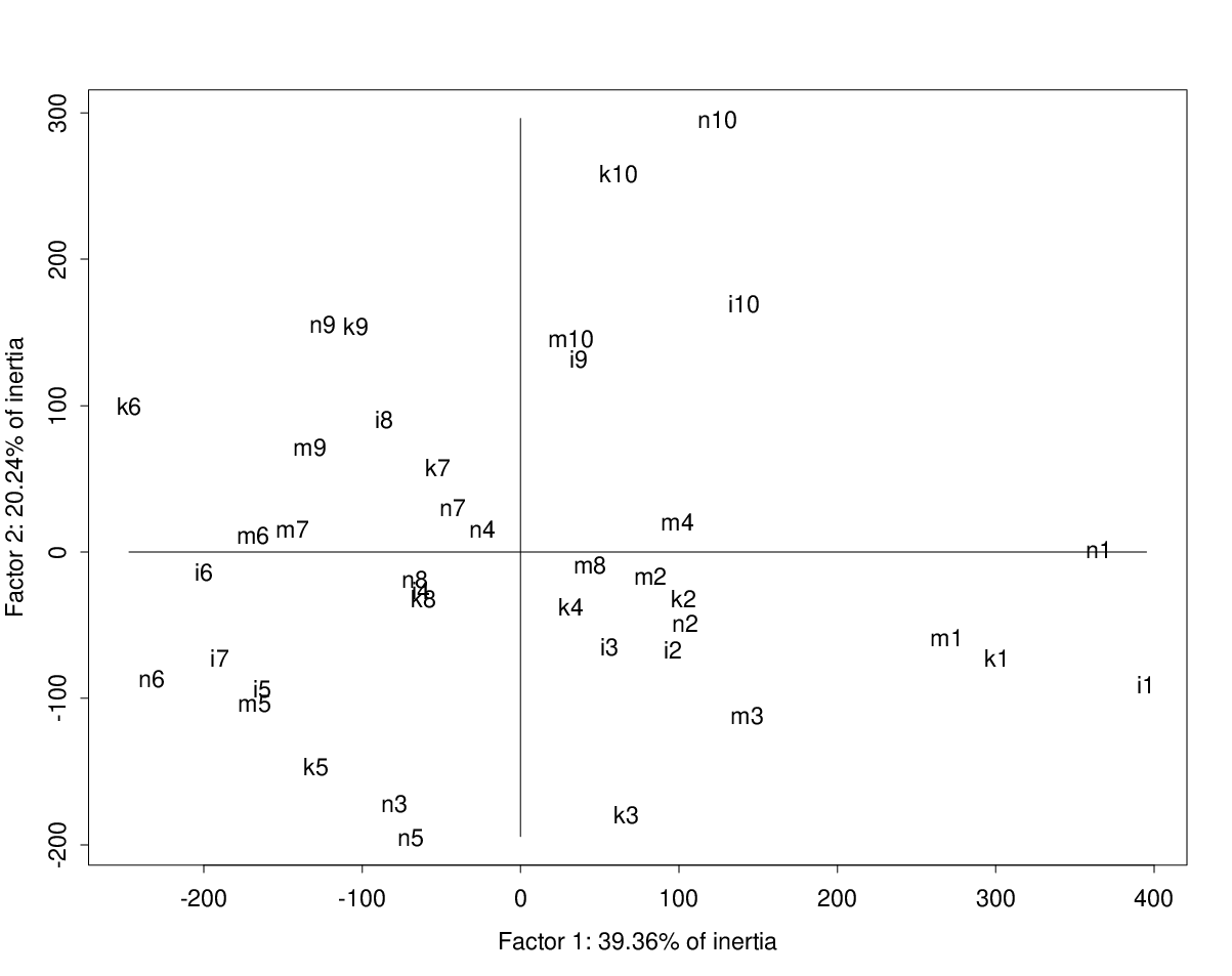
An analysis of clusters found is listed in Table 4. (Contributions to, and correlations with, the principal factors are used: see Murtagh, 2005, for a discussion of where these may differ from projections onto the factors. Projections, e.g. as shown in Figure 4, are descriptive: “what is?”, but correlations and contributions point to influence: “what causes?”. Correlations and contributions are used therefore, in preference to projections.)
In cluster 65, coding category 9 is predominant. In cluster 68, coding categories 2 and 3 are predominant. Cluster 69 is mixed. Cluster 70 is dominated by coding category 10. In cluster 71, coding category 8 is predominant. Cluster 72 is defined by coding category 1. Finally, cluster 73 is dominated by coding category 5.
            Clusters                       Quantile coding category

Cluster 65: k9 n9 k7 n7 i4 m9              Predominant: 9
Cluster 68: i3 k3 m3 m4 i2 m2 k2 n2        Predominant: 2, 3
Cluster 69: n6 i8 m7                       Predominant: none
Cluster 70: i10 m10 i9 k10 n10             Predominant: 10
Cluster 71: i6 k4 n4 m8 k8 n8              Predominant: 8
Cluster 72: i1 m1 k1 n1                    Predominant: 1
Cluster 73: i5 m5 n3 k5 n5 k6 i7 m6        Predominant: 5
From the clustering, we provisionally retain coding categories 1; 2 and 3 together; 5; 8; 9; and 10. We flag response categories 4, 6, and 7 as being unclear and best avoided when our aim is prediction of the futures data.
To check the coding relative to stationarity, we check that the global code boundaries are close to the time series sub-interval code boundaries. (See Murtagh, 2005, for more discussion on this, including confirmation of stationarity.) In broad terms, what we are checking here is the consistency of the representative elements, found in different subsets of the data, as illustrated above, right at the start of our presentation in this article, in Table 1.
12 Fingerprinting the Price Movements
Typical movements can be read off in percentage terms in a table such as Table 3. More atypical movements serve to define the strong patterns in our data.
We consider the clusters of current time-step code categories numbered 65, 68, 69, 70, 71, 72, 73 from Table 4, and we ask what are the likely movements, for one time step. Alternatively expressed the current code categories are defined at time step , and the one-step-ahead code categories are defined at time step .
We find the following predominant movements in Table 4 (using a thresholded contribution value – not shown here; we recall that “contribution” is used in the correspondence analysis sense, meaning mass times projection squared):
Cluster 65, i.e. code category 9: weakly 8 and more weakly 9.
Cluster 68, i.e. code categories 2 and 3: 7.
Cluster 69, i.e. mixed code categories: 6.
Cluster 70, i.e. code category 10: 10.
Cluster 71, i.e. code category 8: weakly 8.
Cluster 72, i.e. code category 1: 1.
Cluster 73, i.e. code category 5: 5
Consider the situation of using these results in an operational setting. From informative structure, we have found that code category 1 (values less than the 10th percentile, i.e. very low) has a tendency, departing from typical tendencies, to be prior to code category 1 (again very low). From any or all of tables such as Table 3 we can see how often we are likely to have this situation in practice: 19.04% (= average of 23.29% from Table 3, and 17.67%, 16.4%, and 18.8%, from the other analogous tables not shown here), given that we have code category 1.
Applying a similar fingerprinting analysis to Ross’s (2003) oil data, 749 values, we found that clustering the initial code categories did not make much sense: we retained therefore the trivial partition with all 10 code categories. For the output or one-step-ahead future code categories, we agglomerated 6 and 7, and denoted this cluster as 11. We find the following, generally weak, associations derived from the contributions.
Input code category 6 output code categories 1, 10 (weak).
Input code category 3 output code category 2.
Input code category 4 output code category 4.
Input code categories 9, 2 output code category 5 (weak).
Input code category 10 output code category 8.
Not surprisingly, we find very different patterns in the two data sets of different natures used, the futures and the oil price signals.
We have shown that structure can be discovered in data where such structure is not otherwise apparent. Furthermore we have used correspondence analysis, availing of its spatial projection and clustering aspects, as a convenient analysis environment. Validating the conclusions drawn is always most important, and this is facilitated by (i) semi-interactive data analysis, and (ii) consistency of results across subsets of the domain under investigation, .
13 Conclusions
Our new framework for data, and the handling of data (including our defining of a normed vector space), could be considered in a sense as “only” formalizing standard data analysis practice. But in the exploration and analysis of complex phenomena (cf. the search for local structure and patterns in price movements) we need to be sure of our belief in how our data express the underlying phenomena. The traditional Kolmogorov approach based on Lebesgue integration and sigma algebras of probability-measurable sets is unnecessarily abstract and therefore largely ignored by the “engineering” or pragmatic common sense of the data analyst.
In this article we have shown how the generalized Riemann integral lends itself to a more transparent definition of probability, in line with empirical data analysis practice. As a foundation for our data analysis tasks, it achieves a far better cohesiveness between data, and data analyses, vis à vis the underlying phenomena.
Acknowledgements
Some of this work was carried out in the project “Integration Methods in Financial Analysis”, supported by the British Council, UK, and the Polish State Committee for Scientific Research, KBN, Poland.
References
- 1.
J.P. Benzécri, L’Analyse des Données. Tome II. L’Analyse des Correspondances, 2nd ed., Dunod, 1976.
- 2.
J.P. Benzécri, Correspondence Analysis Handbook, Marcel Dekker, 1992.
- 3.
R. Gordon, The Lebesgue, Denjoy, Perron and Henstock Integrals, American Mathematical Society, 1994.
- 4.
R. Henstock, Lectures on the Theory of Integration, World Scientific, Singapore, 1988.
- 5.
R.N. Mantegna and H.E. Stanley, An Introduction to Econophysics, Cambridge University Press, 2000.
- 6.
P. Muldowney, A General Theory of Integration in Function Spaces, Pitman Research Notes in Mathematics no. 153, Harlow, 1988.
- 7.
P. Muldowney, Topics in probability using generalised Riemann integration, Mathematical Proceedings of the Royal Irish Academy, 99(B)1 (1999) 39–50.
- 8.
P. Muldowney, The Henstock integral and the Black-Scholes theory of derivative asset pricing, Real Analysis Exchange, 25(1) (2000/2001) 117–132
- 9.
P. Muldowney and V.A. Skvortsov, Lebesgue integrability implies generalized Riemann integrability in , Real Analysis Exchange, 27(1) (2001/2002) 223–234.
- 10.
F. Murtagh, Correspondence Analysis and Data Coding with R and Java, Chapman and Hall/CRC Press, 2005.
- 11.
S.M. Ross, An Elementary Introduction to Mathematical Finance, 2nd ed., Cambridge University Press, 2003.
- 12.
W. Rudin, Real and Complex Analysis, McGraw-Hill, New York, 1970.
- 13.
P.F. Velleman and L. Wilkinson, Nominal, ordinal, interval and ratio typologies are misleading, The American Statistician, 47 (1993) 65–72.