Partitioning Regular Polygons into Circular Pieces I:
Convex Partitions
Abstract
We explore an instance of the question of partitioning a polygon into pieces, each of which is as “circular” as possible, in the sense of having an aspect ratio close to . The aspect ratio of a polygon is the ratio of the diameters of the smallest circumscribing circle to the largest inscribed disk. The problem is rich even for partitioning regular polygons into convex pieces, the focus of this paper. We show that the optimal (most circular) partition for an equilateral triangle has an infinite number of pieces, with the lower bound approachable to any accuracy desired by a particular finite partition. For pentagons and all regular -gons, , the unpartitioned polygon is already optimal. The square presents an interesting intermediate case. Here the one-piece partition is not optimal, but nor is the trivial lower bound approachable. We narrow the optimal ratio to an aspect-ratio gap of with several somewhat intricate partitions.
1 Introduction
At the open-problem session of the 14th Canadian Conference on Computational Geometry,11 1 Lethbridge, Alberta, Canada, August 2002. the first author posed the question of finding a polynomial-time algorithm for partitioning a polygon into pieces, each with an aspect ratio no more than a given [DO03b]. The aspect ratio of a polygon is the ratio of the diameters of the smallest circumscribing circle to the largest inscribed indisk. (We will use “circumcircle” and “indisk” to emphasize that the former may overlap but the latter cannot.) If the pieces of the partition must have their vertices chosen among ’s vertices, i.e, if “Steiner points” are disallowed, then a polynomial-time algorithm is known [Dam02]. Here we explore the question without this restriction, but with two other restrictions: the pieces are all convex, and the polygon is a regular -gon. Although the latter may seem highly specialized, in fact many of the issues for partitioning an arbitrary polygon arise already with regular polygons. The specialization to convex pieces is both natural, and most in concert with the applications mentioned below. Partitions employing nonconvex pieces will be explored in [DO03a]. Our emphasis in this paper is not on algorithms, but on the partitions themselves.
1.1 Notation
A partition of a polygon is a collection of polygonal pieces such that and no pair of pieces share an interior point. To agree with the packing and covering literature, we will use for the aspect ratio, modified by subscripts and superscripts as appropriate. is the one-piece : the ratio of the radius of the smallest circumcircle of , to the radius of the largest disk inscribed in . is the maximum of all the for all pieces in a partition of ; so this is dependent upon the particular partition under discussion. Both the partition and the argument “” will often be dropped when clear from the context. is the minimum over all convex partitions of . Our goal is to find for the regular -gons.
To present our results, we introduce one more bit of notation, forward-referencing Section 2.2: is the “one-angle lower bound,” a lower bound derived from one angle of the polygon, ignoring all else. This presents a trivial lower bound on any partition’s aspect ratio.
1.2 Table of Results
Our results are summarized in Table 1. It makes sense that regular polygons for large are as circular as one could get. We prove that this holds true for all . For an equilateral triangle, the optimal partition can approach but never achieve the lower bound , for finite partitions. The square is an interesting intermediate case. Here the one-piece partition is not optimal, but nor is the trivial lower bound approachable. So . We narrow the optimal ratio to a small gap by raising the lower bound and lowering the upper bound.
| Regular Polygon | ||||
|---|---|---|---|---|
| Triangle | ||||
| Square | ? | |||
| Pentagon | ||||
| Hexagon | ||||
| Heptagon | ||||
| Octagon | ||||
| -gon | ||||
1.3 Motivation
Partitions of polygons into components that satisfy various shape criteria have been the focus of considerable research. Algorithms have been developed [Kei85] that produce partitions of simple polygons into the fewest convex polygons, spiral polygons, star-shaped polygons, or monotone polygons, when all the vertices of the partition pieces are selected from among the polygon vertices, i.e., Steiner points are not employed. Permitting Steiner points makes optimal partitions much more difficult to find. A notable success here is the polynomial-time algorithm of Chazelle and Dobkin [CD85], which partitions a simple polygon into the fewest number of convex pieces. See Keil [Kei00] and Bern [Ber97] for surveys of polygon partitioning.
Our motivation for investigating circular partitions is for their advantages in several application areas, for circular polygons have a number of desirable properties. Because they can be tightly circumscribed by a circle, they support quick collision detection tests, important in motion planning, dynamics simulations, and virtual reality. In graphics scenes containing a number of nonintersecting circular polygons, only a few might intersect a region small relative to the size of the polygons. This property has been used [SO94] to reduce the time complexity of a particular motion planning algorithm. Examples of other applications for which circular objects confer an advantage are range searching [OS96], simulation of physically-based motion [KHM+96], and ray tracing [FDFH96]. Partitions into circular pieces are relevant to all these applications.
Our focus on convex pieces is motivated by computational geometry applications that have simple and efficient and solutions if the input consists of convex pieces only. For instance, algorithms for collision detection, radiosity calculations, shading, and clipping run an order of magnitude faster on convex polygons than similar algorithms designed to handle arbitrary polygons. Convex polygons are also preferable in computer graphics because they are easy to represent, manipulate, and render.
There is an interesting connection between the problem studied in this paper and packings and coverings. For any partition of , the collection of indisks for each piece of the partition forms a packing of by disks, and the collection of circumcircles enclosing each piece form a covering of . We have found this connection to packing and covering more relevant when the pieces are not restricted to be convex [DO03a], but even for convex pieces it is at least suggestive. For example, the notorious difficulty of packing equal disks in a square may relate to the apparent difficulty of our problem for the square, which leads to a packing of the square with unequal disks. In any case, despite the connections, we have not found in the literature any work that directly addresses our particular problem.
1.4 Outline of Paper
Rather than follow the ordering in the table, we proceed in order of increasing difficulty: starting with the easiest result (pentagons and , Section 3), moving next to the equilateral triangle (Section 4), and finally to the square (Section 5). A preliminary section (Section 2) establishes some simple lemmas used throughout, and we look to the natural next steps for this work in a final Discussion, Section 6.
2 One-piece Partition and One-angle Lower Bound
First we establish two simple lemmas used throughout the rest of the paper.
2.1 One-piece Partition

Lemma 1
(Regular Polygon). The aspect ratio of a regular -gon is
Proof: Both the indisk and the circumcircle are centered on the polygon’s centroid. Referring to Figure 1, the angle formed by circumradius and inradius is . It follows immediately that .
2.2 One-angle Lower Bound

Lemma 2
(One-Angle Lower Bound). If a polygon contains a convex vertex of internal angle , then the aspect ratio of a convex partition of is no smaller than , with
Proof: Either the whole angle is included in one piece of the partition, or it is split and shared among several pieces. The latter gives an even lower bound. So consider the former.
Then the indisk must fit in the angle and the circumcircle must include the corner and surround the indisk; see Figure 2. We get a lower bound by maximizing the inradius and minimizing the circumradius. This happens when the indisk and the circumcircle are tangent where they intersect the bisector of the angle . Referring to Figure 2, the inradius is , the circumcircle’s diameter is and
From this we get , which concludes the lemma.
Note that cannot be achieved by a polygonal partition, a point to which we return in Lemma 4 below.
3 Pentagon
It is clear that for large enough , for a -gon. The only question is for which does this effect take over. The answer is :
Theorem 3
For a regular pentagon (), the optimal convex partition is just the pentagon itself, i.e., and .
Proof: The regular pentagon has (by the Regular Polygon Lemma 1). This is the -value for competitive partitions to beat.
- 1.
Suppose some piece has an edge incident to a vertex of the pentagon, and so splits the angle there. Then some piece has an angle . Lemma 2 then yields . Because this is larger than , no such partition could improve over .
- 2.
So assume there is a partition, none of whose edges are incident to a vertex of . We consider three cases for corner pieces: two acute, one acute, or both obtuse angles adjacent to .
- (a)
Suppose some piece of the partition that includes a vertex of contains two acute or right () angles adjacent to . Then this piece already exceeds , as is evident from Figure 3(a).


(a) (b) (c) Figure 3: Optimal pentagon partition (a) is insufficient to cover a corner piece with two right or acute angles adjacent to . (b) creates an angle in a piece adjacent to a corner piece with one acute and one obtuse angle (c) for a piece with two adjacent acute angles. Therefore every piece that encompasses a vertex of has at most one angle adjacent to .
- (b)
Suppose some piece of the partition that includes a vertex of contains one acute or right angle adjacent to . Note that here the one-angle lower bound Lemma 2 does not suffice to settle this case, as that yields . Suppose, to be generous, that this one nonobtuse angle is as large as possible, . Then if the exterior circle is to include the foot of that perpendicular and , then the adjacent piece must have an acute angle to the other side of , as simple geometric computations show; see Figure 3b. Applying Lemma 2 yields , which well exceeds . Thus that adjacent piece is inferior.
- (c)
Suppose every piece including a vertex of has only obtuse angles adjacent to . Then no two pieces containing adjacent vertices of can themselves be adjacent, for otherwise at their join along the side of , an angle would be obtuse on both sides. So there must be one or more intervening pieces. It is easy to see that, for each side of , one of these intervening pieces must have acute angles at both its corners on . For if the angle pairs alternate acute/obtuse, …, acute/obtuse, one of the corner pieces will have an acute angle on . Such a piece must have greater than the aspect ratio of a piece with right angles at both its corners on . From the right triangle in Figure 3c we get , which yields .
Having exhausted all cases, we are left with the conclusion that no partition can improve upon . Therefore .
- (a)
4 Equilateral Triangle
Recall from Table 1 that the one-angle lower bound for the equilateral triangle is . In this section we show that this lower bound can be approached, but never achieved, by a finite convex partition. That it cannot be achieved is a general result:
Lemma 4
For any polygon , the one-angle lower bound can never be achieved by a finite convex partition.
Proof: Recall from Figure 2 that is determined by a circumcircle tangent to an indisk nestled in the minimum angle corner of . Let be the point of tangency between these circles. As is clear from Figure 4, any partition piece covering and the corner must either lie exterior to or interior to in a neighborhood of . Either possibility forces .

Our proof that the lower bound of can be approached for an equilateral triangle follows five steps:
- 1.
suffices to partition any rectangle (Lemma 7).
- 2.
suffices to partition any “-quadrilateral” (Lemma 8).
- 3.
suffices to approximately partition the region between any pair of “-curves” (Lemma 10).
- 4.
The corners of an equilateral triangle can be covered by a polygon with as near to as desired (Figure 9a).
- 5.
The remaining “interstice” can be partitioned into regions bound by -curves (Figure 9b).
4.1 Rectangles
We first establish that permits partitioning of any rectangle. In fact, we prove that suffices.
Define the aspect ratio of a rectangle to be ratio of the length of its longer side to that of its shorter side. We start by noting that allows one-piece partitions for some aspect ratios strictly greater than .
Lemma 5
Any rectangle with has .
See Figure 5 where , and therefore .

Now we generalize to arbitrary aspect ratios, and return to below.
Lemma 6
Any rectangle may be partitioned into a finite number of rectangles, each with an aspect ratio of no more than , for any .
Proof: Let have dimensions , with . Define
| (1) | |||||
| (2) |
We want to cut up the long dimension into squares. Because , the portion left over can be absorbed by expanding each square by in that direction, for we know that . In other words, the left-over portion needs less than one more square to cover it, and the ’s suffice to give us this one more. We then arrange to slice the dimension into equal-sized strips whose width assures the desired . See Figure 6.

Lemma 7
Any rectangle may be partitioned into a finite number pieces with , for any .
Proof: Recall that for a square is . So any leaves a bit of slack, permitting rectangles of aspect ratio , for some , to have that . For example, Lemma 5 shows that for , . Now apply Lemma 6.
The number of pieces in the implied partition depends on , which depends on . For , each strip will have rectangles. Of course it is likely that much more efficient partitions are possible.
4.2 -Quadrilaterals
We next extend the rectangle lemma to slightly skewed quadrilaterals.
Lemma 8
There are quadrilaterals with one corner a right angle, and its opposite corner any angle within , which have .
Proof: Any quadrilateral fitting between the indisk and the circumcircle of Figure 5 satisfies . See Figure 7 for an example.

Define an -quadrilateral as one whose corner angles fall within .
Lemma 9
Any -quadrilateral may be partitioned with .
Proof: Partition into four “quarters” with orthogonal lines and through the centroid. We partition each quarter separately. Start at the exterior corner of , and create the largest quadrilateral satisfying Lemma 8, with the quadrilateral’s right angle flush against a quartering line, say . See piece in Figure 8. Continue in this manner, with each piece flush against , until the next piece would overlap into the next quarter ( and in the figure). Switch strategies to take a smaller piece flush with and the boundary of ( in the figure). Finally, we are left with a rectangle; cover according to Lemma 6.

4.3 -Curves
Define a pair of -curves and as two curves parametrized by , that satisfy the property that each segment whose endpoints are and , meets the curves at angles in the range .
Lemma 10
Let and be a pair of -curves. Then the region bounded by , , , and may be approximated to any given degree of accuracy by a region that can be finitely partitioned with .
Proof: Choose an and partition the range of into equal intervals. The quadrilaterals
for , satisfy Lemma 8 by hypothesis, and so each can individually be partitioned with . Clearly as , the approximation of to the region bounded by the curves improves in accuracy.
4.4 Partition of Interstice
The overall plan of the partition of an equilateral triangle is to first cover each -corner with a large convex polygon that approximates the lower bound. Figure 9a shows an example that is only above .
Three such pieces leave an “interstice” whose exact shape depends on how large the corner pieces are. In the center of the interstice (centered on the triangle centroid) we place a regular hexagon. Then the goal is to cover the remainder of the interstice, between the corner pieces and the hexagon, with . We will employ -curves near the hexagon; closer to the triangle side curves will not be necessary. The most difficult part of the construction is joining the curves to the hexagon. As Figure 9b illustrates, we partition the remaining exterior to each hexagon vertex into three angles. These provide termination points for the -curves.
 |
 |
|---|---|
| (a) | (b) |
The next task is to obtain an explicit form of the most critical pair of -curves, between the corner indisk and one of the curves incident to a hexagon corner. We choose to make this second curve an arc of a circle, although there are many choices. The construction starts with a circle and two radii from the horizontal. These radii bound a circular arc of angle , which meets the base of the hexagon in an angle, and extends down to line parallel to the base at another angle. See Figure 10a. The arc meets one of our criteria: it is incident to the hexagon at an angle. Now we consider paired with an arc of . Note that any segment incident to from the left, which starts within the shaded region , forms an angle with , because is delimited by rays from the endpoints of .

Now consider placing the center on the vertex of indicated in Figure 10b. We are going to partition the region between and with radial rays from the center of . Because the center of is in , all these rays satisfy the limit where they hit ; and of course they are orthogonal to . So the quadrilaterals determined by these rays are -quadrilaterals. Finally, as shown in Figure 10c, the angle of the uppermost quadrilateral incident to the hexagon corner is exactly , because was centered on a ray that achieves this. Therefore, we have in fact achieved the goal set out in Figure 9b: the exterior angle around the hexagon vertex is partitioned into three angles.
The overall design of the full partition is illustrated in Figure 11.

This figure shows several parts of the construction, but is not a full partition. The region is easily partitioned into -quadrilaterals by more radial rays from the center of . How many rays depends on the polygonal approximation to the corner piece; see again Figure 9a. The region can be partitioned by horizontal lines; again all the quadrilaterals are -quadrilaterals (see the lower angle in Figure 10a). The -curves terminate on the line through the centers of the two bottom incirles. Piece of the partition would again be partitioned by horizontal segments, as many as are needed to accomodate the polygonal approximation to there. Finally, the large remaining quadrilateral has base angles , and so is already an -quadrilateral. A possible partition into -quadrilaterals is shown in Figure 12.

We have established our theorem:
Theorem 11
An equilateral triangle may be partitioned into a finite number of pieces with ratio , for any . As approaches , the number of pieces goes to infinity.
5 Square
The square is intermediate between the equilateral triangle and the regular pentagon in several senses: (a) Unlike the pentagon, the one-piece partition is not optimal; (b) Unlike the equilateral triangle, the one-angle lower bound of (Table 1) cannot be approached. Although we believe a result similar to Theorem 11 holds—there is a lower bound that can be approached but not reached for a finite partition—we have only confined the optimal ratio to the range , leaving a gap of . We first show in Section 5.1 that the one-piece partition is not optimal through a series of increasingly complex partitions. Then we describe in Section 5.2 the example that establishes our upper bound . Section 5.3 presents the proof of the lower bound, . Finally, we close with a conjecture in Section 5.5 and supporting evidence.
5.1 Pentagons on Side
To improve upon the one-piece partition, pieces that have five or more sides must be employed, for the square itself is the most circular quadrilateral. One quickly discovers that covering the side of the square is challenging and crucial to the structure of the overall partition. We first explore partitions that use pentagons around the square boundary. Figure 13 shows a -piece partition, with a central octagon, that already improves upon , achieving ; but it is easily seen to be suboptimal.
 |
 |
|---|---|
| (a) | (b) |
Our next attempt, Figure 14, is a -piece partition improving to . It’s center is a near-regular -gon.
 |
 |
| (a) | (b) |
Our most elaborate pentagon example is the -piece partition shown in Figure 15, which achieves . It includes four heptagons adjacent to the corner pieces, and four dodecagons at the center, with all remaining pieces hexagons or pentagons. Note that throughout this series, the angle on the square side between the corner piece and its immediate neighbor is a critical angle. One wants this small so that the corner piece can be circular; but too small and the adjacent piece cannot be circular. It is exactly this tension that we will exploit in Section 5.3 to establish a lower bound.
 |
 |
We will leave it as a claim without proof that any square partition that covers the entire boundary of the square with pentagons must have . So Figure 15 cannot be much improved.
5.2 Hexagons on Side
To make further advances, it is necessary to move beyond pentagons. Figure 16 shows our best partition, which employs four corner pentagons and four hexagons along each side of the square. As is apparent from the figure, it is no longer straightforward to fill the interior after covering the boundary.

Figure 17 shows the indisks and circumcircles for the pieces of the partition. Only the central tear-drop shape and the corner pieces on the “second level” have significant slack with respect to the achieved .

We again leave it as claim without proof that further improvements here will not be large: any square partition that covers the entire boundary of the square with hexagons must have .
5.3 Lower Bound on
One quickly develops a sense that the lower bound provided by Lemma 2, , is not approachable. We derive here a larger lower bound, , by focussing on the piece adjacent to a corner piece, which we call a “bottleneck piece.”
Theorem 12
The optimal aspect ratio for a convex partition of a square is at least
The proof is in three steps. Let , , and be the first three piece vertices along the bottom square side, with the square corner, as in Figure 18.
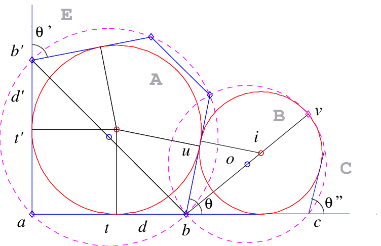
We first derive a lower bound by concentrating on only (Lemma 13), and then improve that by focussing on as well (Lemma 14). Finally, we show that this bound applies to any partition (Lemma 15).
Lemma 13
Pieces and of Figure 18 (the corner piece and the bottleneck piece) must satisfy
Proof: Let the inscribed circle for the partition piece that covers the corner have radius . We know that . We will show that in fact .
Let be the piece adjacent to along the bottom side of the square. The angles of the two pieces at their shared square side point are supplementary: the internal angle at in is . The lower bound derives from the angle of , but if , then the lower bound for the piece is larger. So we compute two bounds on as functions of : one for piece and one for piece . The overall optimum is achieved when these two bounds are in balance. So we set them equal and solve for . We then use to compute .
Let and be the partition pieces adjacent to and along the bottom and left side of the square respectively (see again Figure 18). Without loss of generality, we make two assumptions:
- (a)
the internal angle of at point is no greater than the internal angle of at point ; otherwise, we can balance the aspect ratios of and to get a larger .
- (b)
the internal angle of at point is no less that the internal angle of at point ; otherwise, we can balance the aspect ratios of and to get a larger .
First we derive as a function of . We must have and therefore the distance between points and in Figure 18 is:
| (3) |
Similarly, the distance between and is , or
| (4) |
A’s circumradius is , which together with (3) and (4) yields
| (5) |
For the piece , the lower bound Lemma 2 yields:
| (6) |
To minimize , we balance the bounds and and solve for theta. From this we get and .
 (a)
(b)
(a)
(b)
Lemma 14
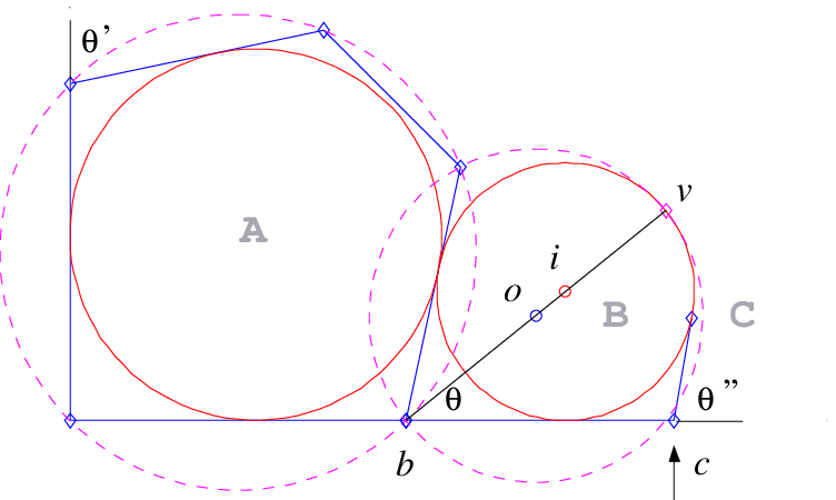
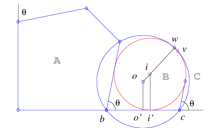
Pieces and of Figure 19 (the corner piece and the bottleneck piece) must satisfy
Proof: Simple calculations show that for the value from Lemma 13, ’s circumcircle does not include point of interior angle in , as illustrated in Figure 19a. So in fact is too large; ’s circumcircle is too small: two points (, ) do not suffice to define ’s circumcircle.
Based on this observation, we force ’s circumcircle to pass through three points: , and the tangency point with the indisk (which may not lie on the bisector of ). Refer to Figure 19b. This leads to a new value , which we compute next. To minimize , we force . Throughout the rest of the proof we let the origin be determined by point and set .
Let and be ’s circumcenter and incenter, respectively. Then . The distance between points and in Figure 19b is . The distance between points and is . The projection of on falls in the middle of . The three points , and all lie on a straight line, since is a common tangency point for the indisk and the circumcircle. Thus the distance between the incenter and the circumcenter is . Putting all these together leads to the following system of equations:
Solving this for yields . From we compute and , where is a complex expression on . We balance this with from (5) and solve for . This yields22 2 Mathematica finds an exact expression for the solution, but we only report its numerical value here. . From we compute , which completes the proof.
Lemma 15
Any convex partition of a a square satisfies , i.e., the lower bound from Lemma 15 cannot be achieved.
Proof: The lower bound derives from square side piece with interior angles adjacent to the square side equal to and . Now consider the sequence of pieces along the bottom square side. At some point the pieces in this sequence have to straighten up as they approach the right corner of the square. This idea is illustrated in Figure 20, in which angles adjacent to the horizontal square side have values, from left to right
Such straightening implies that there is a piece with interior angles adjacent to the bottom square side equal to and , with . Such a piece has ratio strictly greater than .

This completes the proof of Theorem 12.
Figure 21a shows a coverage of the full square boundary that achieves , only above the optimal . This gap is determined by the bottleneck piece shown in Figure 21b. To narrow the gap further, and must approach the optimal angle value established in Theorem 12, and more points must be added in the vicinity of the tangency point between the indisk and the circumcircle. This shows that the lower bound can be approached as the number of pieces goes to infinity, but only covering the square boundary. As the number of pieces along the square sides increases, it becomes less clear how to fill the interior with the same ratio.
 |
 |
| (a) | (b) |
5.4 Tangent Indisks
In this section we present some evidence that the lower bound established in Theorem 12 might not be attained. We specialize the discussion to the situation where all the indisks touching the square side are tangent to their left and right neighbors. Although this is a very natural constraint, notice in Figure 18 that balancing the -ratios for pieces and leads to indisks that are not mutually tangent. Of course each is tangent to the edge shared between and , but those tangency points do not coincide exactly. The advantage of considering tangent indisks is that this added bit of structural constraint allows some analytical calculations, rather than relying on numerical optimizations. Because these investigations are inconclusive, we include no proofs. The end result, in Conjecture 1 below, is a larger lower bound for tangent indisks.
First, we compute the for an indisk sandwiched between parallel tangents:
Lemma 16
Let an indisk of radius sit on a horizontal line , supported on the left and right by tangents that both meet in angle . Then the smallest circumcircle that includes the indisk, and the foot of both tangents, has radius , with
The minimum value is achieved when , when .

Next we derive a relationship between the angle of the separating tangent line and the disk radii; see Figure 22.
Lemma 17
Let two disks, of radius and , touch a horizontal line , and touch each other. Then the line of tangency between them is slanted toward the smaller disk, making an angle with the horizontal, and meeting midway between the projection of the centers of the two disks, with

Third, we compute the angle at the next “level” between two adjacent pieces, as a function of the tangent slant and ; see Figure 23.
Lemma 18
Let two tangent indisks, of radius and , sit on a horizontal line , supported by three slanted tangents that all meet in angle . Let the origin be determined by the leftmost tangent’s intersection with . Let be the middle tangent, with . Let circumcircles of radius and surround the indisks and pass through the feet of the tangents on . Let be the point on that is highest above and inside both circumcircles and the angle determined by and the upper tangents to the two disks. Then , as a function of and , is
where

Finally, the above three lemmas permit us to start with a of and compute backwards. This leads to a lower bound in the “tangent indisks” model where we tune so that the next-level angle is . See Figure 24.
Conjecture 1
The optimal aspect ratio for a partition of a square into convex pieces with tangent indisks along the sides of the square is .
The idea here is that with this , we have duplicated the corner of the square at the next level, leaving the remaining problem of covering the interior as difficult as the original.
5.5 Square: Discussion
Results of Sections 5.1–5.3 show that finding an optimal aspect ratio partition of a square is not straightforward. It remains open to narrow the gap between the lower bound of provided by Lemma 12 and the upper bound of established by Figure 16.
 |
 |
| (a) | (b) |
As mentioned, it seems feasible to lower the upper bound of the gap to a value slightly larger than , the optimal value for any partition that covers the entire square boundary with hexagons. For instance, Figure 25 shows a coverage of the full square boundary that achieves , which is only above the optimal for hexagons. We conjecture that a construction similar to that in Figure 16 can be used to fill in the interior.
To narrow the gap further, it is necessary to employ pieces with more than six vertices along the boundary of the square. However, Figure 21 suggests that pieces with a large number of vertices along square sides create a large discrepancy in segment lengths bounding the interior. Filling the interior then becomes problematic. However we see no fundamental impediment to doing so. Based on partial results not reported in this paper, we would be surprised if the optimal partition could be achieved with a finite partition:
Conjecture 2
No finite partition achieves the optimal partition of the square: rather can be approached as closely as desired as the number of pieces goes to infinity.
6 Discussion
This paper establishes the optimally circular convex partition of all regular polygons, except for the square, where we have left a small gap. We hope to show in future work that our results apply to arbitrary polygons as well. We have also investigated nonconvex circular partitions of regular polygons [DO03a].
Our work leaves many problems unresolved:
- 1.
Narrow the gap for the optimal aspect ratio of a convex partition of a square.
- 2.
Determine for the square if , the number of pieces in an optimal partition, is finite or infinite (cf. Conjecture 1).
- 3.
For each , find the optimal ratio of a polygon using only convex -gons. It is especially interesting to determine for a -gon. For example, Figure 13 and work not reported here shows that for a square. We did not explore for an equilateral triangle; it would be interesting to replace the corner pieces in Figure 12 with quadrilaterals.
- 4.
For each , find the optimal ratio of a polygon using convex pieces. So each of our partitions of the square establishes a particular upper bound, e.g., Figure 14 shows that .
- 5.
More generally, develop a tradeoff between the number of pieces of the partition and the circularity ratio achieved.
- 6.
Extend our results to all convex polygons, and then to arbitrary polygons.
Finally, all these problems could be fruitfully explored in 3D, the natural dimension for the applications discussed in Section 1.3.
References
- [Ber97] M. Bern. Triangulations. In J.E. Goodman, , and J. O’Rourke, editors, Handbook of Discr. Comp. Geom., chapter 22, pages 413–428. CRC Press LLC, Boca Raton, FL, 1997.
- [CD85] B. Chazelle and D. P. Dobkin. Optimal convex decompositions. In G. T. Toussaint, editor, Computational Geometry, pages 63–133. North-Holland, Amsterdam, Netherlands, 1985.
- [Dam02] M. Damian. Exact and approximation algorithms for computing optimal -fat decompositions. In Proc. 14th Canad. Conf. Comput. Geom., pages 93–96, August 2002.
- [DO03a] M. Damian and J. O’Rourke. Partitioning regular polygons into circular pieces II: Nonconvex partitions, 2003. In preparation.
- [DO03b] E.D. Demaine and J. O’Rourke. Open problems from CCCG 2002. In Proc. 15th Canad. Conf. Comput. Geom., 2003. To appear. arXiv cs.CG/0212050. http://arXiv.org/abs/cs/0212050/.
- [FDFH96] J.D. Foley, A.v. Dam, S.K. Feiner, and J.F. Huges. Computer Graphics: Principles and Practice (2nd edition in C). Addison Wesley, 1996.
- [Kei85] J.M. Keil. Decomposing a polygon into simpler components. SIAM J. on Comp., 14:799–817, 1985.
- [Kei00] J.M. Keil. Polygon decomposition. In J.-R. Sack and J. Urrutia, editors, Handbook of Computational Geometry, chapter 11, pages 491–518. Elsevier, 2000.
- [KHM+96] J.T. Klosowski, M. Held, J.S.B. Mitchell, H. Sowizral, and K. Zikan. Real-time collision detection for motion simulation within complex environments. ACM Siggraph Vis. Proc., 14:151, 1996.
- [OS96] M.H. Overmars and A.F. Stappen. Range searching and point location among fat objects. J. of Algh., 21(3):629–656, 1996.
- [SO94] A.F. Stappen and M.H. Overmars. Motion planning amidst fat obstacles. Proc. of the 10th ACM Symp. Comput. Geom., pages 31–40, 1994.