Fault-tolerant Routing in Peer-to-peer SystemsThis is an extended version of the paper appearing in the proceedings of the Twenty-First ACM Symposium on Principles of Distributed Computing, 2002
Abstract
We consider the problem of designing an overlay network and routing mechanism that permits finding resources efficiently in a peer-to-peer system. We argue that many existing approaches to this problem can be modeled as the construction of a random graph embedded in a metric space whose points represent resource identifiers, where the probability of a connection between two nodes depends only on the distance between them in the metric space. We study the performance of a peer-to-peer system where nodes are embedded at grid points in a simple metric space: a one-dimensional real line. We prove upper and lower bounds on the message complexity of locating particular resources in such a system, under a variety of assumptions about failures of either nodes or the connections between them. Our lower bounds in particular show that the use of inverse power-law distributions in routing, as suggested by Kleinberg [5], is close to optimal. We also give efficient heuristics to dynamically maintain such a system as new nodes arrive and old nodes depart. Finally, we give experimental results that suggest promising directions for future work.
1 Introduction
Peer-to-peer systems are distributed systems without any central authority and with varying computational power at each machine. We study the problem of locating resources in such a large network of heterogeneous machines that are subject to crash failures. We describe how to construct distributed data structures that have certain desirable properties and allow efficient resource location.
Decentralization is a critical feature of such a system as any central server not only provides a vulnerable point of failure but also wastes the power of the clients. Equally important is scalability: the cost borne by each node must not depend too much on the network size and should ideally be proportional, within polylogarithmic factors, to the amount of data the node seeks or provides. Since we expect nodes to arrive and depart at a high rate, the system should be resilient to both link and node failures. Furthermore, disruptions to parts of the data structure should self-heal to provide self-stabilization.
Our approach provides a hash table-like functionality, based on keys that uniquely identify the system resources. To accomplish this, we map resources to points in a metric space either directly from their keys or from the keys’ hash values. This mapping dictates an assignment of nodes to metric-space points. We construct and maintain a random graph linking these points and use greedy routing to traverse its edges to find data items. The principle we rely on is that failures leave behind yet another (smaller) random graph, ensuring that the system is robust even in the face of considerable damage. Another compelling advantage of random graphs is that they eliminate the need for global coordination. Thus, we get a fully-distributed, egalitarian, scalable system with no bottlenecks.
We measure performance in terms of the number of messages sent by the system for a search or an insert operation. The self-repair mechanism may generate additional traffic, but we expect to amortize these costs over the search and insert operations. Given the growing storage capacity of machines, we are less concerned with minimizing the storage at each node; but in any case the space requirements are small. The information stored at a node consists only of a network address for each neighbor.
The rest of the paper is organized as follows. Section 2 explains our abstract model in detail, and Section 3 describes some existing peer-to-peer systems. We prove our results for routing in Section 4. In Section 5, we present a heuristic method for constructing the random graph and provide experimental results that show its performance in practice. Section 6 describes results of experiments we performed to test the routing performance of our constructed distributed data structure. Conclusions and future work are discussed in Section 7.
2 Our approach
The idea underlying our approach consists of three basic parts: (1) embed resources as points in a metric space, (2) construct a random graph by appropriately linking these points, and (3) efficiently locate resources by routing greedily along the edges of the graph. Let be a set of resources spread over a large, heterogeneous network . For each resource , denotes the node in that provides and denotes the resource’s key. Let be the set of all possible keys. We assume a hash function such that resource maps to the point in a metric space , where is the point set and is the distance metric as shown in Figure 1. The hash function is assumed to populate the metric space evenly. Note that via this resource embedding, a node is mapped onto the set , namely the set of metric-space points assigned to the resources the node provides.

Our next step is to carefully construct a directed random graph from the points embedded in . We assume that each newly-arrived node is initially connected to some other node in . Each node generates the outgoing links for each vertex independently. A link simply denotes that knows that is the network node that provides the resource mapped to ; hence, we can view the graph as a virtual overlay network of information, pieces of which are stored locally at each node. Node constructs each link by executing the search algorithm to locate the resource that is mapped to the sink of that link. If the metric space is not populated densely enough, the choice of a sink may result in a vertex corresponding to an absent resource. In that case, chooses the neighbor present closest to the original sink. Moving to nearby vertices will introduce some bias in the link distribution, but the magnitude of error does not appear to be large. A more detailed description of the graph construction is given in Section 5.
Having constructed the overlay network of information, we can now use it for resource location. As new nodes arrive, old nodes depart, and existing ones alter the set of resources they provide or even crash, the resources available in the distributed database change. At any time , let be the set of available resources and be the corresponding overlay network. A request by node to locate resource at time is served in a simple, localized manner: calculates the metric-space point that corresponds to , and a request message is then routed over from the vertex in that is closest to to itself.11 1 Note that since generally changes with time, and may specifically change while the request is being served, the request message may be routed over a series of different overlay networks . Each node needs only local information, namely its set of neighbors in , to participate in the resource location. Routing is done greedily by forwarding the message to the node mapped to a metric-space point as close to as possible. The problem of resource location is thus translated into routing on random graphs embedded in a metric space.
To a first approximation, our approach is similar to the “small-world” routing work by Kleinberg [5], in which points in a two-dimensional grid are connected by links drawn from a normalized power-law distribution (with exponent 2), and routing is done by having each node route a packet to its neighbor closest to the packet’s destination. Kleinberg’s approach is somewhat brittle because it assumes a constant number of links leaving each node. Getting good performance using his technique depends both on having a complete two-dimensional grid of nodes and on very carefully adjusting the exponent of the random link distribution. We are not as interested in keeping the degree down and accept a larger degree to get more robustness. We also cannot assume a complete grid: since fault-tolerance is one of our main objectives, and since nodes are mapped to points in the metric space based on what resources they provide, there may be missing nodes.
The use of random graphs is partly motivated by a desire to keep the data structure scalable and the routing algorithm as decentralized as possible, as random graphs can be constructed locally without global coordination. Another important reason is that random graphs are by nature robust against node failures: a node-induced subgraph of a random graph is generally still a random graph; therefore, the disappearance of a vertex, along with all its incident links (due to failure of one of the machines implementing the data structure) will still allow routing while the repair mechanism is trying to heal the damage. The repair mechanism also benefits from the use of random graphs, since most random structures require less work to maintain their much weaker invariants compared to more organized data structures.
Embedding the graph in a metric space has the very important property that the only information needed to locate a resource is the location of its corresponding metric-space point. That location is permanent, both in the sense of being unaffected by disruption of the data structure, and easily computable by any node that seeks the resource. So, while the pattern of links between nodes may be damaged or destroyed by failure of nodes or of the underlying communication network, the metric space forms an invulnerable foundation over which to build the ephemeral parts of the data structure.
3 Current peer-to-peer systems
Most of the peer-to-peer systems in widespread use are not scalable. Napster [8] has a central server that services requests for shared resources even though the actual resource transfer takes place between the peer requesting the resource and the peer providing it, without involving the central authority. However, this has several disadvantages including a vulnerable single point of failure, wasted computational power of the clients as well as not being scalable. Gnutella [1] floods the network to locate a resource. Flooding creates a trade-off between overloading every node in the network for each request and cutting off searches before completion. While the use of super-peers [7] ameliorates the problem somewhat in practice, it does not improve performance in the limit.
Some of these first-generation systems have inspired the development of more sophisticated ones like CAN [11], Chord [13] and Tapestry [2]. CAN partitions a -dimensional metric space into zones. Each key is mapped to a point in some zone and stored at the node that owns the zone. Each node stores information, and resource location, done by greedy routing, takes time. Chord maps nodes to identities of bits placed around a modulo identifier circle. Resources are stored at existing successor nodes of the nodes they are mapped to. Each node stores a routing table with entries such that the -th entry stores the key of the first node succeeding it by at least on the identifier circle. Each resource is also mapped onto the identifier circle and stored at the first node succeeding the location that it maps to. Routing is done greedily to the farthest possible node in the routing table, and it is not hard to see that this gives an delivery time with nodes in the system. Tapestry uses Plaxton’s algorithm [10], a form of suffix-based, hypercube routing, as the routing mechanism: in this algorithm, the message is forwarded deterministically to a node whose identifier is one digit closer to the target identifier. To this end, each node maintains pieces of information and delivery time is also .
Although these systems seem vastly different, there is a recurrent underlying theme in the use of some variant of an overlay metric space in which the nodes are embedded. The location of a resource in this metric space is determined by its key. Each node maintains some information about its neighbors in the metric space, and routing is then simply done by forwarding packets to neighbors closer to the target node with respect to the metric. In CAN, the metric space is explicitly defined as the coordinate space which is covered by the zones and the distance metric used is simply the Euclidean distance. In Chord, the nodes can be thought of being embedded on grid points on a real circle, with distances measured along the circumference of the circle providing the required distance metric. In Tapestry, we can think of the nodes being embedded on a real line and the identifiers are simply the locations of the nodes on the real line. Euclidean distance is used as the metric distance for greedy forwarding to nodes with identifiers closest to the target node. This inherent common structure leads to similar results for the performance of such networks. In this paper, we explain why most of these systems achieve similar performance guarantees by describing a general setting for such overlay metric spaces, although most of our results apply only in one-dimensional spaces.
In general, the fault-tolerance properties of these systems are not well-defined. Each system provides a repair mechanism for failures but makes no performance guarantees till this mechanism kicks in. For large systems, where nodes appear and leave frequently, resilience to repeated and concurrent failures is a desirable and important property. Our experiments show that with our overlay space and linking strategies, the system performs reasonably well even with a large number of failures.
4 Routing
In this section, we present our lower and upper bounds on routing. We consider greedy routing in a graph embedded in a line where each node is connected to its immediate neighbors and to multiple long-distance neighbors chosen according to a fixed link distribution. We give lower bounds for greedy routing for any link distribution satisfying certain properties (Theorem 10). We also present upper bounds in the same model where the long-distance links are chosen as per the inverse power-law distribution with exponent and analyze the effects on performance in the presence of failures.
4.1 Tools
Some of our upper bounds will be proved using a well-known upper bound of Karp et al.[3] on probabilistic recurrence relations. We will restate this bound as Lemma 1, and then show how a similar technique can be used to get lower bounds with some additional conditions in Theorem 2.
Lemma 1 ([3])
The time needed for a nonincreasing real-valued Markov chain to drop to is bounded by
| (1) |
when is a nondecreasing function of .
This bound has a nice physical interpretation. If it takes one second to jump down meters from , then we are traveling at a rate of meters per second during that interval. When we zip past some position , we are traveling at the average speed determined by our starting point for the interval. Since is nondecreasing, using as our estimated speed underestimates our actual speed when passing . The integral computes the time to get all the way to zero if we use as our instantaneous speed when passing position . Since our estimate of our speed is low (on average), our estimate of our time will be high, giving an upper bound on the actual expected time.
We would like to get lower bounds on such processes in addition to upper bounds, and we will not necessarily be able to guarantee that , as defined in Lemma 1, will be a nondecreasing function of . But we will still use the same basic intuition: The average speed at which we pass is at most the maximum average speed of any jump that takes us past . We can find this maximum speed by taking the maximum over all ; unfortunately, this may give us too large an estimate. Instead, we choose a threshold for “short” jumps, compute the maximum speed of short jumps of at most for all between and , and handle the (hopefully rare) long jumps of more than by conditioning against them. Subject to this conditioning, we can define an upper bound on the average speed passing , and use essentially the same integral as in (1) to get a lower bound on the time. Some additional tinkering to account for the effect of the conditioning then gives us our real lower bound, which appears in Theorem 2 below, as Inequality (8).
Theorem 2
Let be Markov process with state space , where is a constant. Let be a non-negative real-valued function on such that, for all ,
| (2) |
Let and be constants such that for any ,
| (3) |
Let
| (4) |
For each with , let satisfy
| (5) |
Now define
| (6) |
and define
| (7) |
Then
| (8) |
Proof: Define
| (9) |
The idea is that drops to zero immediately if a long jump occurs. We will show that even with such overeager jumping, does not drop too quickly on average. The intuition is that the chance of a long jump reduces by at most an expected , while the effect of short jumps can be bounded by applying the definition of .
Let be the -algebra generated by . Let be the event that , that is, that the jump from to is a short jump. Now compute
| (10) | |||||
Now, conditioning on means that and thus for the entire range of the integral. It follows that lies in the half-open interval for each such , from which we have from (6). Inverting gives , and plugging this inequality into (11) gives
| (12) | |||||
We have now shown that drops slowly on average. To turn this into a lower bound on the time at which it first reaches zero, define . Conditioning on , observe that
Alternatively, if we have
In either case, , implying . In other words, is a submartingale.
Because is a submartingale, and is a stopping time relative to , we have . Solving for then gives
4.2 Lower bounds on greedy routing
We will now show a lower bound on the expected time taken by greedy routing on a random graph embedded in a line. Each node in the graph has expected outdegree at most and is connected to its immediate neighbor on either side. For polylogarithmic values of , we consider two variants of the greedy routing algorithm and derive lower bounds for them equal to and to , as stated in Theorem 10. The routing variants, along with the machinery and proofs of the associated lower bounds, are presented in Sections 4.2.1 through 4.2.6. For large values of , a lower bound of on the worst-case routing time can be derived very simply, as follows.
Theorem 3
Let . Then for any link distribution and any routing strategy, the delivery time .
Proof: With links for each node, we can reach at most nodes at step . Assuming that the minimum time to reach all nodes is T, . This gives a lower bound of on .
4.2.1 Lower bound for polylogarithmic number of links
We consider the case of the expected outdegree of each node falling in the range . The probability that a node at position is connected to positions depends only on the set and not on and is independent of the choice of outgoing links for other nodes.22 2 We assume that nodes are labeled by integers and identify each node with its label to avoid excessive notation. Since we assume that each node is connected to its immediate neighbors, we require that appears in .
We consider two variants of the greedy routing algorithm. Without loss of generality, we assume that the target of the search is labeled . In one-sided greedy routing, the algorithm never traverses a link that would take it past its target. So if the algorithm is currently at and is trying to reach , it will move to the node with the smallest non-negative label. In two-sided greedy routing, the algorithm chooses a link that minimizes the distance to the target, without regard to which side of the target the other end of the link is. In the two-sided case the algorithm will move to a node whose label has the smallest absolute value, with ties broken arbitrarily. One-sided greedy routing can be thought of as modeling algorithms on a graph with a boundary when the target lies on the boundary, or algorithms where all links point in only one direction (as in Chord).
Our results are stronger for the one-sided case than for the two-sided case. With one-sided greedy routing, we show a lower bound of on the time to reach from a point chosen uniformly from the range to that applies to any link distribution. For two-sided routing, we show a lower bound of , with some constraints on the distribution. We conjecture that these constraints are unnecessary, and that is the correct lower bound for both models. A formal statement of these results appears as Theorem 10 in Section 4.2.6, but before we can prove it we must develop machinery that will be useful in the proofs of both the one-sided and two-sided lower bounds.
4.2.2 Link sets: notation and distributions
First we describe some notation for sets. Write each as
where whenever . Each is a random variable drawn from some distribution on finite sets; the individual are thus in general not independent. Let consist of the negative elements of and consist of the positive elements. Formally define when and when .
For one-sided routing, we make no assumptions about the distribution of except that must have finite expectation and always contains . For two-sided routing, we assume that is generated by including each possible in with probability , where is symmetric about the origin (i.e., for all ), , and is unimodal, i.e. nonincreasing for positive and nondecreasing for negative .33 3 These constraints imply that ; formally, we imagine that is present in each but is ignored by the routing algorithm. We also require that the events and are pairwise independent for distinct .
4.2.3 The aggregate chain
For a fixed distribution on , the trajectory of a single initial point is a Markov chain , with , where determines the outgoing links from the node reached at time and is a successor function that selects the next node according to the routing algorithm. Note that the chain is Markov, because the presence of links guarantees that no node ever appears twice in the sequence, and so each new node corresponds to a new choice of links.
From the chain we can derive an aggregate chain that describes the collective behavior of all nodes in some range. Each state of the aggregate chain is a contiguous sets of nodes whose labels all have the same sign; we define the sign of the state to be the common sign of all of its elements. For one-sided routing each state is either or an interval of the form for some . For two-sided routing the states are more general The aggregate states are characterized formally in Lemma 5.
Given a contiguous set of nodes and a set , define
The intuition is that consists of all those nodes for which the algorithm will choose as the outgoing link. Note that will always be a contiguous range because of the greediness of the algorithm. Now define, for each :
Here we have simply split into those nodes with negative, zero, or positive successors.
For any set and integer write for .
We will now build our aggregate chain by letting the successors of a range be the ranges for all possible , , and . As a special case, we define when ; once we arrive at the target, we do not leave it. For all other , we let
| (14) |
and define the unconditional transition probabilities by averaging over all .
Lemma 4 shows that moving to the aggregate chain does not misrepresent the underlying single-point chain:
Lemma 4
Let be drawn uniformly from the range . Let be a uniformly chosen element of . Then for all and , .
Proof: Clearly the lemma holds for . Fix , and consider two methods for generating . The first generates directly from and shows that generated in this way has the same distribution as . The second generates from as describe in the lemma and produces the same distribution on as the first.
In the first method, we choose uniformly from , choose a random , and compute . Here the transition rule applied to is the same as for , so under the induction hypothesis that and are equal in distribution, so are and .
In the second method, we again choose a random and then choose by choosing some in proportion to its size, let , and then let be a uniformly chosen element of . We can implement the choice of by choosing some uniformly from and picking as the subrange that contains ; and we can simplify the task of choosing by setting it equal to , since conditioning on leaves with a uniform distribution. But by implementing the second method in this way, we have reduced it to the first, and the lemma is proved.
Lemma 5 justifies our earlier characterization of the aggregate state spaces:
Lemma 5
Let for some . Then with one-sided routing, every is either or of the form for some ; and with two-sided routing, every is an interval of integers in which every element has the same sign.
Proof: By induction on . For one-sided routing, observe that is always empty, as the routing algorithm is not allowed to jump to negative nodes. If , then . Otherwise ; but since for some , if it contains any point greater than it must contain ; thus and so becomes .
The result for the two-sided case is immediate from the fact that combined with the definition of .
The advantage of the aggregate chain over the single-point chain is that, while we cannot do much to bound the progress of a single point with an arbitrary distribution on , we can show that the size of does not drop too quickly given a bound on . The intuition is that each successor set of size or less occurs with probability at most , and there are at most such sets on average.
Lemma 6
Let . Then for any , in either the one-sided or two-sided model,
| (15) |
Proof:
Fix . First note that if , then . So we can assume that and in particular that .
Conditioning on , there are at most non-empty sets . If , then is chosen with probability at most by (14). Thus the probability of choosing any of the at most sets of size at most is at most .
Now observe that
4.2.4 Boundary points
Lemma 6 says that seldom drops by too large a ratio at once, but it doesn’t tell us much about how quickly drops in short hops. To bound this latter quantity, we need to get a bound on how many subranges splinters into through the action of . We will do so by showing that only certain points can appear as the boundaries of these subranges in the direction of .
For fixed , define for each
and
Let be the set of all finite and .
Lemma 7
Fix and and let be defined as above. Suppose that is positive. Let be the set of minimum elements of subranges of . Then is a subset of and contains no elements other than
- 1.
,
- 2.
for each ,
- 3.
for each , and
- 4.
at most one of or for each ,
where the last case holds only with two-sided routing.
If is negative, the symmetric condition holds for .
Proof: Consider some subrange of . If contains , the first case holds. Otherwise: (a) if , the second case holds; (b) if , the third case holds; (c) if , the fourth case holds, with if is odd, and either or if is even, depending on whether the tie-breaking rule assigns to or .
We will call the elements of boundary points of .
4.2.5 Bounding changes in
Now we would like to use Lemmas 6 and Lemma 7 to get an upper bound on the rate at which drops as a function of the distribution.
The following lemma is used to bound a sum that arises in Lemma 9.
Lemma 8
Let . Let where each and at least one is greater than Let be the set of all for which is greater than . Then
| (16) |
Proof: If , we still have for all , so the left-hand side cannot be less than . So the interesting case is when .
Let have elements. Then and . Because is convex, its sum over is minimized for fixed by setting all such equal, in which case the left-hand side of (16) becomes simply for any .
Now observe that setting all in equal gives .
Lemma 9
Fix , and let be a positive range with . Define as in Lemma 7. Let . Let be the event . Then
| (17) |
where with one-sided routing and with two-sided routing.
Proof: Call a subrange large if and small otherwise; the intent is that the large ranges are precisely those that yield . Observe that for any large , , implying any large set has at least two elements.
For any large , . Similarly . So any large intersects in at least one point.
Let be the set of subranges , large or small, that intersect . It is immediate from this definition that and thus .
Using Lemma 7, we can characterize the elements of as follows.
- 1.
There is at most one set that contains .
- 2.
There is at most one set that has for each in .
- 3.
There is at most one set that has for each in .
- 4.
With two-sided routing, there is at most one set that has or for each in . Note that there may be a set whose minimum element is where , but this set is already accounted for by the first case.
Thus has at most elements with one-sided routing and at most elements with two-sided routing.
Conditioning on , is equal to for some large and thus for some large . Which large is chosen is proportional to its size, so for fixed , we have
where the first inequality follows from Lemma 8.
Now let us compute
In the second-to-last step, we use , which follows from . In the last step, we use , which follows from the concavity of and Jensen’s inequality.
4.2.6 Putting the pieces together
We now have all the tools we need to prove our lower bound.
Theorem 10
Let be a random graph whose nodes are labeled by the integers. Let for each be a set of integer offsets chosen independently from some common distribution, subject to the constraint that and are present in every , and let node have an outgoing link to for each . Let . Consider a greedy routing trajectory in starting at a point chosen uniformly from and ending at .
With one-sided routing, the expected time to reach is
| (18) |
With two-sided routing, the expected time to reach is
| (19) |
provided is generated by including each in with probability , where (a) is unimodal, (b) is symmetric about , and (c) the choices to include particular are pairwise independent.
Proof: Let .
We are going to apply Theorem 2 to the sequence with . We have chosen so that when we reach the target, ; so that a lower bound on gives a lower bound on the expected time of the routing algorithm. To apply the theorem, we need to show that (a) the probability that drops by a large amount is small, and (b) that the integral in (7) is large.
For the second step, Theorem 2 requires that we bound the speed of the change in solely as a function of . For one-sided routing this is not a problem, as Lemma 5 shows that , which reveals , characterizes exactly except when and the lower bound argument is done. For two-sided routing, the situation is more complicated; there may be some which is not of the form or , and we need a bound on the speed at which drops that applies equally to all sets of the same size.
It is for this purpose (and only for this purpose) that we use our conditions on for two-sided routing. Suppose that each appears in with probability , that these probabilities are pairwise-independent, and that the sequence is symmetric and unimodal. Let , where , the absolute ceiling of , is when and when . Observe that ; in effect, we are counting in all midpoints of pairs of distinct elements of without regard to whether the elements are adjacent. For each , the expected number of distinct pairs , with and is at most ; this is a convolution of the non-negative, symmetric, and unimodal sequence with itself and so it is also symmetric and unimodal. It follows that for all , , and similarly .
Now for the punch line: for each , is an upper bound on the expected number of distinct pairs that put in , which is in turn an upper bound on , and from the unimodularity of we have that and whenever . Though grossly over counts the elements of (in particular, it gives a bound on of ), its ordering property means that we can bound the expected number of elements of that appear in some subrange of any positive by using to bound the expected number of elements that appear in the corresponding subrange of , and similarly for negative and . Because already satisfies a similar ordering property, we can thus bound the number of elements of both and that hit a fixed subrange of given only . We do this next.
For convenience, formally define and for one-sided routing. We will simplify some of the summations by first summing the and over certain pre-defined intervals. For each integer let . Let . Note that for one-sided routing and for two-sided routing. Observe also that is at most for one-sided routing and at most for two-sided routing.
Consider some . Let be the event . If , then by Lemma 9 we have
| (20) |
where with one-sided routing and with two-sided routing, with in each case, as in Lemma 9.
As we observed earlier, our choice of and Lemma 6 imply , so for sufficiently large . So we can replace (20) with
| (21) |
Let us now obtain a bound on in terms of and the and . For one-sided routing, we use the fact that implies . For two-sided routing, we use monotonicity of the and to replace with ; in particular, to replace a sum of over a subrange of with a sum over subrange of that is at least as large. In either case, we get that
| (22) |
and thus is bounded by
| (23) |
provided . For , set .
Let us now compute , as defined in (6). For , . For larger , observe that . Now if , then the bounds on the sum in (23) both lie between and , so that
where .
Finally, compute
To get a lower bound on the sum, note that
which is at most for one-sided routing and at most for two-sided routing. In either case, because is convex and decreasing, we have
| (24) | |||||
We will now rewrite our bound on in a more convenient asymptotic form. We will ignore the and concentrate on the large fraction. Recall that , so . Unless is polynomial in , we have and the numerator simplifies to .
Now let us look at the denominator. Consider first the term . We can rewrite this term as ; since goes to zero as and grow we have . It is unlikely that this term will contribute much.
Turning to the second term, let us use the fact that for . Thus
and the bound in (24) simplifies to . We can further assume that , since otherwise the bound degenerates to , and rewrite it simply as
4.2.7 Possible strengthening of the lower bound
Examining the proof of Theorem 10, both the that appears in the bound (19) for two-sided routing and the extra conditions imposed on the distribution arise only as artifacts of our need to project each range onto and thus reduce the problem to tracking a single parameter. We believe that a more sophisticated argument that does not collapse ranges together would show a stronger result:
Conjecture 11
Let , , and be as in Theorem 10. Consider a greedy routing trajectory starting at a point chosen uniformly from and ending at .
Then the expected time to reach is
with either one-sided or two-sided routing, and no constraints on the distribution.
We also believe that the bound continues to hold in higher dimensions than . Unfortunately, the fact that we can embed the line in, say, a two-dimensional grid is not enough to justify this belief; divergence to one side or the other of the line may change the distribution of boundaries between segments and break the proof of Theorem 10.
4.3 Upper Bounds
In this section, we present upper bounds on the delivery time of messages in a simple metric space: a one-dimensional real line. To simplify theoretical analysis, the system is set up as follows.
- •
Nodes are embedded at grid points on the real line.
- •
Each node is connected to its nearest neighbor on either side and to one or more long-distance neighbors.
- •
The long-distance neighbors are chosen as per the inverse power-law distribution with exponent , i.e., each long-distance neighbor is chosen with probability inversely proportional to the distance between and . Formally, Pr[ is the th neighbor of ] = , where is the distance between nodes and in the metric space.
- •
Routing is done greedily by forwarding the message to the neighbor closest to the target node.
We analyze the performance for the cases of a single long-distance link and of multiple ones, both in a failure-free network and in a network with link and node failures. Note that when we say node, we actually refer to a vertex in the virtual overlay network and not a physical node as in the earlier sections.
4.3.1 Single Long-Distance Link
We first analyze the delivery time in an idealized model with no failures and with one long-distance link per node. Kleinberg [5] proved that with nodes embedded at grid points in a -dimensional grid, with each node connected to its immediate neighbors and one long-distance neighbor chosen with probability proportional to , any message can be delivered in time polynomial in using greedy routing. While this result can be directly applied to our model with and to give a delivery time, we get a much simpler proof by use of Lemma 1. We include the proof below for completeness.
Theorem 12
Let each node be connected to its immediate neighbors (at distance 1) and long-distance neighbor chosen with probability inversely proportional to its distance from the node. Then the expected delivery time with nodes in the network is .
Proof: Let be the expected number of nodes crossed when the message is at a node that is at a distance from the destination. Clearly, is non-decreasing.

Let
where
Then
Clearly, is non-decreasing, and thus using Lemma 1, we get
Thus with this distribution, the delivery time is logarithmic in the number of nodes.
4.3.2 Multiple Long-Distance Links
The next interesting question is whether we can improve the delivery time by using multiple links instead of a single one. In addition to improvement in performance, multiple links also give the benefit of robustness in the face of failures. We first look at improvement in performance by using multiple links in the system and then go onto analysis of failures in Section 4.3.3. Suppose that there are links from each node. We consider different strategies for generating links and routing depending on number of links in two ranges: and .
In [6], Kleinberg uses a group structure to get a delivery time of for the case of a polylogarithmic number of links. However, he uses a more complicated algorithm for routing while we obtain the same bound (for the case of a line) using only greedy routing.
4.3.2.1 Upper Bound
Let us first consider a randomized strategy for link distribution when .
Theorem 13
Let each node be connected to its immediate neighbors (at distance 1) and long-distance neighbors chosen independently with replacement with probability proportional to their distances from the node. Let . Then the expected delivery time .
Proof: The basic idea for this proof comes from Kleinberg’s model [5]. Kleinberg considers a two-dimensional grid with nodes at every grid point. The delivery of the message is divided into phases. A message is said to be in phase if the distance from the current node to the destination node is between and . There are at most () such phases. He proves that the expected time spent in each phase is at most , thus giving a total upper bound of on the delivery time. We use the same phase structure in our model, and this proof is along similar lines.
In our multiple-link model, each node has long-distance neighbors chosen with replacement. The probability that chooses a node as its long-distance neighbor is , where . We can get a lower bound on this probability as follows:
Notice that , because and . So, the probability that chooses as its long-distance neighbor is at least
Now suppose that the message is currently in phase . To end phase at this step, the message should enter a set of nodes at a distance of the destination node . There are at least nodes in , each within distance of . So the message enters with probability
Let be the total number of steps spent in phase . Then
Now if denotes the total number of steps, then , and by linearity of expectation, we get .
For , we use a deterministic strategy. We represent the location of each node as a number in a base , and generate links to nodes at distances , for each . Routing is done by eliminating the most significant digit of the distance at each step. As this distance can be at most , we get . This strategy is similar in spirit to Plaxton’s algorithm [10].
Some special cases are instructive. Let and let each node link to nodes in both directions at distances , provided nodes are present at those distances. This gives . Similarly let . Links are established in both directions to existing nodes at distances , giving . In fact, when , for any fixed .
Theorem 14
Choose an integer . With , let each node link to nodes at distances , for each . Then the delivery time .
Proof: Let be the distances of the successive nodes in the delivery path from the target , where is the distance of the source node and . For each such that
Hence
Now each node is connected to the node at distance . We get
Thus drops by at least 1 at every step. As , we get .
4.3.3 Failure of Links
It appears that our
linking strategies may fail to give the same delivery time
in case the links fail. However, we show that we get reasonable
performance even with link failures. In our model, we assume
that each link is present independently with probability .
Let us first look at
the randomized strategy for number of links .

Our proof is along similar lines as our proof for the case of no failures. Intuitively, since some of the links fail, we expect to spend more time in each phase and this time should be inversely proportional to the probability with which the links are present. We prove that the expected time spent in one phase is , which gives a total delivery time of . We assume that the links to the immediate neighbors are always present so that a message is always delivered even if it takes very long.
Theorem 15
Let the model be as in Theorem 13. Assume that the links to the immediate neighbors are always present. If the probability of a long-distance link being present is , then the expected delivery time is .
Proof: Recall that in case of no link failures, the probability that chooses a node as its long-distance neighbor is at least where .
Now when we consider link failures, given that chose as its long-distance neighbor, the probability that there is a link present between and is . So, the probability that chooses a node as its long-distance neighbor is at least .
The rest of the proof is the same as the proof for theorem 13. Let be the number of steps spent in phase . Then
If denotes the total number of steps, then by linearity of expectation, we get .
We turn to the deterministic strategy with links. A similar intuition works for . If a link fails, then the node has to take a shorter long-distance link, which will not take the message as close to the target as the initial failed link. Clearly as decreases, the message has to take shorter and shorter links which increases the delivery time.
To make the analysis simpler, we change the link model a bit and let each node be connected to other nodes at distances . Once again, we compute the expected distance covered from the current node and use Lemma 1 to get a delivery time of . As decreases, the delivery time increases; whereas as decreases, the delivery time decreases, but the information stored at each node increases.
Theorem 16
Let the number of links be , and let each node have a link to distances . Assume that the links to the nearest neighbors are always present. If the probability of a link being present is , then the delivery time .
Proof: Let the distance of the current node from the destination be . Let represent the distance covered starting from this node. Then with probability , there will be a link covering distance . If this link is absent with probability , then we can cover a distance with a single link with probability and so on. In general, the average distance covered when the message is at distance from the destination is
Using Lemma 1, we get
4.3.4 Failure of Nodes
We consider two different cases of node failures when we study their effect on system performance. In the first case, as described in Section 4.3.4.1, some of the nodes may fail and then the remaining nodes will link to each other as per the link distribution. In the second case, as explained in Section 4.3.4.2, the nodes first link to their neighbors and then some of the nodes may fail.
4.3.4.1 Binomially Distributed Nodes
Let be the probability that a node is present at any point. Here also, each node is connected to its nearest neighbors and one long-distance neighbor. In addition, the probability of choosing a particular node as a long-distance neighbor is conditioned on the existence of that node.
Theorem 17
Let the model be as in Theorem 12. Let each node be present with probability and all nodes link only to existing nodes. Then the worst-case expected delivery time is .
Proof: We bound the expected drop as follows:
Using Lemma 1, we get . This is exactly the same result that we get in Section 4.3.1 where all the nodes are present.
This result is not surprising because if nodes link only to other existing nodes, the only difference is that we get a smaller random graph. This does not affect the routing algorithm or the delivery time.
4.3.4.2 General Failures
We observe that the analysis for node failures is not as simple as that for link failures because we no longer have the important property of independence that we have in the latter case. In the case of link failures, the nodes first choose their neighbors and then it is possible that some of these links fail; thus, the event that a node is connected to another node is completely independent of the event that, say, its neighbor is connected to the same node. Each link fails independently, and so the accessibility of a target node from any other node depends only on the presence of the link between the two nodes in question.
In case of node failures, this important independence property is no longer true. Suppose that a node cannot communicate with some other node (because failed), even though there may be a functional link between and . Now the probability of some other node being able to communicate with is not independent of the probability that can communicate with because the probability of being absent is common for both the cases. This complicates the analysis of the performance because it is no longer the case that if one node cannot communicate with some other node, it has a good chance of doing so by passing the message to its neighbor.
In order to analyze this situation, we consider jumps only to one phase lower rather than jumping over several phases. The idea is that the jumps between phases are independent, so once we move from phase to phase , further routing no longer depends on any nodes in phase . We can condition on the number of nodes being alive in the lower phase and estimate the time spent in each phase. Intuitively, if a node is present with probability , we would expect to wait for a time inversely proportional to in anticipation of finding a node in the lower phase to jump to.
Theorem 18
Let the model be as in Theorem 13 and let each node fail with probability . Then the expected delivery time is .
Proof: Let be the time taken to drop down from layer to layer . Let out of nodes be alive in layer and let be the probability that a node in layer is connected to some node in layer . Then the expected time to drop to layer , given that there are live nodes in it, is given by
Now can vary between and . (Note that cannot be because if there are no live nodes in the lower layer, the routing fails at this point.) We get
Not surprisingly, the expected waiting time in a layer is inversely proportional to the probability of being connected to a node in the lower layer and to the probability of such a node being alive.
For our randomized routing strategy with links, . Since there are at most layers, we get an expected delivery time of .
In contrast, for our deterministic routing strategy, certain carefully chosen node failures can lead to dismal situations where a message can get stuck in a local neighborhood with no hope of getting out of it or eventually reaching the destination node. We conjecture that this should be a very low probability event, so its occurrence will not affect the delivery time considerably. We have not yet analyzed this situation formally.
5 Construction of Graphs
As the group of nodes present in the network changes, so does the graph of the virtual overlay network. In order for our routing techniques to be effective, the graph must always exhibit the property that the likelihood of any two vertices being connected is . We describe a heuristic approach to construct and maintain a random graph with such an invariant.
Since the choice of links leaving each vertex is independent of the choices of other vertices, we can assume that points in the metric space are added one at a time. Let be the -th point to be added. Point chooses the sinks of its outgoing links according to the inverse power law distribution with exponent and connects to them by running the search algorithm. If a desired sink is not present, connects to ’s closest live neighbor. In effect, each of the points already present before is surrounded by a basin of attraction, collecting probability mass in proportion to its length. Since we assume the hash function populates the metric space evenly, and because of absolute symmetry, the basin length has the same distribution for all points. It is easy to see that with high probability, will not be much smaller than its expectation: . A lower bound on the probability that the link is present is , where is the point in ’s basin that is the farthest from .44 4 The constant has absorbed and the normalizing constant for the distribution. However, the bound holds only if is among the points added before . Otherwise, the aforementioned probability is , which means that we need to amend our linking strategy to transfer probability mass from the case of having arrived before to the case of having arrived after . We describe next how to accomplish this task.
Let be a new point. We give earlier points the opportunity to obtain outgoing links to by having (1) calculate the number of incoming links it ‘‘should’’ have from points added before it arrived, and (2) choose such points according to the inverse power-law distribution with exponent 1.55 5 All this can be easily calculated by since the link probabilities are symmetric. If is the number of outgoing links for each point, then will also be the expected number of incoming links that has to estimate in step (1). We approximate the number of links ending at by using a Poisson distribution with rate , that is, the probability that has incoming links is , and the expectation of the distribution is .
After step (2) is completed by , each chosen point responds to ’s request by choosing one of its existing links to be replaced by a link to . The choice of the link to replace can vary. We use a strategy that builds on the work of Sarshar et al.[12]. In that work, the authors use ideas of Zhang et al.[15] to build a graph where each node has a single long-distance link to a node at distance with probability . When a node with a long-distance link at distance encounters a new node at distance , either due to its arrival or due to a data request, it replaces its existing link with probability , where , and links to the new node. We extend this idea to our case of multiple long-distance links. Consider a node with neighbors at distances . When a new node at distance requests an incoming link from , replaces one of its existing links with a link to with probability . This is a trivial extension of the formula of [12]. However, this probability must now be distributed among ’s existing long-distance links since needs to choose one of them to redirect to . We choose to do that according to the inverse power-law distribution with exponent 1, that is, chooses to replace its link to the node at distance , , with probability . Hence, the probability that decides to link to and decides to replace its existing link to the node at distance with a link to is equal to . Notice that may decide not to redirect any of its existing links to with probability . The intuition for using such replacement strategy comes from the invariant that we want to maintain dynamically as new nodes arrive: has a link to a node at distance with probability inversely proportional to ; hence, conditioning on having long-distance links, the following equation must hold.
The same heuristic can be used for regeneration of links when a node crashes.
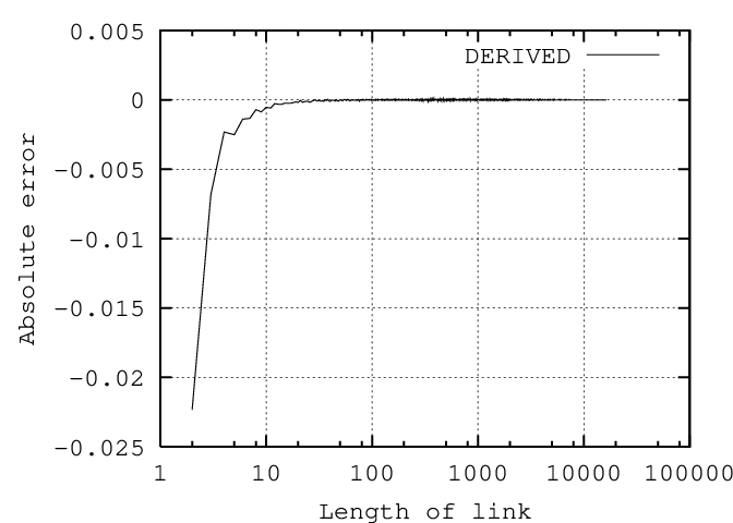
To analyze the performance of the heuristic in practice, we used it to construct a network of nodes with links each, ten separate times. After averaging the results over the ten networks, we plotted the distribution of long-distance links derived from the heuristic, along with the ideal inverse power-law distribution with exponent 1, as shown in Figure 5(a). We see that the derived distribution tracks the ideal one very closely, with the largest absolute error being roughly equal to for links of length , as shown in the graph of Figure 5(b).
We also performed experiments for an alternative link replacement strategy: a node chooses its oldest link to replace with a link to the new node. The performance of this strategy is almost as good as the performance of our replacement strategy described previously. We omit those results because it is difficult to distinguish between the results of the two strategies on the scale used for our graphs.
There has also been other related work [9] on how to construct, with the support of a central server, random graphs with many desirable properties, such as small diameter and guaranteed connectivity with high probability. Although it is not clear what kind of fault-tolerance properties this approach offers if the central server crashes, or how the constructed graph can be used for efficient routing, it is likely that similar techniques could be useful in our setting.

6 Experimental Results
We simulated a network of nodes at the application level. Each node is connected to its immediate neighbors and has long-distance links chosen as per the inverse power law distribution with exponent as explained in Section 4.3. Routing is done greedily by forwarding a message to the neighbor closest to its target node. In each simulation, the network is set up afresh, and a fraction of the nodes fail. We then repeatedly choose random source and destination nodes that have not failed and route a message between them. For each value of , we ran simulations, delivering messages in each simulation, and averaged the number of hops for successful searches and the number of failed searches.
With node failures, a node may not be able to find a live neighbor that is closer to the target node than itself. We studied three possible strategies to overcome this problem as follows.
- 1.
Terminate the search.
- 2.
Randomly choose another node, deliver the message to this new node and then try to deliver the message from this node to the original destination node (similar to the hypercube routing strategy explained in [14]).
- 3.
Keep track of a fixed number (in our simulations, ) of nodes through which the message is last routed and backtrack. When the search reaches a node from where it cannot proceed, it backtracks to the most recently visited node from this list and chooses the next best neighbor to route the message to.
For all these strategies we note that once a node chooses its best neighbor, it does not send the message to any other link if it finds out that the best neighbor has failed.


Figure 6 shows the fraction of messages that fail to be delivered and the number of hops for successful searches versus the fraction of failed nodes. We see that the system behaves well even with a large number of failed nodes. In addition, backtracking gives a significant improvement in reducing the number of failures as compared to the other two methods, although it may take a longer time for delivery. We see that in the case of random rerouting, the average delivery time does not increase too much as the probability of node failure increases. This happens because quite a few of the searches fail, so the ones that succeed (with a few hops) lead to a small average delivery time.
Our results may not be directly comparable to those of CAN[11] and Chord[13], since they use different simulators for their experiments. However, to the extent that the results are comparable, our methods appear to perform as well as theirs. Even if we just terminate the search, we get less than fraction of failed searches with fraction of failed nodes. Chord[13] has roughly the same performance after their network stabilizes using their repair mechanism. Further, with backtracking we see that with failed nodes, we still get less than failed searches. These results are very promising and it would be interesting to study backtracking analytically.
We also compared the performance of the ideal network and that of the network constructed using the heuristics given in Section 5. We ran iterations of constructing a network of nodes, both ideally as well as according to the heuristic, and delivered messages between randomly chosen nodes. Figure 7 shows the number of failed searches as the probability of node failure increases. We see that although the network constructed using the heuristic does not perform as well as the ideal network, the number of failed searches is comparable.

7 Conclusions and Future Work
| Model | Number of Links | Upper Bound | Lower Bound |
| No failures | 1 | ||
| Pr[Link present]= | - | ||
| - | |||
| Pr[Node present]= | - |
Table 7 summarizes our upper and lower bounds. We have shown that greedy routing in an overlay network organized as a random graph in a metric space can be a nearly optimal mechanism for searching in a peer-to-peer system, even in the presence of many faults. We see this as an important first step in the design of efficient algorithms for such networks, but many issues still need to be addressed. Our results mostly apply to one-dimensional metric spaces like the line or a circle. One interesting possibility is whether similar strategies would work for higher-dimensional spaces, particularly ones in which some of the dimensions represent the actual physical distribution of the nodes in real space; good network-building and search mechanisms for this model might allow efficient location of nearby instances of a resource without having to resort to local flooding (as in [4]). Another promising direction would be to study the security properties of greedy routing schemes to see how they can be adapted to provide desirable properties like anonymity or robustness against Byzantine failures.
8 Acknowledgments
The authors are grateful to Ben Reichardt for pointing out an error in an earlier version of Lemma 9.
References
- [1] GNUTELLA. http://gnutella.wego.com.
- [2] A. D. Joseph, J. Kubiatowicz, and B. Y. Zhao. Tapestry: An infrastructure for fault-tolerant wide-area location and routing. Technical Report UCB/CSD-01-1141, University of California, Berkeley, Apr 2001.
- [3] R. M. Karp, E. Upfal, and A. Wigderson. The complexity of parallel search. Journal of Computer and System Sciences, 36(2):225–253, 1988.
- [4] D. Kempe, J. M. Kleinberg, and A. J. Demers. Spatial gossip and resource location protocols. In Proceedings of 33rd Annual ACM Symposium on Theory of Computing, pages 163–172, Crete, Greece, July 2001.
- [5] J. Kleinberg. The small-world phenomenon:an algorithmic perspective. In Proceedings of 32nd Annual ACM Symposium on Theory of Computing, pages 163–170, Portland, Oregon, USA, May 2000.
- [6] J. Kleinberg. Small-world phenomena and the dynamics of information. In T. G. Dietterich, S. Becker, and Z. Ghahramani, editors, Advances in Neural Information Processing Systems 14, Cambridge, MA, 2002. MIT Press.
- [7] MORPHEUS. http://www.musiccity.com.
- [8] NAPSTER. http://www.napster.com.
- [9] G. Panduragan, P. Raghavan, and E. Upfal. Building low-diameter P2P networks. In Proceedings of 42nd Annual IEEE Symposium on the Foundations of Computer Science (FOCS), pages 492–499, Las Vegas, Nevada, USA, Oct. 2001.
- [10] C. Plaxton, R. Rajaram, and A. W. Richa. Accessing nearby copies of replicated objects in a distributed environment. In Proceedings of the Ninth Annual ACM Symposium on Parallel Algorithms and Architectures (SPAA), pages 311–320, Newport, RI, USA, June 1997.
- [11] S. Ratnasamy, P. Francis, M. Handley, R. Karp, and S. Shenker. A scalable content-addressable network. In Proceedings of the ACM SIGCOMM, pages 161–170, San Diego, CA, USA, Aug. 2001.
- [12] N. Sarshar and V. Roychowdhury. A random structure for optimum cache size distributed hash table (DHT) peer-to-peer design. Oct. 2002. http://arxiv.org/abs/cs.NI/0210010.
- [13] I. Stoica, R. Morris, D. Karger, F. Kaashoek, and H. Balakrishna. Chord: A scalable peer-to-peer lookup service for internet applications. In Proceedings of SIGCOMM 2001, pages 149–160, San Diego, CA, USA, Aug. 2001.
- [14] L. Valiant. A scheme for fast parallel communication. SIAM Journal on Computing, 11:350–361, 1982.
- [15] H. Zhang, A. Goel, and R. Govindan. Using the small-world model to improve freenet performance. In Proceedings of the IEEE INFOCOM, New York, NY, USA, June 2002.