On the survey-propagation equations for the random K-satisfiability problem
Abstract
In this note we study the existence of a solution to the survey-propagation equations for the random K-satisfiability problem for a given instance. We conjecture that when the number of variables goes to infinity, the solution of these equations for a given instance can be approximated by the solution of the corresponding equations on an infinite tree. We conjecture (and we bring numerical evidence) that the survey-propagation equations on the infinite tree have an unique solution in the suitable range of parameters.
1 Introduction
Recently many progresses [1, 2] have been done on the analytic and numerical study of the random K-satisfiability problem [3, 4, 5, 6], using the approach of survey-propagation that generalizes the more old approach based on the ‘‘Min-Sum’’ 11 1 The “Min-Sum” is the the zero temperature limit of the “Sum-Product” algorithm and sometimes is also called belief propagation. In the statistical mechanics language [8] the belief propagation equations are the extension of the TAP equations for spin glasses [14] and the survey-propagation equations are the TAP equations generalized to the broken replica case. algorithm [7, 8, 9, 10] .
The aim of this note is to sketch a possible path to a proof of the existence an uniqueness of the survey-propagation equations for a given instance of the problem. Before presenting the main arguments, for reader convenience I will present an heuristic derivation of the survey-propagation equations in section 2; the full derivation can be found in the original papers [1, 2, 11, 12, 13]. In section 3, I will present the main sequence of conjectures that may lead to the proof of the existence and uniqueness of the survey-propagation equations in the appropriate range of parameters. Finally I will present some conclusions.
2 A fast heuristic derivation of the survey equations
2.1 The random K-sat problem
In the random K-sat problem there are variable that may be true of false (the index will sometime called a node). An instance of the problem is given by a set of clauses. Each clause is characterized by set of three nodes (,, ), that belong to the interval and by three Boolean variables (,, ). In the random case the and variables are random with flat probability distribution. Each clause is true if the expression
| (1) |
is true. The problem is satisfiable iff we can find a set of the variables such that all the clauses are true. The entropy [10] of a satisfiable problem is the logarithm of the number of the different sets of the variables that make all the clauses true.
To a given problem we can associate a graph (the factor graph [9]) where the nodes are connected to the clauses ( in average) and each clause is connected to three nodes. The properties of this graph play a very important role.
The goal of the analytic approach consists in finding for given and for large values of the probability that a random problem (i.e. a problem with random chosen clauses) is satisfiable. The law [4, 6, 15] is supposed to be valid: for all systems (with probability one when goes to infinity) are satisfiable and their entropy is proportional to with a constant of proportionality that does not depend on the problem. On the other hand, for no random system (with probability one) is satisfiable. An heuristic argument has been given [1, 2] that suggest that where can be computed using the survey-propagation equations defined later. There is already an incomplete proof [16] that is a rigorous upper bound to .
2.2 The belief propagation equations
In the following analysis it will be crucial that in limit the problem becomes locally trivial: this makes possible the computations of and of the other properties of the system. Let us be more precise. We can define a distance among the nodes in the following way:
- •
Two nodes are at distance 1 if there is a clause that contains both of them. At large the number of nodes at distance 1 from a given node has a Poisson distribution with average .
- •
Two nodes are at distance if they are not at a distance and there is a chain of overlapping clauses that touch both of them (or equivalently the second node is at distance 1 from a node at distance from the first node).
In the limit the set of nodes at distance from a given node form a tree, without closed loops: locally the system looks like a tree. The solution of the K-sat problem on a tree (with given boundary conditions) can be trivially done: the belief propagation algorithm (defined later) is exact. When goes to infinity the systems is not a tree (with probability 1) and this fact makes hard to find an actual solution of the problem for a given instance; it may even destroy the global existence of a solution to the belief propagation equations. However the local treeness of the problem is enough to allow an analytic treatment.
Let us take a large system for and let us consider the set of all configurations that satisfies all the clauses. Our first task is to compute the probabilities and that the variable is true or false (obviously ), if belong to a random configuration in .
The presence of a simple local structure allows us to write down simple local equations [11, 12, 13]. In the case of belief propagation equation [7] one proceed as follows. For each clause that contains the node (we will use the notation although it may be not the most appropriate) is the probability that the variable would be true in absence of the clause . If the node were contained in only one clause, we would have that
| (2) |
where is an appropriate function that is defined by the previous relation. An easy computation shows that when all the are false, the variable must be true if both variable and are false, otherwise it can have any value. Therefore we have in this case that
| (3) |
In a similar way, if some of the variable are true, we should exchange the with the for the corresponding variables. Finally we have that
| (4) |
In total there are variables and equations. These equations are called in the literature under different name (e.g. belief propagation, TAP equations [14]) and we naively expect that these equations (belief propagations) are satisfied (or quasi-satisfied, i. e. corrections of order can be present [13]). For the time being let us suppose that such a solution exists and it is unique. In such case we expect that
| (5) |
We note the previous formulae can be written in a more compact way if we introduce a two dimensional vector , with components and . We define the product of these vector
| (6) |
if .
If the norm of a vector is defined by
| (7) |
we finally find that
| (8) |
For each clause we can define the probability that the clause would be satisfied in a system where the clause is not present. We will denote this probability by . One finds that in the case where all the variables are false
| (9) |
Finally the total entropy (apart correction that are subleading when goes to infinity) is given by
| (10) |
2.3 The survey propagation equations
One can argue that the situation is more complex [8, 12, 13]. The belief propagation algorithm works at low value of but it fails when becomes too large. The previous equations may have multiple solutions or quasi-solutions that are very different one from the other.
This fact has been interpreted [1, 2, 12, 13] in the following way: the set of all configurations that satisfy all the formulae can be divided into many sets that are well separated one by the others (this sets are sometimes called states in statistical mechanics [8] or lumps [17]). The previous belief equations correspond to the probability restricted to one given set.
The new picture is the following: we have an exponential large number of solutions (or quasi-solutions) of the belief equations (we call this set ) and we would like to know this number (i.e. the exponential of the complexity ). The total number of configurations that satisfies all the clauses is given by
| (11) |
where is the total number of configurations that satisfy all the clauses in a generic state.
One expects that vanishes at , so that it computation is extremely important. In order to reach this goal we can mimic the steps that we have done for going from the variables to the probability ; however in this case we are going to play the game at an higher level of abstractions, where states (or quasi-solutions of the belief equations) play the same role of a single configuration of the in the previous approach.
The new quantity is the full survey probability , i.e. a function of that is defined at each node that is equal to the probability of finding a solution (or a quasi-solution) of the belief equations with . In other words an indirect probability, i.e. a probability of a probability.
We introduce the quantity that is the distribution probability for the probability (i.e. ) when the clause is removed. The equations for the full survey probability can be obtained using the techniques of [12, 13], however we will not consider them here. Indeed we need them if our aim is to compute the total entropy (or ). If our aim is more modest and we want to compute only and consequently , a simple approach is possible [1, 2, 13].
The crucial observation is that a given solution of the belief equations may have or or .
We can coarse grain the probability distribution of the beliefs by introducing the quantity that is defined as the probability of finding , in the same way as the probability of finding and is the probability of finding . As discussed in [13, 1, 2], by considering the equations for only these coarse grained surveys, it is possible to compute the complexity and the value of .
We can use a more compact notation by introducing a three dimensional vector given by
| (12) |
Everything works as before with the only difference that we have a three component vector instead of a two component vector. Generalizing the previous arguments one can introduce the quantities that is the value that the survey at would take if only the clause would be present in . In the case where all the are false, a simple computation gives
| (13) |
The formula can generalized as before 22 2 It always happens that the vector has only one zero component (). This fact may be used to further simplify the analysis. to the case of different values of . One finally finds
| (14) |
where we have defined product in such a way that
| (15) |
The previous equations are the survey propagation equations (as defined in [1, 2]) and the reader can find there the details of the derivation.
If one finds a solution to the survey equation one can compute the survey probability as
| (16) |
and the total complexity is given by
| (17) |
where now
| (18) |
3 The infinite rooted tree and some conjectures
In the previous section we have sketched an heuristic derivation of the survey equations: it should be clear that these equations should be taken as they are and there is no warranty of any kind, either expressed or implied, that the belief equations (that have been used heuristically to construct the survey equations) do have a global solution.

The aim of this note is not to present a more precise derivation of the survey equation, but to discuss the problem of finding solutions to the survey propagation equations: this is a well posed mathematical problem independently from the origin of these equations. If the survey equations would have no solutions, the previous arguments would be empty or if survey equations had an exponential number of solutions, we should go up to an higher level of abstraction.
Numerical experiments on systems of size up to show that in the interval ( and asymptotically do not depend on the system, they are near to 3.9 and 4.36 for large ), the survey equations do have one solution that is obtained by iterations. For the survey equation converge to the trivial solution . On the other end for the iterative equations do not converge. Moreover the difference among a solution for the survey propagation equations and those for a perturbed survey propagation equation (e.g. by adding or removing a clause, or by fixing a survey to an arbitrary value) diverges when we approach from below. The complexity change sign at a value such that .
3.1 The infinite tree
These results call for an analytic proof. The aim of this note is to suggest a possible approach.
We propose to generalize the construction that Aldous has recently used in the study of the random matching problem [18]. For any node of a given problem for finite we associate an infinite tree rooted in that is constructed in the following way 33 3 Sometimes the tree is not infinite, e.g. if the site has no neighbour, however for not too small the tree is infinite in most of the cases. If no loops were present (a rather unlikely possibility for large ) in the original graph the infinite rooted tree would be identical to the original graph.. Let us denote by a node of the infinite tree. We assume that there is a function that maps the nodes of the infinite tree onto the nodes of the original problems in such a way that if , and belong to the same clause, also the three nodes belong to the clause, (the variables of the two clauses have the same values). We can further impose that the number of nodes at distance one from is equal to the number of nodes at distance one from . The construction is simpler that it may looks. In the cases of a problem with four variables and clauses that involve only two sites (i.e. a 2-sat, not 3-sat for graphical convenience) the original graph is shown in figure 1, while the center of the infinite graph, rooted in 0, is shown in fig. (2).

The construction of the infinite rooted tree is the simplest way to project a finite graph on a tree preserving as much as possible the structure of the original graph. The fact that for large the original problem does not contain small loops implies that the original problem is locally very similar to a subset of the infinite tree. This fact suggest that the solution on the K-sat problem on the infinite tree may give us information on the solution of the K-sat problem on the original problem.
An other object that we can construct is a random infinite tree. It is a random tree where the number of nearest nodes has a Poisson distribution. It is evident that for large the infinite tree associated to a given random problem becomes locally very near to a random infinite tree: the first contains correlations that vanish when goes to infinity. Moreover the properties the infinite random tree can be studied analytically. One would like to compare the properties of a given problem with the properties of the associated infinite tree; the hope is that the infinite tree associated to a random problem with clauses should become similar to the random infinite tree when goes to infinity.
We will say that a problem on the infinite tree has a unique solution iff, when we impose a generic boundary conditions one the shell, the behaviour at the center of the tree does not depend on the boundary conditions with probability one when goes to infinity.
The problem of computing a solution that satisfies all the clauses cannot have a unique solution in the previous sense: the entropy has a term proportional to and there is an exponentially large number of different solutions.
The belief propagation equations have an unique solution for a given belief on the boundary (quasi solutions fade away if closed loops are absent). An explicit computation show that when is greater than a critical value (around 3.9) [1, 2] the solution of the belief does depend on the boundary. One could also argue that if the solution of the belief equations would be independent from the boundary conditions when goes to infinity, there should be an essential unique solution of the belief equation for a given problem and for sufficiently large this does not happen [1, 2] (i.e. Aldous essential uniqueness property fails for the belief equations).
3.2 Three conjectures
We have now to exclude the possibility that the survey propagation equations do have a stable solution on the rooted tree near . This is an highly non-trivial requirement that fails in other models or for other forms of survey equations in the K-sat problem.
If the approach of [1, 2] is correct the following conjectures should be true:
- 1.
For and large the infinite tree associated to random problem has one stable solution with probability one. If this happens, the corresponding survey probabilities will be denoted by .
- 2.
For large the survey probabilities , should be an approximate solution of the survey probability equations of the original problem. In other words for a given sample and there is solution of the survey probability equations near to .
- 3.
The value of is determined by the following condition: for the infinite random tree has only one stable solution, while this does not happens .
A direct numerical test of these conjectures is not easy especially in the interesting region where is near to 4. In principle it is possible to construct in an explicit way the first shells of the infinite tree and to study what happens for large . Unfortunately the number of first neighbour nodes is so that for the shell contains of the order nodes, that is a very large number for numerical analysis already for . If is not much greater than , there will be many repetitions of the same nodes in the first five shells of the tree and on such scale the original problem does not looks very tree like. I have done studied numerically problems up to and and the data (e.g. at ) are consistent with the first two conjectures although it is difficult to arrive to convincing evidence.
If we accept also the last conjecture, we can compute the value of on the infinite random lattice and we can compare it with the numerical estimates for a given problem, i.e. . At this end we must study the survey equations on the infinite random tree. In this case it is natural to suppose a translational invariance property [8, 12, 18].
Let us call the probability distribution of the survey in a generic node at distance form the origine 44 4 For each node we have to consider all the different surveys with one of the clauses removed, for simplicity we will not indicate the dependence and in the following will be nickname for all the ).. Translational invariance implies that does not depend on : it will be denoted by . This quantity plays a crucial role in the approach 55 5 It is convenient to recall the heuristic definition.of . We decompose into states the set of the configuration that satisfies all the conditions. For each state we compute the belief probability that a given variable is true. The survey probability characterizes the distribution probability of the belief at a given site: the survey is a probability of a probability (an indirect probability). Finally is the probability of finding a site with that particular survey probability. In other words is a probability of a probability of a probability; in the simplifying case we are studying here is a function (we only care if a belief is equal to or not), while in the more general case it would be a functional..
3.3 A consistency check
In principle it possible that this construction fails: the equations for the survey may have a solution that depends on the boundary condition. In such a case a more complex construction should be done [12] and the aim of this note is to exclude that this happens.
The properties of can be well studied numerically and hopefully analytically. Indeed the surveys of the nodes on a shell at distance from the origine can be expressed in terms of the surveys at the nodes at distance ; using the supposed translational invariance of the probability distribution we get a consistency equation.
The procedure is the following. We consider a node with clauses, where has a Poisson distribution with average and we assume that the nearest nodes have the survey probability distributed according to and we compute the survey probabilities for the new node. If we average on and on the random clauses we get a new survey probability , that obviously depends on . The equation for are simply
| (19) |
Using the techniques of [1, 2, 12, 13] one can also construct a functional such that the actual solution of the equation (19) can be found by minimizing this functional (however we will not discuss this point).
It is a standard conjecture [12] that equations of the form (19) can be solved by iteration (and this likely follows from the convexity properties of ). If this is the case, we can use the method of population dynamics to find the solution of equation (19). The method is very simple and can be trivially implemented on a computer. It consists in describing a probability by an ensample of elements distributed according to this probability; the method becomes exact when goes to infinity.
We consider a set of surveys. Starting from this set we generate a new ensemble of surveys by using the standard procedure described in [1, 2, 12, 13]. The construction of an element of the new ensample is done as follow. We extract a Poisson distributed integer with average . We take surveys extracted randomly from the surveys and we extract random the of the corresponding clauses. Using equations (13,15) we compute one of the surveys that belong the new ensemble. Finally by repeating this operation times we obtain the new ensample.
By iterating this procedure time we find for large a probability distribution on the surveys, that is dependent. This procedure can be done also for large values of (e.g. £) and the convergence is rather fast (the corrections seem to be proportional to for generic ). If the limits to and are smooth (the first should be done firstly) the resulting probability distribution is a solution of the equation (19).
In the same approach we can ask what happens in the population dynamics if we start from two different sets of surveys at the initial step. Let us indicate the survey at the iteration with . Let assume to run twice the population algorithm (with the same random number generator) but taking two different sets as starting points: and . We expect that for large the probability distribution of the survey should be the same; however it is a not evident if for a given
| (20) |
It is natural to conjecture that if this happens, the survey equations have an unique solution on a random infinite tree. Indeed the computation of the surveys on the shell as function of the survey on the shell , can be done exactly using the same algorithm we use in the population dynamics, with the only difference that the total number of surveys is constant in the population dynamics (i.e. it is equal to ) and it decreases with on a three (the number is proportional to ). In the limits and going to infinity this difference should not be relevant.
In order verify if equation (20) is true is convenient to define a distance as
| (21) |
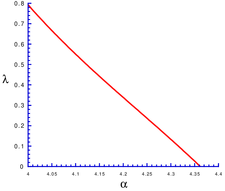
I have numerical studied the properties of for large (up to ) finding little dependence (as expected). I find that for for large :
| (22) |
where is positive for and vanishes at . For , but not too large both - and go to the same probability distribution, but does not go to zero. In other words is maximum Liapunov exponent: when it is negative the iteration converges to a fixed point, while when it is positive chaos is present.
The estimated value of , i.e. 4.36, is larger that the value where the complexity vanishes (i.e. 4.27), so that the previous conjectures should be correct in the interesting region of positive complexity, where there should be solutions of the satisfiability conditions that correspond to the solutions of the survey propagation equations.
The reader should notice that the survey propagation equations do have a solution also for and the fact that the complexity turns out be negative is a warning that original satisfiability problem does not have any solution. In this case the heuristic construction of the surveys is empty.
4 Conclusions.
The main propose of this note is the construction (following Aldous [18]) of the infinite rooted tree associated to given satisfiability problem. This infinite rooted tree plays the role of a bridge among a finite instance of the problems and the infinite random tree where analytic computations [1, 2, 12, 13] are done. It is argued that existence of an unique stable solution on the infinite tree (that apparently holds for ) implies the existence of an unique stable solution of the survey equations on a large system in the same range of .
This result implies that the survey equations that have been used [1, 2] in an algorithm to find an actual solution of an instance of the K-sat problem do have a solution. However independently from the interest of this application of the survey equations, I believe that the conjectures that have been put forward have a mathematical interest in their own because they clarify the fundamental hypothesis behind the approach of [1, 2, 12, 13]; eventually they can be used to prove similar results in other problems (like the -spin model).
Acknowledgements
I thank Marc Mézard and Riccardo Zecchina for useful discussions and encouragement.
References
- [1] M. Mézard, G. Parisi and R. Zecchina, Science 2002 in press.; Sciencexpress 27 June 2002.
- [2] M. Mézard and R. Zecchina The random K-satisfiability problem: from an analytic solution to an efficient algorithm cond-mat 0207194.
- [3] S.A. Cook, D.G. Mitchell, Finding Hard Instances of the Satisfiability Problem: A Survey, In: Satisfiability Problem: Theory and Applications. Du, Gu and Pardalos (Eds). DIMACS Series in Discrete Mathematics and Theoretical Computer Science, Volume 35, (1997)
- [4] S. Kirkpatrick, B. Selman, Critical Behaviour in the satisfiability of random Boolean expressions, Science 264, 1297 (1994)
- [5] Biroli, G., Monasson, R. and Weigt, M. A Variational description of the ground state structure in random satisfiability problems, Euro. Phys. J. B 14 551 (2000),
- [6] Dubois O. Monasson R., Selman B. and Zecchina R. (Eds.), Phase Transitions in Combinatorial Problems, Theoret. Comp. Sci. 265, (2001);
- [7] J.S. Yedidia, W.T. Freeman and Y. Weiss, Generalized Belief Propagation, in Advances in Neural Information Processing Systems 13 eds. T.K. Leen, T.G. Dietterich, and V. Tresp, MIT Press 2001, pp. 689-695.
- [8] Mézard, M., Parisi, G. and Virasoro, M.A. Spin Glass Theory and Beyond, World Scientific, Singapore, 1987.
- [9] F.R. Kschischang, B.J. Frey, H.-A. Loeliger, Factor Graphs and the Sum-Product Algorithm, IEEE Trans. Infor. Theory 47, 498 (2002).
- [10] Monasson, R. and Zecchina, R. Entropy of the K-satisfiability problem, Phys. Rev. Lett. 76 3881–3885(1996).
- [11] C. De Dominicis and Y. Y. Goldschmidt: ‘Replica symmetry breaking in finite connectivity systems: a large connectivity expansion at finite and zero temperature, J. Phys. A (Math. Gen.) 22, L775 (1989).
- [12] M. Mézard and G. Parisi: Eur.Phys. J. B 20 (2001) 217;
- [13] M. Mézard and G. Parisi: ‘The cavity method at zero temperature’, cond-mat/0207121 (2002).
- [14] D.J. Thouless, P.A. Anderson and R. G. Palmer, Solution of a ‘solvable’ model, Phil. Mag. 35, 593 (1977)
- [15] O. Dubois, Y. Boufkhad, J. Mandler, Typical random 3-SAT formulae and the satisfiability threshold, in Proc. 11th ACM-SIAM Symp. on Discrete Algorithms, 124 (San Francisco, CA, 2000).
- [16] S. Franz and M. Leone, Replica bounds for optimization problems and diluted spin systems, cond-mat/0208280.
- [17] M. Talagrand, Rigorous low temperature results for the p-spin mean field spin glass model, Prob. Theory and Related Fields 117, 303–360 (2000).
- [18] D. Aldous, The zeta(2) Limit in the Random Assignment Problem, Random Structures and Algorithms 18 (2001) 381-418.